

Abstract
Knowledge of the number of causative loci is necessary to estimate the power of mapping studies of complex diseases. In the present article, we reexamine a theory developed by Risch and its implications for estimating the number L of causative loci affecting a complex inherited disease. We first show that methods based on Risch’s analysis can produce estimates of L that are inconsistent with the observed population prevalence of the disease. We demonstrate this point by showing that the maximum-likelihood estimate for L produced by the method of Farrall and Holder for cleft lip/cleft palate data is not consistent with the prevalence under the multiplicative model. We show how to incorporate disease prevalence and develop a maximum-likelihood method for estimating L that uses the entire distribution of numbers of affected individuals in families containing an affected individual. This method avoids the potential inconsistencies of the Risch method and has greater precision. We apply our method to data on cleft lip/cleft palate and schizophrenia.
Introduction
It has become apparent that positional cloning for complex diseases is more difficult than has previously been envisioned. Recently, Altmüller et al. (2001) conducted a comprehensive review of 101 whole-genome–scan studies of complex disease and found that only one-third of these produced significant linkages. Furthermore, few of the linkages that were significant were reproduced in other studies. The reasons for this lack of success are not clear. It is known that the power to detect linkage decreases as the number of loci affecting a disease increases, because the effect of each locus is lower on average. Therefore, having reliable estimates of the numbers of loci that affect complex diseases will help with the design of mapping studies.
At present, only one class of methods, based on the theory introduced by Risch (1990a), is available to estimate the number of loci, L, when genotype data for affected individuals are unavailable. In the present article, we will reexamine Risch’s theory and related theories, with the goal of developing a method for providing more-accurate estimates of the number of causative loci than are currently available. In doing so, we will show that Risch’s theory may be inconsistent with the data to which it is applied, meaning that, for some models, no combination of parameter values can account for observed prevalences and relative risks. We show a method that avoids this inconsistency and has greater precision than previous methods based on Risch's theory.
Risch (1990a) modeled a disease affected by loci that act either multiplicatively or additively, and he derived relationships between the relative risk of a disease in relatives with different degrees of relatedness (“λR” in his notation) as a function of the number of causative loci. He then used his theory to explore the dependence of relative risk on the number of causative loci, L. In two companion articles (Risch 1990b, 1990c), he examined the power to detect linkage in affected pairs of relatives under the additive and multiplicative models. Risch showed that the power to detect linkage to a locus depends on the relative risk attributable to that locus and that the power deteriorates quickly as L increases. Farrall and Holder (1992) extended Risch’s (1990a) theory and developed a maximum-likelihood method for the estimation of L under the multiplicative model. Farrall and Holder (1992) applied their method to data from a study of cleft lip/cleft palate (CLCP) and found that the 1-LOD support interval for the number of loci was very broad: 2→∞.
In the present article, we will first reexamine the relationship between the number of loci affecting a complex disease, the population frequency of the disease, and the relative risks, and we will show that estimates of the number of loci in a multiplicative model obtained from relative risks may be inconsistent with the observed prevalence of a disease. We will then introduce a new method for estimating the number of loci that avoids these inconsistencies and that, in two examples, gives more-precise estimates of the number of causative loci. We call this method—a form of complex segregation analysis—a “multiplex method,” because it is based on the entire distribution of numbers of affected individuals in families containing an affected individual. Our analysis is similar to that of Smith (1971), who derived recurrence risk formulas for groups of sibs and compared fits of single-locus and multifactorial threshold models. We extend Smith’s recurrence risk formulas to allow for multiplicative interactions among loci and to permit analysis of other groups of relatives. We then develop a maximum-likelihood estimator for the number of disease loci. We illustrate the use of our method by applying it to CLCP data previously analyzed by Farrall and Holder (1992) and schizophrenia data published by Hovatta et al. (1997).
The Risch Method
First, we will review Risch’s (1990a) theory. Take X and XR as indicator variables denoting the affected status of the proband and a type R relative. Then, the probability P(XR=1|X=1) is given by
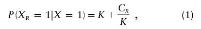 |
where K is the population prevalence of the disease and CR is the genetic covariance between type R relatives. Rearranging equation (1), we get
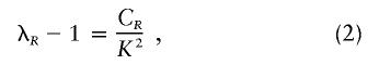 |
where λR, the “relative risk,” is given by P(XR=1|X=1)/K. The relative risks for two different types of relatives R and T are given by
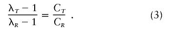 |
The above relationships apply for a single locus. Under a multiplicative penetrance model with no gametic disequilibrium, the overall relative risk is given by the product of the individual locus risks:
Assuming that equation (3) holds for each locus and substituting into equation (4), we get
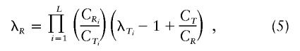 |
where L is the number of loci and C1, C2, and C3 are the locus-specific covariances for first-, second-, and third-degree relatives, respectively. Throughout the present article, the phrase “relative risk” refers to the total relative risk unless specified as “single-locus relative risk.”
Under the assumption that dominance variance is negligible, the relationship C1=2C2=4C3 holds, and equation (5) has a particularly simple form:
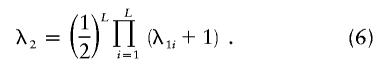 |
Risch (1990a) used equations (4) and (6) to compare different models of inheritance for schizophrenia. Risch also considered additive and genetic heterogeneity models. He showed that the genetic heterogeneity model is well approximated by the additive model and that the additive model gives the same pattern of relative risk as a single-locus model does. Risch (1990a) noted that, in many cases, relative risk decreases more rapidly with relatedness than is predicted by the additive model but that the multiplicative model can be parameterized to provide an approximate fit to observations. We will employ the multiplicative model here because of its mathematical simplicity and because, in the absence of other knowledge, it is reasonable. It remains to be established how realistic the multiplicative model is or what its relationship is to more-general models of epistatic interactions.
Risch (1990a) employed an informal approach for the comparison of inheritance models. Farrall and Holder (1992) introduced a method using equation (6) as the basis for a maximum-likelihood method for the estimation of L under the assumption of equal contribution to disease risk by all loci. We will refer to these methods jointly as the “Risch-Farrall-Holder” (RFH) method, and we will refer to the maximum-likelihood method as the “Farrall-Holder” (FH) method. In both cases, we are referring to the method for the inference of parameters of a model of inheritance, as opposed to the relationships given by equations (1)–(6).
Inconsistency of RFH Method with Observed Population Prevalences
We will now show that the best-fit (either formal or informal) models given by the RFH method are often inconsistent with the observed population prevalence of the disease. Several authors (Suarez et al. 1976; Craddock et al. 1995; Rybicki and Elston 2000) have explored the mathematical limits on the range of possible relative-risk values under different genetic models. Craddock et al. (1995) have described a graphical method for the determination of plausible modes of inheritance for complex traits and have applied it to bipolar disorder; they showed that the lower limit on possible sib-relative-risk values λS for bipolar disorder is not consistent with a single-locus model or any genetic heterogeneity model but that multiplicative models with three or more loci are plausible. Recently, Rybicki and Elston (2000) have studied the relationship between sib relative risk and genotype relative risk for one- and two-locus models; they looked at upper bounds on sib relative risk and showed that it is restricted to values <10 for many genetic models unless there is significant dominance. The results of these studies show that there are strong restrictions on the range of possible λS values.
Risch’s equations give information only about the values of λ2 and the values of λ3 relative to λ1. Thus, λ1 is treated as an independent parameter. However, we note that λ1 is itself dependent on L. Thus, the use of equation (5) implicitly assumes that, for every L, there is some combination of penetrance values and disease-allele frequencies that gives λ1. We now show that this is not always true.
We will assume that all disease-predisposing alleles at a locus have equal affect. Thus, we must track only two allele types: disease-causing and non–disease-causing alleles (hereafter referred to as “disease alleles” and “nondisease alleles,” respectively). Although this is less general than in Risch's (1990a) study, this case is of sufficient importance to illustrate the point. Take π as the probability that the lowest-penetrance genotype (individuals homozygous for the nondisease allele on every locus) is affected and δ as the probability that the highest-penetrance genotype (individuals homozygous for the disease alleles on every locus) is affected. If we assume equal contribution to disease penetrance by all loci, then the single-locus contributions to π are πL=π1/L, and the single-locus contributions to δ are δL=δ1/L. If we introduce a dominance coefficient h, then the three single-locus penetrance contributions are given by πL, πL+h(δL-πL), and δL, for nondisease-allele homozygotes, heterozygotes, and disease-allele homozygotes, respectively.
The genetic model is completely specified by a choice of L, h, π, δ, and disease-allele frequency p. Thus, as L is varied in the application of the RFH method, it is (implicitly) assumed that there exist values of π, δ, h, and p that will yield λ1. If dominance variance is negligible, then parent-offspring and sib genetic covariances are equal. In this case, the parent-offspring and sib relative risks are also equal. Because this is observed for most complex diseases, it is usually assumed that there is no dominance variance, and, thus, h is restricted to regions where this is approximately true. We will use this assumption and constrain parameter values in the following analysis (but not in the application of our method in the “Multiplex Relative Risk” section, below).
In appendix A, we derive equations for the probability that a disease affects an individual given that some collection of relatives is affected. We can use this procedure to find the joint probability that parent and offspring are both affected:
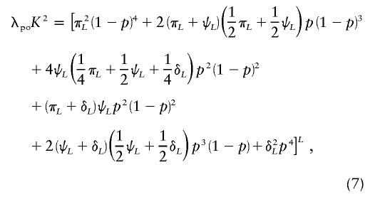 |
where 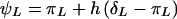 , p is the disease-allele frequency, and λpo is the parent-offspring relative risk. This equation gives parent-offspring risk directly, in terms of the genetic model, and is therefore fully consistent with all parameters. In addition to satisfying equation (7), the set of parameters must also produce the correct disease prevalence K, given by
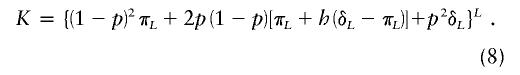 |
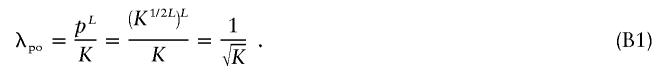
Furthermore, these parameters must satisfy 0<p<1, 0⩽π⩽K, and K⩽δ⩽1. Our goal is to find the maximum value of λpo given equations (7) and (8) and these constraints. We solve equation (8) for p and substitute into equation (7). This gives an expression for λpo that is constrained to allow the observed disease prevalence K. The prevalence is assumed to be known exactly. Given the large sample sizes typical for prevalence, this should usually be reasonable. The dependence that this expression has on the parameters is complex and is further complicated by the somewhat vague requirement that dominance variance be negligible. In appendix B, we derive expressions for the maximum λpo value for h=0, h=1/2, and h=1, and we show that, when the dominance coefficient is unrestricted, λpo is always maximized at either h=0 or h=1. For large values of L, the dominance variance is negligible regardless of h, and the maximum λpo value is given by  . In this case, λpo has a maximum value of 10 for L⩾10 and K=0.01 and a maximum value of 36.6 for L⩾10 and K=0.001.
For small-to-intermediate values of L, the dominance variance is not negligible for all values of h. In this case, we have resorted to numerical explorations of the parameter space, to find maximum possible values of λpo. Table 1 shows the maximum values of λpo and λS (sib relative risk) for K=0.01 and K=0.0001 and various values of L for when the dominance coefficient is restricted such that λS⩽1.11×λpo. Under the requirement λS⩽1.11×λpo, the maximum possible value of λpo is 7.8 for L=5–10 and K=0.01 and is 11.6 for L=10 and K=0.001. It is debatable whether we should consider that λS>1.11×λpo indicates nonnegligible dominance variance, but, regardless of the exact condition that we use, it is clear that there are strong restrictions on possible values of λpo. Thus, for example, schizophrenia and bipolar disorder, which both have a prevalence of 0.01 and have first-degree relative risks of ∼10 (Risch 1990a) and ∼15, respectively (Altmüller et al. 2001), are strongly restricted in possible models. In particular, it is difficult to produce large relative-risk values with intermediate numbers (∼5–12) of loci. Larger relative-risk values can be produced for models with many loci (>15) but only under restrictive parameter assumptions (typically, h=0, πL=0, and δL=1).
Table 1.
Maximum Relative Risk[Note]
| K | L | Maximum λpoa | Maximum λSa | hb |
| .001 | 5 | 54.8 | 60.0 | 1 |
| .001 | 10 | 11.6 | 12.5 | .3 |
| .001 | 15 | 15.4 | 17 | .2 |
| .001 | 20 | 18.7 | 20.7 | .1 |
| .001 | 50 | 31.6 | 33.6 | 0 |
| .01 | 5 | 7.8 | 8.4 | .8 |
| .01 | 10 | 7.8 | 8.6 | .1 |
| .01 | 15 | 10.0 | 10.9 | 0 |
| .01 | 20 | 10.0 | 10.7 | 0 |
| .01 | 50 | 10.0 | 10.3 | 0 |
Note.— The values of πL and δL were 0 and 1, respectively, for all cases except δL=.7 for K=.001 and L=20.
Greatest allowable values of λpo and λS under the restriction of λS⩽1.11×λpo (i.e., small dominance variance) as a function of number of disease loci L and disease prevalence K.
Value of h for the maximum values of λpo and λS.
When h is restricted to 0.5 (no dominance), we can get a simple formula (eq. [B7]) for the allowable values of λpo. Figure 1 shows a plot of allowable values of λpo as a function of L for K=0.01 and K=0.001. Points below the curves are allowable combinations of L and λ1. In this case, the limits on allowable values of λpo are very stringent. For example, schizophrenia could not involve more than two loci in this case. As L increases, the disease-allele frequency also increases, and it takes substantial dominance to get large relative-risk values.
Figure 1.

Allowed values of sib relative risk λS. The curves correspond to the overall disease prevalence K, as shown. Only combinations of λS and L under the curve are possible. The curve is given by equation (B7) and is valid only for the case of no dominance (h=1/2).
The reason that the range of values of relative risk is restricted is that the prevalence K determines the disease-allele frequency for a given set of parameters. In the absence of this constraint, the relative risk simply increases with L—the more loci that are necessary for the disease, then the more important potential identity-by-descent (IBD) sharing with an affected relative is for the occurrence of the disease. However, if the prevalence is accounted for, L cannot be increased without an increase in p. Figure 2a shows plots of p versus L, obtained by solving equation (8) for p. We see that p increases rapidly with L. If L increases, then the number of “disease events” that must occur for an individual to be affected also increases. Thus, the probability of a disease event must increase to keep K constant. The relative risk, in turn, has a strong dependence on p. Figure 2b shows plots of sib relative risk versus L for values of πL ranging from 0 to 0.2 (with h=0.5 and δL=1). As expected, the highest relative risks occur for πL=0. At πL=0, the relative risk decreases from 10 to 4, between L=1 and L=10, as p increases from near 0 to near 0.6. The relationship is more complicated for πL>0 (meaning that some single-locus disease events occur without disease genotypes). Then, the disease-allele frequency increases less rapidly with L, because it is possible for some of the L required disease events to occur without any disease alleles. Increasing L has two opposing effects on the relative risk: the number of required disease events increases (tending to increase relative risk), but the probability of those disease events also increases (tending to decrease relative risk). The value of πL determines which effect dominates; thus, it is possible for relative risk to either increase or decrease with L (see fig. 2b). Note, from figure 2b, that the maximum possible sib relative risk always decreases with L.
Figure 2.

Effect of varying L. a, Effect of number of loci L on disease-allele frequency p. The curves correspond to values of the dominance coefficient h, as shown, and to K=0.01, δL=1, and πL=0.2. b, Effect of L on sib relative risk. The curves were generated with πL values of 0, 0.02, 0.05, 0.1, 0.15, and 0.2, ordered from top to bottom, as shown. For all plots, δL=1, and h=0.5.
The shape of the curves in figure 2 is strongly dependent on the assumption of multiplicative interactions between loci. Under an additive model, for example, the disease-allele frequency decreases linearly with increasing number of disease loci. The sib relative risk increases with L for small values of πL and decreases with L for larger values of πL—a pattern opposite to that for the multiplicative model.
We should stress that table 1 and figure 1 are valid only for loci of equal effect under a multiplicative model. Obviously, there are more ways to satisfy the parameter constraints when the loci can vary independently. However, the general patterns still hold. For example, a popular model for genetic epidemiological studies assumes one or a few major genes and many minor genes. A simple extension of the methods used in the present article for a disease with K=0.01 shows that such a model is possible only for multiplicatively interacting loci if (i) the major gene (or genes) has h near 0.5, (ii) there are ⩾20 of the minor genes, and (iii) the minor genes have parameters very near h=0, πL=0, and δL=1.
Environmental Correlations and Ascertainment Bias
Relative-risk values are a measure not only of genetic similarity but also of environmental similarity (Guo 2000, 2002). Thus, the observed values will often be inflated beyond the genetic-effect–only values assumed in Risch’s (and our) method. The presence of environmental correlation will cause the estimate for L to be biased downward. Even with no environmental correlations, relative-risk estimates are subject to ascertainment bias (Rice et al. 1982; Guo 1998; Cordell and Olson 2000; Olson and Cordell 2000). Such bias can occur for a variety of reasons, including a greater probability of the detection of families with more affected members, variations in the probability that affected individuals have children, reluctance of parents of an affected individual to have further children, and an increased probability that relatives of an affected individual are falsely diagnosed as affected. Although there are definite problems with data on recurrence risk even for first-degree relatives, the need to use data on second- and third-degree relatives in the RFH method magnifies the problem. An important advantage of our method is that it does not require data from multiple types of relatives. Thus, relatives with known or suspected bias in affected probabilities can be eliminated from the analysis. We will show, in our examples, that estimates from our method are fairly robust to variations in which relative types are included in the analysis.
Multiplex Relative Risk
We estimate L by using a maximum-likelihood approach. The likelihood function F is a product of multinomial distributions for the number of affected relatives of probands:
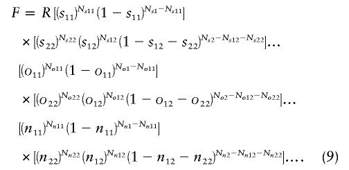 |
In equation (9), sij is the probability that i of j sibs of the proband are affected; Nsj is the number of probands with j sibs; Nsij is the number of probands with i of j sibs affected, and so forth; and oij and nij refer to offspring and nieces/nephews, respectively. This can be extended to any type of relative. The probabilities sij, oij, etc., are functions of L, h, δL, and πL. The derivation for the probabilities for sibs is given in appendix A. The probabilities for other types of relatives are calculated in a similar fashion. The quantities Nsj, Nsij, and so forth, are the input data. R is an arbitrary constant.
The likelihood is maximized over the range of values of L = [1–100], h = [0–1], π = [0–K], and δ = [K–1], for the data Nsj, Nsij, and so forth, and the prevalence K. The frequency p of the disease allele is calculated from the prevalence and the assumed genetic model for the disease. Note that the dominance coefficient is not restricted for these model fits. The support interval is taken as all sets of L, h, πL, and δL that are not less than one-tenth as likely as the maximum-likelihood value.
Precision of Methods
Figure 3 shows a plot of equation (5) for λS=10 (the first-degree relative risk for schizophrenia), CR/CS = 1/2, and varying L. With this choice of parameters, λR corresponds to the relative risk for second-degree relatives (e.g., aunt and nephew). Most of the change in λR occurs between L=1 and L=3, and very little change occurs beyond L=5. Thus, this relationship gives us a weak basis for making inferences about L outside this range. However, this relationship does give us a basis for distinguishing between single-locus and multilocus models and can reliably set the lower bound on L as single locus or multilocus.
Figure 3.

Aunt-nephew relative risk as a function of L for a parent-offspring relative risk of 10. This curve was generated by equation (5) with λR=10 and CR/CS=1/2.
The RFH method bases inference on equation (5). Only the ratios of relative-risk values are used. Figure 2b shows that the risk for first-degree relatives itself provides substantial information about L. However, for smaller L (e.g., L<10), there is a wide range of possible values of the relative risk as πL is varied. When h (especially) and δL are also varied, the range is further increased. Thus, if all of these parameters are free when the model is fitted to data, then it will be difficult to use λpo to distinguish among values of L in this range. As discussed earlier in the present article (see the “Inconsistency of RFH Method with Observed Population Prevalences” subsection), there are strong restrictions on the maximum possible value of λpo. Thus, constraining the values of λpo when fitting data can provide an upper bound on the interval of plausible values of L.
In view of these arguments, we would expect that, if fits to a model are based on simple relative-risk values by using equations (5) and (7), only loose upper and lower bounds on L would be obtained. The distribution of numbers of affected sibs provides additional information. For example, figure 4 shows the probability that two of three and three of three sibs of a proband are affected when L is in the range of 3–10. Their absolute and relative values vary substantially over this range. Estimates of these multiplex probabilities for families of various sizes provide additional information about the range of L values that is most important. However, we also see, from these figures, that the probabilities of having two or more affected sibs are quite small. The probabilities in figure 4 are conditioned on the proband's being affected. We multiply by the prevalence (0.01 in the case of fig. 4) to get the marginal probabilities. Thus, sample sizes will need to be large to have enough such families to appreciably affect the likelihood functions.
Figure 4.

Effect of number of disease loci on multiplex-disease probabilities. a, Probability that two of three sibs of an affected individual are also affected. b, Probability that three of three sibs of an affected individual are also affected. Both curves were generated with K=0.01, h=0.5, δL=1, and πL=0.
Applications to Data
CLCP
We apply our method to one of the data sets used by Farrall and Holder (1992). Farrall and Holder (1992) used equation (5) as a basis for a maximum-likelihood approach to estimating L for CLCP. We will reanalyze the data of Carter et al. (1982), which provide sufficient information to estimate the multiplex probabilities. Farrall and Holder (1992) combined data from the Carter et al. study with data from other studies from which multiplex probabilities cannot be estimated. We recompiled the data given by Carter et al. (1982) to get the probabilities that 0, 1, 2, and so forth, relatives of a proband with CLCP were affected (data for first-degree relatives are given in tables 2 and 3; similar tables for second-degree relatives are available at Paul Schliekelman’s Web site).
Table 2.
CLCP Data and Best-Fit Model from Multiplex Method—Offspring
|
No. of Familiesc with |
|||||||
| No Individuals Affected |
One Individual Affected |
Two Individuals Affected |
|||||
| No. of Childrena | Overall No.of Familiesb | Observed | Expected | Observed | Expected | Observed | Expected |
| 1 | 86 | 83 | 83.7 | 3 | 2.3 | … | … |
| 2 | 183 | 170 | 173.8 | 13 | 8.7 | 0 | .5 |
| 3 | 97 | 90 | 90.0 | 7 | 6.2 | 0 | .7 |
| 4 | 34 | 32 | 30.9 | 2 | 2.6 | 0 | .4 |
| 5 | 13 | 12 | 11.6 | 0 | 1.1 | 1 | .2 |
| 6 | 8 | 5 | 7.0 | 3 | .8 | 0 | .2 |
| 8 | 2 | 1 | 1.70 | 1 | .2 | 0 | .07 |
| 9 | 1 | 0 | .84 | 1 | .1 | 0 | .04 |
Number of offspring of the proband.
Number of families with the given number of offspring.
Observed and expected numbers of such families with zero, one, or two affected children of affected individuals; no family had more than two individuals affected. Observed values were compiled from Carter et al. (1982); expected values were calculated from the best-fit model of L=3, h=.9, δL=1, and πL=.05.
Table 3.
CLCP Data and Best-Fit Model from Multiplex Method—Sibs
|
No. of Familiesc with |
|||||||||
| No Individuals Affected |
One Individual Affected |
Two Individuals Affected |
Three Individuals Affected |
||||||
| No. of Sibsa | Overall No.of Familiesb | Observed | Expected | Observed | Expected | Observed | Expected | Observed | Expected |
| 1 | 122 | 118 | 118.7 | 4 | 3.3 | … | … | … | … |
| 2 | 80 | 77 | 75.9 | 3 | 3.8 | 0 | .2 | … | … |
| 3 | 62 | 57 | 57.5 | 4 | 4.0 | 0 | .5 | 1 | .03 |
| 4 | 41 | 39 | 37.2 | 2 | 3.2 | 0 | .5 | 0 | .06 |
| 5 | 17 | 16 | 15.1 | 1 | 1.5 | 0 | .3 | 0 | .05 |
| 6 | 18 | 17 | 15.7 | 0 | 1.7 | 1 | .4 | 0 | .09 |
| 7 | 8 | 7 | 6.9 | 0 | .8 | 1 | .2 | 0 | .06 |
| 8 | 5 | 4 | 4.2 | 0 | .5 | 1 | .2 | 0 | .05 |
| 9 | 7 | 6 | 5.8 | 1 | .8 | 0 | .3 | 0 | .09 |
| 10 | 3 | 3 | 2.5 | 0 | .3 | 0 | .1 | 0 | .05 |
| 11 | 2 | 2 | 1.6 | 0 | .2 | 0 | .1 | 0 | .04 |
| 13 | 1 | 1 | .79 | 0 | .1 | 0 | .05 | 0 | .02 |
Number of sibs of the proband.
Number of families with the given number of sibs.
Observed and expected numbers of such families with zero, one, two, or three affected sibs of affected individuals; no family had more than three individuals affected. Observed values were compiled from Carter et al. (1982); expected values were calculated from the best-fit model of L=3, h=.9, δL=1, and πL=.05.
Using the FH method on the Carter et al. data (1982), we find a maximum-likelihood estimate of L=22 with a support interval of 4→∞. Table 4 shows the observed relative-risk values along with those for the best-fit model. The observed parent-offspring and full-sib relative risk values were 32.1 and 28.5, respectively. The maximum possible (unrestricted dominance) value for λpo is 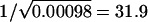 , occurring if the disease allele is completely recessive and the disease is completely genetically determined (i.e., if πL=0 and δL=1). The corresponding λS of 36.6 is not compatible with the observed value. If we restrict the dominance and ensure that λS⩽1.11×λpo, then the maximum value of λpo (obtained numerically) is 22.1 (occurring at h=0.1, πL=0, and δL=1). Thus, the best-fit value from the FH method does not appear to be compatible with the observed disease prevalence. Note that the allowance of even small deviations from complete penetrance causes the maximum value of λpo to decrease substantially. For example, the maximum value of λpo is 23.6 if we take δL=0.97 in the unrestricted dominance case. The maximum value of λpo drops to 16.9 for δL=0.97 in the restricted dominance case. Similar reductions in maximum value of λpo occur if we allow πL to differ from 0. If we specify no dominance (in view of the observation that λS<λpo in the data), then the highly restrictive limits on λpo shown in figure 1 apply and none of the best-fit models given by Farrall and Holder (1992) are compatible with the observed prevalence.
Table 4.
Fits of CLCP Data[Note]
| K | λ1 | λ2 | λ3 | |
| English dataa | .98/1,000 | 30.3 (2,053) | 5.7 (5,139) | 2.8 (4,744) |
| MLE modelb (L=22) | .98/1,000 | 29.6 | 5.8 | 2.5 |
Note.— Results from the FH method (Farrall and Holder 1992).
Relative-risk data from an English study of CLCP (Bear 1976; Carter et al. 1982). Following the procedure of Farrall and Holder (1992), we assumed that there was no dominance variance and combined all relatives of the same degree together. Numbers in parentheses are sample sizes.
Relative-risk values calculated for the best-fit model of 22 loci with equal contribution to disease risk. MLE = maximum-likelihood estimate.
Figure 5a shows the likelihood profile for L obtained using multiplex relative risk. In all likelihood plots, the likelihood value shown is the maximum across all parameters not shown. We see a strong peak in the likelihood in the range of L=3–6, with the likelihood dropping off quickly both as L decreases to 1 and as L increases beyond 10. The likelihood then begins increasing again beyond 14 and continues increasing as L goes to 100 and beyond. Figure 5b shows a contour plot of likelihood versus L and h and helps to clarify these peaks. The contours show combinations of L and h with likelihoods 1/2, 1/10, and 1/100 of the maximum-likelihood values. We see that there are two distinct peaks in the likelihood, one at L=3 with h being higher (but a range of 0.2–1 falling in the 1-LOD support interval) and one at L⩾100 with h being restricted to values around 0. A model with ⩾100 disease loci does not seem plausible, so this higher peak appears to be an artifact. If we dismiss it from consideration, then we find that our best-fit–value model has L=3, h=0.9, δL=1, and πL=0.05. The support interval for L is 2–14. There is a second peak, at L=6, that is only slightly below the L=3 peak. Figure 6 shows contour plots for L and δL (fig. 6a) and L and πL (fig. 6b). The fits of L are quite robust to variation in δL and πL. The 1-LOD support space encompasses a wide range of values of both parameters, with the range of values of L becoming broader as πL goes to 0 and δL goes to 1.
Figure 5.

Likelihood profiles for CLCP data. a, Likelihood profile for L. b, Contour plot of the likelihood versus L and h. The likelihood value shown is the maximum across the parameters not shown. The values shown on the contour lines are the likelihood of parameter combinations on that contour relative to the maximum-likelihood value. The likelihood for the multiplex-relative-risk method was generated using equation (9) and data from Carter et al. (1982) on offspring and sibs of probands. The log(0.1) curve shows the cutoff for the support interval (which includes all L values that are at least one-tenth as likely).
Figure 6.

Likelihood contours for CLCP data. a, Likelihood of the CLCP data versus L and δL. b, Likelihood versus L and πL. For each L, δL ranged from slightly above K1/L (the lowest possible value) to 1, in increments of 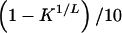 . The Y-axis units gives these increments. Thus, the value of the Y-axis units in panel a changes with the X-axis variable L. The same holds for panel b: πL ranged from 0 to K1/L in increments of K1/L/10, and the Y-axis units have the same value.
As we have shown, the possible relative-risk values depend strongly on L. Including the actual values of the risk (as opposed to just the relative values between different degrees of relatedness) substantially increases the sensitivity of the likelihood function to L and is the major cause of the increase in precision. The number of families with more than two affected individuals is quite small for the CLCP sample sizes. The exclusion of such data from the analysis had only a minor effect on the likelihood function. The addition of first cousins also had very little effect on the likelihood profile, other than shifting the maximum-likelihood–estimate value from the L=3 to the L=6 value.
Tables 2 and 3 show the numbers of affected first-degree relatives predicted by the best-fit model from the multiplex method, along with the observed values. The predicted values fit the data well. However, there does appear to be a slightly higher incidence of families with more than one relative of the proband affected. Similar tables for second-degree relatives are available at Paul Schliekelman’s Web site.
Application to Finnish Schizophrenia Data
To further demonstrate the utility of our method, we will also apply it to schizophrenia data. Hovatta et al. (1997) identified all cases in Finland with a diagnosis of schizophrenia and published the number of affected sibs in families (nearly 20,000) with up to 15 sibs (the data set used in our analysis is available at Paul Schliekelman’s Web site). We applied the multiplex method to these data. The best-fit value was L=3 with a support interval of [2,3], and h=1, δL=1, and πL=0.04.
Hovatta et al. (1999) conducted a genomewide scan for schizophrenia genes in a genetic isolate of Finland and found evidence for linkage at four loci. Thus, our results for the entire Finnish population are roughly compatible with this finding.
For this data set, we get a very tight support interval for L. Because there are substantial numbers of families with more than one relative affected, the use of multiplex data in our fitting procedure makes a substantial difference in precision. Results were essentially the same when families with more than four sibs were excluded from the data. However, the exclusion of smaller family sizes resulted in different best-fit values and a major loss of precision (i.e., support intervals of 2→∞ for L).
We also see much tighter bounds on h, δL, and πL. The support region for h extended from 0 to 0.15. The support region for δL was limited to values near 1, whereas that for πL was limited to values in the middle of the range (corresponding to πL in the range 0.05–0.2).
Because there are no parent-offspring data in this data set, there is nothing that constrains sib and parent-offspring risks such that they are similar. The best-fit model does predict substantially different risks for parent-offspring pairs and sibs of probands, which is not consistent with other data on schizophrenia. We added 5,000 simulated parent-offspring pairs to the data, to test the importance of not having parent-offspring data. These pairs were assigned the same relative risk as observed for sib pairs in the data set. This is consistent with other data on schizophrenia (Risch 1990a). The best-fit model (see table 5) had significant changes only in the dominance coefficient h, which became 1. Thus, the model fits were robust to this lack of data. However, it is clear that some parent-offspring data are needed to get correct estimates of h.
Table 5.
Best-Fit Values for Schizophrenia Data[Note]
Note.— Maximum-likelihood values of model parameters for Finnish schizophrenia data.
Parameter fits with data from Hovatta et al. (1997).
Five thousand offspring parent-offspring pairs with relative risk equal to that for a single sib were added to the data. This was to force a realistic value of h.
The best-fit model for CLCP had L = 3 and πL = 0.05. Thus, a person with no disease alleles would have 0.053 = 0.000125 probability of being affected; this compares to 0.001 for a randomly chosen individual. For the best-fit schizophrenia model, the disease probability for an individual with no disease alleles is 0.154=0.0005; this compares to 0.01 for a randomly chosen individual. In contrast, both best-fit models had δL=1. This indicates no environmental variation in the contribution from a locus homozygous for the disease allele. In this case, an individual homozygous for the disease allele on all loci is always disease affected. Both disease models were quite robust to variation from δL=1.
Discussion
As shown by Risch (1990b), the power of mapping studies for complex traits is dependent on the number of causative loci. Altmüller et al. (2001) compared characteristics of various mapping studies in an attempt to determine which factors lead to occurrence of significant linkage; they found that sib relative risk was uncorrelated with detection of significant linkage, and they concluded that, contrary to the results of Risch (1990b), sib relative risk is not a strong indicator of power in these studies. However, Altmüller et al. (2001) neglected an important point: the power to detect significant linkage in a study of affected pairs of relatives depends not on the overall relative risk but on the relative risk attributable to each locus and on how the loci interact (Risch 1990b). Thus, we do not expect to see a strong correlation between the observed relative risk and the power.
Because of the importance of contributions from each locus, methods for estimating the number of causative loci will be important for the design of mapping studies (Risch 1990b, 1990c). We have shown here that caution must be used in the application of the methods of Risch (1990a) and Farrall and Holder (1992). Our analysis has shown that the application of these methods can give results that are inconsistent with the observed disease prevalence. The maximum possible parent-offspring relative risk decreases rapidly as the number of loci underlying the disease increases, and the RFH method does not constrain it to feasible values. The multiplex method introduced here is a generalization of the RFH method and is guaranteed to give consistent results.
We have also shown that the precision of inference of L on the basis of the RFH method is of major concern. Often, this method can say nothing more than that the number of causative loci is >1. The multiplex method has improved precision. For the CLCP example, which had sample sizes on the order of a few hundred families, our method yielded a support interval of [2,14], compared with [2,∞] for the RFH method. Although this is not as good as we might like, [2,14] is a much more useful bound than [2,∞]. Our method yielded a very precise (i.e., [2,3]) estimate with the much larger sample size (∼20,000 families) of the schizophrenia data. For higher (greater than ∼10) best-fit values of L, the precision of the method decreases. The support intervals in such cases generally extend to infinity on the upper end and a maximum of 10–15 on the lower end (P.S., unpublished data). This tendency is due to the phenomenon illustrated in figure 2: under a multiplicative model, the variation at individual loci becomes small as L becomes larger. Thus, there is little change in patterns of inheritance with greater numbers of loci. Although precision does decrease as the best-fit L increases, the multiplex method still has better performance than the RFH method: knowing that L is >10 is much more useful than knowing only that it is >2.
As pointed out by an anonymous reviewer, some disease loci are known for some complex diseases. Thus, what is unknown is how many disease loci remain, as opposed to the total number. If the relative-risk value attributable to a known locus can be determined, then it can be divided out of the overall relative risk under a multiplicative model. The method described here can then be applied to the remaining loci.
Ascertainment Bias and Environmental Correlation
Fits of L in the applications in the present article were robust to variations in which data were included in the analysis. This indicates that it is possible to perform the analysis on subsets of available data and thus exclude suspect data. In cases in which it is not possible to exclude all biased data, it may be possible to include only data biased in the same direction. For example, data that are biased toward higher relative risks will tend to produce lower estimates of L. In this case, one could still get a lower bound on L and an upper bound on power in mapping studies. The RFH method requires data from individuals of at least two different degrees of relatedness.
Penetrance Models and Power of Mapping Studies
For CLCP and schizophrenia, the best-fit models had three and four loci, respectively. On the basis of the power relationships in Risch's (1990b, 1990c) studies, affected-sib-pair studies for both these diseases should then have 80% power for sample sizes of ∼200 (assuming λS=30 for CLCP and λS=10 for schizophrenia and marker density such that the recombination fraction is ∼0 between marker and disease allele). For CLCP, the support interval for L extended up to 14. In this case, sample sizes of ⩾1,000 would be required in order to achieve reasonable power. It is unknown, however, how reasonable the assumption of equal contribution from all loci is. Under that assumption, the estimated value of L leads to a lower bound on the contribution from each locus. This then indicates what sample sizes and marker densities will be necessary to map causative loci (Risch 1990b, 1990c). From the point of view of mapping, assumption of equal effects is conservative. Variation among loci will ensure that at least one causative locus will have an effect greater than the lower bound. Recently, Pritchard (2001) modeled the evolution of complex-disease loci. He showed that, because of intrinsic variability in allele frequencies created by genetic drift, mutation, and, possibly, weak purifying selection, contributions of different loci would be expected to vary substantially because of variation across loci in the frequencies of causative alleles. On this basis, he argued that a higher number of loci is likely for complex diseases, since the evidence from affected-sib-pair studies is against any single locus's having a major effect. Although Pritchard’s (2001) analysis was based on specific population genetic assumptions, his conclusion that substantial variation of effects across loci is to be expected is almost certain to be correct for a much wider class of models than he considered.
It would be possible to incorporate variation across loci into our multiplex method. A statistical distribution (e.g., a gamma distribution) of effects could be assumed, or a population genetic model of the kind used by Pritchard (2001) could be analyzed. In either case, the resulting model might be so rich in parameters as to be impractical.
As with all model fitting, the information that we get is only as good as the model. It is completely unknown whether a multiplicative model is in any way representative of reality. It is the case that a multiplicative model can match the available risk data for CLCP and schizophrenia quite well. Using the methods outlined in the present article, we can gain much information about the implications if a multiplicative model is the correct description for a disease. However, there is no way of knowing whether a different model is more appropriate. Future work should extend the present methodology to more-general penetrance models. The primary obstacle to overcome is the large number of genotype probabilities that must be calculated when the assumption of multiplicative interactions does not apply. The popularity of multiplicative penetrance models is based on nothing more than mathematical convenience. Thus, it is important to move beyond such models. Although it is impossible to ever prove that a model is correct by using only family-history data, we can exclude models. One major success of the RFH method is showing that a model with additive action between loci is not plausible for either schizophrenia (Risch 1990a) or CLCP (Farrall and Holder 1992). Future work should test other penetrance models and decide on their plausibility and, if they are plausible, the implications thereof.
Acknowledgments
This research was supported in part by grant GM40282 (to M.S.) from the National Institutes of Health. We thank C. Garner for helpful discussions.
Appendix A: Derivation of Probabilities of Affected Status
Our goal is to derive equations that give the probability that M of N relatives of an affected individual are affected. We will demonstrate the derivation for two sibs of the affected individual. The derivation is similar for other types and numbers of relatives.
Take X, XS1, and XS2 as indicator variables representing the affected status of the proband and sibs 1 and 2, respectively. These indicator variables have a value of 0 when the individual is unaffected and a value of 1 when the individual is affected. Then,  is the probability that the sibs 1 and 2 are affected, given that the proband is affected.
We can expand this probability to include the parental genotypes:
where B1 and B2 represent the genotypes of the parents of the three sibs.
Using the Bayes theorem, we can rewrite the conditional probability of the parental genotypes as
 |
The genotype distributions of sibs are independent, given the parental genotype. Thus, the probabilities that sibs 1 and 2 are affected are independent, given the parental genotype. Hence, we have P(XS1=1,XS2=1|B1=b1,B2=b2) = P(XS1=1|B1=b1,B2=b2)P(XS2=1|B1=b1,B2=b2). Finally, the genotype distribution of the parents is also assumed to be independent. Then, equation (A1) becomes
 |
The probability of being affected given the parental genotype is the same for all children. Thus, we can write equation (A2) as
Equation (A3) can easily be extended to any number of sibs:
Next, we need the probability that an individual is affected given his or her parent’s genotypes. We expand this probability in terms of the individual’s genotype A, as follows:  =
=  .
.
Multiplicative Penetrance
To proceed, we need to further specify the penetrance model. Following Risch (1990a), we assume a multiplicative model for penetrance:  , where u(G) is the disease penetrance for multilocus genotype G and
  is the contribution to the penetrance from the one-locus genotype ij on locus j. Thus, G is a vector [i1,i2,…iL].
If there is no linkage disequilibrium, then the probability that n sibs of a proband are affected can be expressed as
 |
where jm and km index the parental genotypes. Equation (A4) can be rearranged as
Equation (A5) shows that the single-locus genotype frequencies can be calculated independently and then can be multiplied to get the overall probabilities.
Probabilities That Fewer Than All Sibs Are Affected
The probability that sib 1 is affected and sib 2 is unaffected is P(XS1=1,XS2=0|X=1)=P(XS2=0|X=1) − P(XS1=0,XS2=0|X=1). Thus,
This can be generalized as
 |
and so forth. Equations (A6)–(A8) are not specific to sibs and apply to any type (or combination of types) of relatives.
Appendix B: Derivation of Constraints on L
Our goal is to find, given L, the maximum parent-offspring relative risk that can be produced by an allowable combination of penetrance values and allele frequencies. This risk is given by the equation
 |
This is subject to the constraint that the parameters and allele frequencies must produce the correct disease prevalence K:
We have not found any general analytic proof on maximums for λpo. However, we can argue, on intuitive grounds, that it should be maximized at πL=0 and δL=1: the relative risk should be highest when disease risk is determined completely by genotype and has no environmental component. Numerical evidence supports this. If we assume that this is the case, then we can show that λpo will always be maximized at either h=0 or h=1 (the proof of this is straightforward, but algebraically intense and will not be shown here). We can easily find the maximums for λpo in these cases.
If the disease alleles are completely recessive (h=0), then an affected parent must be homozygous for the disease allele on all disease loci. Thus, it is certain that a child will receive a disease allele on each locus from that parent. We have not specified anything about the other parent. Therefore, the probability that this child receives a disease allele on a particular locus from that parent is simply the disease-allele frequency p. The probability that he or she receives the disease allele on all L loci is pL. The disease prevalence is given by K=p2L. Then,
 |
This gives λpo=10 for K=0.01 and λpo=31.6 for K=0.001. We can argue similarly to find the relative risk for sibs. Each parent of an affected person must be carrying at least one disease allele on each locus. At a particular locus, another child of those parents has a one-fourth chance of inheriting both of those alleles, a one-half chance of inheriting one of them, and a one-fourth chance of inheriting neither of them. In all cases, an allele that is not IBD with one that was inherited by the affected sib has the same frequency distribution as an allele selected from the general population. Thus, we have
For completely dominant disease alleles (h=1), the parent-offspring risk is given by
If the parent is a heterozygote—probability 2p(1-p)—then the child has a one-half chance of getting the disease allele on a given locus from that parent and has a (1/2)p chance of getting the normal allele from that parent and a disease allele from the other parent. If the parent is homozygous for the disease allele—probability p2—then the child always has a “disease event” for that locus. For completely dominant disease alleles, we have  . This can easily be solved for p and can be substituted into equation (B2). After doing this and comparing with equation (B1), we find that λpo is higher for h=0 than for h=1, when L⩾7 for K=0.01 and when L⩾10 for K=0.001. For large values of L, the sib and parent-offspring relative risks are nearly equal, even for completely recessive disease alleles. This is because the disease-allele frequency p increases as the power of 1/L and thus gets large very quickly with L (see fig. 2). When p is large, the probability of being homozygous for the disease allele at a given locus is large for everyone in the population, and sharing disease alleles IBD with a sib does not make much difference. For large values of L (such that the difference between λpo and λS is negligible), the maximum allowable λpo value will be given by equation (B1). For small-to-intermediate values of L, the dominance variance will be nonnegligible for h=0 and h=1. If the data indicate little or no dominance variance, then we must resort to a numerical approach to find the maximum allowable λpo value (see the main text).
We can also analytically solve the case with h=1/2 and general πL and δL. We start with equation (A5) and n=1 (note that λpo=λS for h=1/2):
 |
The disease prevalence is given by
If we take h=1/2 and simultaneously solve equations (B3) and (B4) for πL and δL, then we get
 |
and
 |
There are other solutions to equations (B5) and (B6) with the signs of the second terms reversed, but it can be shown that these solutions give values that are not bound between 0 and 1, as required for a probability. If we apply the restrictions 0⩽p⩽1 and 0⩽πL<K1/L<δL⩽1, then we can get the condition
 |
Craddock et al. (1995) obtained the condition (eq. [B7]) with L=1, but they focused on the lower limits of λS and did not explicitly extend this result for the upper limit to L>1. This is a rather stringent condition. Figure 1 shows a plot of allowable values of λ1 as a function of L for K=0.01 and K=0.001. Points below the curves are allowable combinations of L and λ1. We see that, when disease prevalence is 0.01 (with no dominance), it is impossible to get a first-degree relative risk greater than ∼10 for L>1 under the assumptions of our model.
Electronic Database Information
- Paul Schliekelman's Web Site, http://www.stat.uga.edu/faculty/SCHLIEKELMAN/Paul.html
References
- Altmüller J, Palmer LJ, Fischer G, Scherb H, Wjst M (2001) Genomewide scans of complex human diseases: true linkage is hard to find. Am J Hum Genet 69:936–950 (erratum 69:1413) [DOI] [PMC free article] [PubMed] [Google Scholar]
- Bear JC (1976) A genetic study of facial clefting in Northern England. Clin Genet 9:277–284 [DOI] [PubMed] [Google Scholar]
- Carter CO, Evans K, Coffey R, Roberts JA, Buck A, Roberts MF (1982) A three generation family study of cleft lip with or without cleft palate. J Med Genet 19:246–261 [DOI] [PMC free article] [PubMed] [Google Scholar]
- Cordell HJ, Olson JM (2000) Correcting for ascertainment bias of relative-risk estimates obtained using affected-sib-pair linkage data. Genet Epidemiol 18:307–321 [DOI] [PubMed] [Google Scholar]
- Craddock N, Khodel V, Van Eerdewegh P, Reich T (1995) Mathematical limits of multilocus models: the genetic transmission of bipolar disorder. Am J Hum Genet 57:690–702 [PMC free article] [PubMed] [Google Scholar]
- Farrall M, Holder S (1992) Familial recurrence-pattern analysis of cleft lip with or without cleft palate. Am J Hum Genet 50:270–277 [PMC free article] [PubMed] [Google Scholar]
- Guo SW (1998) Inflation of sibling recurrence-risk ratio, due to ascertainment bias and/or overreporting. Am J Hum Genet 63:252–258 [DOI] [PMC free article] [PubMed] [Google Scholar]
- ——— (2000) Familial aggregation of environmental risk factors and familial aggregation of disease. Am J Epidemiol 151:1121–1131 [DOI] [PubMed] [Google Scholar]
- ——— (2002) Sibling recurrence risk ratio as a measure of genetic effect: caveat emptor! Am J Hum Genet 70:818–819 [DOI] [PMC free article] [PubMed] [Google Scholar]
- Hovatta I, Terwilliger JD, Lichtermann D, Mäkikyrö T, Suvisaari J, Peltonen L, Lönnqvist J (1997) Schizophrenia in the genetic isolate of Finland. Am J Med Genet 74:353–360 [PubMed] [Google Scholar]
- Hovatta I, Varilo T, Suvisaari J, Terwilliger JD, Ollikainen V, Arajärvi R, Juvonen H, Kokko-Sahin ML, Väisänen L, Mannila H, Lönnqvist J, Peltonen L (1999) A genomewide screen for schizophrenia genes in an isolated Finnish subpopulation, suggesting multiple susceptibility loci. Am J Hum Genet 65:1114–1124 [DOI] [PMC free article] [PubMed] [Google Scholar]
- Olson JM, Cordell HJ (2000) Ascertainment bias in the estimation of sibling genetic risk parameters. Genet Epidemiol 18:217–235 [DOI] [PubMed] [Google Scholar]
- Pritchard JK (2001) Are rare variants responsible for susceptibility to complex diseases? Am J Hum Genet 69:124–137 [DOI] [PMC free article] [PubMed] [Google Scholar]
- Rice J, Gottesman II, Suarez BK, O'Rourke DH, Reich T (1982) Ascertainment bias for non-twin relatives in twin proband studies. Hum Hered 32:202–207 [DOI] [PubMed] [Google Scholar]
- Risch N (1990a) Linkage strategies for genetically complex traits. I. Multilocus models. Am J Hum Genet 46:222–228 [PMC free article] [PubMed] [Google Scholar]
- ——— (1990b) Linkage strategies for genetically complex traits. II. The power of affected relative pairs. Am J Hum Genet 46:229–241 [PMC free article] [PubMed] [Google Scholar]
- ——— (1990c) Linkage strategies for genetically complex traits. III. The effect of marker polymorphism on analysis of affected relative pairs. Am J Hum Genet 46:242–253 [PMC free article] [PubMed] [Google Scholar]
- Rybicki BA, Elston RC (2000) The relationship between the sibling recurrence-risk ratio and genotype relative risk. Am J Hum Genet 66:593–604 [DOI] [PMC free article] [PubMed] [Google Scholar]
- Smith C (1971) Recurrence risks for multifactorial inheritance. Am J Hum Genet 23:578–588 [PMC free article] [PubMed] [Google Scholar]
- Suarez BK, Reich T, Trost J (1976) Limits of the general two-allele single locus model with incomplete penetrance. Ann Hum Genet 40:231–243 [DOI] [PubMed] [Google Scholar]