Cluster-based Co-saliency Detection

Abstract

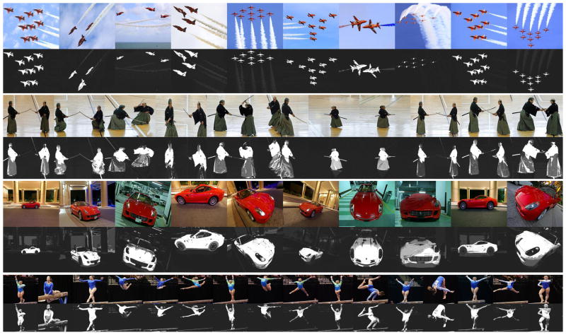
Co-saliency is used to discover the common saliency on the multiple images, which is a relatively under-explored area. In this paper, we introduce a new cluster-based algorithm for co-saliency detection. Global correspondence between the multiple images is implicitly learned during the clustering process. Three visual attention cues: contrast, spatial, and corresponding, are devised to effectively measure the cluster saliency. The final co-saliency maps are generated by fusing the single image saliency and multi-image saliency. The advantage of our method is mostly bottom-up without heavy learning, and has the property of being simple, general, efficient, and effective. Quantitative and qualitative experimental results on a variety of benchmark datasets demonstrate the advantages of the proposed method over the competing co-saliency methods, and our method on single image also outperforms most the state-of-the-art saliency detection methods. Furthermore, we apply the co-saliency method on four vision applications: co-segmentation, robust image distance, weakly supervised learning, and video foreground detection, which demonstrate the potential usages of the co-saliency map.

I. Introduction

Saliency detection could be considered as a preferential allocation of computational resources [1]–[5]. Most of existing saliency algorithms formulates on detecting the salient object from the individual image [6]–[8]. Recently, the multiple image correspondence based on a small image set has become one of the popular and challenging problems, meanwhile the co-saliency is proposed. Co-saliency detection in [9] is firstly defined as discovering the unique object in a group of similar images. However, the requirement of the similar images, captured within the same burst of shots, narrows its applications. An alternative concept is more favourite, which targets to extract the common saliency from the multiple images [10]–[12]. Extracted co-saliency map under later concept is more useful in various applications, such as co-segmentation [13]–[15], common pattern discovery [16], [17], object co-recognition [18], [19], image retrieval [20], and image summaries [21], [22]. The objective of this paper focuses on the later definition and proposes an efficient cluster-based method for detecting the common saliency on the multiple images.

Fig. 1 illustrates the co-saliency example, where the single image algorithm [3] (second row) extracts salient objects in each image, but at the cost of having confusions with the complex backgrounds. For example, the audience in the first two images highlighted by a red rectangle. Single image saliency method also lacks the relevance information on the multiple images. In contrast, our co-saliency utilizes repetitiveness property as additional constraint, and discovers the common salient object on the multiple images, e.g. the red player as shown in the bottom row of Fig. 1.

Fig. 1.

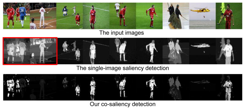
Given a group of images (first row), the state-of-the-art saliency method in [3] (second row) might be confused with complex background, and lacks the relevance information on the multiple images. In contrast with single image saliency, our co-saliency (third row) provides the recurring co-salient objects (the red player).

The goal of our work is to develop a novel cluster-based algorithm for co-saliency detection. Our method employs the clustering to persevere the global correspondence between the multiple images, and generates the final co-saliency maps by fusing three efficient bottom-up cues. A nice thing about our method is mostly bottom-up without heavy learning, and has the property of being simple, general, efficient, and effective. This paper includes the following properties: 1) we address the co-saliency definition and propose a cluster-based co-saliency detection method. 2) based on cluster-based method, a number of bottom-up cues are adopted to measure the saliency, which are originated from a well-known property of the human visual perception and multiple image information. 3) our method not only has encouraging performances on co-saliency detection, but also significantly outperforms the state-of-the-art methods on single image saliency detection. 4) at last, we present four applications, including co-segmentation, robust image distance, weakly supervised learning, and video foreground detection, to demonstrate the potential usages of the co-saliency.

This paper is organized as follows: after a brief introduction of related works in Section I-A, Section II gives the detailed implementation of our co-saliency detection method, including the two-layer clustering, the cluster-based cues, and the cue integration. Then the quantitative and qualitative experimental results on a variety of benchmark datasets are shown in Section III. Moreover, four applications of co-saliency are proposed in Section IV. Finally, some concluding remarks are presented in Section V.

A. Related Works

1) Co-saliency detection

Solutions utilizing additional companion images as cues are proved to be effective [10]–[12]. Chen [10] proposes a method to find the co-saliency between a pair of images by enhancing the similar and preattentive patches. Li and Ngan [11] model the co-saliency as a linear combination of the single image saliency map and the multi-image saliency map, by employing a complex co-multilayer graph. However, it is hard to generalize these two methods [10], [11] to the case of the multiple images. Chang et al. [12] consider the single-view saliency map and concentrate on those salient parts that frequently repeat in most images. Nevertheless, this method only defines the co-saliency as a prior for the co-segmentation task and the advantage of the co-saliency is not distinctly illuminated. Moreover, the computational requirement of [12] is very expensive. In contrast, we propose a simple yet effective cluster-based method to detect the co-saliency from multiple images. Compared with the existing techniques, our approach has a distinct advantage of being efficient and effective.

2) Co-segmentation

A closely related research area to co-saliency detection is ‘co-segmentation’, which aims to segment out the similar objects from two/multiple images [13], [14], [23]. Compared with the co-segmentation, our co-saliency detection implies a priority based on the lower level concepts, more specifically human visual attention. Furthermore, co-segmentation has three differences to co-saliency detection: First, similar but non-salient background in images could interfere the correspondence procedure for the unsupervised co-segmentation approaches [24], [25]. Second, some co-segmentation methods [14], [26] need user inputs to guide the segmentation process under ambiguous situations. Third, co-segmentation systems are often computationally demanding, especially, on a large number of images. In practice, applications such as image retargeting [27], object location and recognition [28], only need to roughly but quickly localize the common objects from the multiple images. Unlike co-segmentation, our co-saliency detection method automatically discriminates the common salient objects. Thanks to its simplicity and efficiency, our approach is able to be used as a preprocessing step for subsequent high-level image understanding tasks. Nevertheless, we evaluate the proposed co-saliency method on a number of co-segmentation datasets, finding out that, despite the lack of complex learning, the performance of our co-saliency is rather competitive with many of the recent co-segmentation methods.

II. Our Proposed Approach

As stated above, the co-saliency map can be used in various vision applications. However, co-saliency detection has not received many attentions and a limited number of the existing methods [10], [12] are not able to produce the satisfactory results. In this paper, we regard the common object to be co-saliency if it accounts the following aspects:

• (Intra-saliency) Co-saliency should follow the laws of the visually salient stimuli in the individual image, which is efficient for distinguishing salient object against the background.

• (Inter-saliency) Co-saliency exhibits high similarity on the multiple images, hence the global repetitiveness feature/distribution should be employed to highlight the common patterns.

• Furthermore, as the pre-processing step for subsequent applications, the co-saliency detection should be easy to implement and fast to compute.

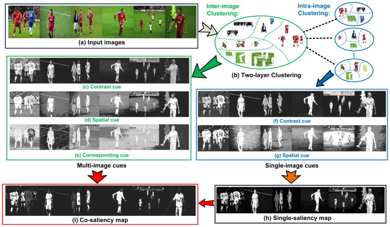
In this paper, we propose a two-layer cluster-based method to detect co-saliency on the multiple images. Fig. 2 shows the flowchart of our cluster-based method. Given a set of images, our method starts by two-layer clustering. One layer groups the pixels on each image (single image), and the other layer associates the pixels on all images (multi-image). We then compute the saliency cues for each cluster, and measure the cluster-level saliency. The measured features include the uniqueness (on single/multi-image), the distance from the image center (on single/multi-image) and the repetitiveness (on multi-image). We call them contrast, spatial, and corresponding cues, respectively. At last, based on these cluster-level cues, our method computes the saliency value for each pixel, that is used to generate the final saliency map.

Fig. 2.

The framework of our cluster-based co-saliency detection method. (a) The input images. (b) Two-layer clustering of the pixels on intra-image and inter-image. Contrast cues (c, f) and spatial cues (d, g) are extracted for both intra-image and inter-image clusters, while corresponding cues (e) is computed only for inter-image clusters. At last, the single image saliency map (h) and co-saliency map (i) are generated from these cues.

A. Cluster-based Method

The cluster-based idea is inspired by the global-contrast methods [3], [29]–[31] on the single image. These methods quantize the feature channels of pixels into the histogram format to measure the spatial contrast dissimilarity, and evaluate the saliency of the pixel with respect to the other pixels in the entire images. But the estimated feature distributions using histogram are discontinuities at the bin edges. Instead, we employ clustering to avoid the discontinuities at the bin edges of histograms, and obtain a highly cohesive global constraint. Simultaneously, clustering on the multiple images provides the global corresponding for the all images. In our method, we are not constrained to specific choice of the clustering methods, and herein K-means is used.

There are two challenges in the clustering process. How to predefine a suitable cluster number, and how much does the misclassified pixel (e.g. background pixel is grouped with saliency pixel) harm the saliency detection? Fewer clusters cause the pixels within the same cluster to have the same saliency values without sufficient discrimination. To avoid this ‘discrete’ clustering, we adopt a probability framework to smooth the co-saliency value to each pixel, which is discussed in Section II-C. And the cluster number is not the major factor for our method. The effect of the cluster number for our method with this ‘soft’ weighting is tested in Section III-D.

B. Cluster-based Saliency Cues

In this section, three cluster-based cues are introduced to measure the cluster-level saliency. The first two are contrast and spatial cues, which are previously used in the single image saliency detection. We extend these two cues into our cluster-based pipeline, and utilize them on both single image and multi-image saliency weighting. We also present a corresponding cue for discovering the common objects appearing on the multiple images. The main property of our cluster-based method is that the visual attention cues appear on cluster-level rather than the individual pixel-level. After clustering single or multiple images, the cluster-level analysis is the same between the single image and multi-image.

Notations

The pixel is denoted by ${\{p_i^j\}}_{i=1}^{N_j}$ with index i in the image I^j, where the N_j denotes the jth image lattice. ${\{z_i^j\}}_{i=1}^{N_j}$ denotes the normalized location of the pixel $p_i^j$ in the image I^j. Given M images ${\{I^j\}}_{j=1}^M$, we obtain K clusters¹ ${\{C^k\}}_{k=1}^K$. The clusters are denoted by a set of D-dimensional vectors ${\{{\mu }^k\}}_{k=1}^K$, in which μ^k denotes the prototype (cluster center) associated with the cluster C^k. And the function b: R² → {1…K} associates the pixel $p_i^j$ and the cluster index $b(p_i^j)$.

1) Contrast cue

Contrast cue represents the visual feature uniqueness on the multiple images. Contrast is one of the most widely used cues for measuring saliency in single image saliency detection algorithms [1], [3], [7], since the contrast operator simulates the human visual receptive fields. This rule is also valid in the case of cluster-based method for the multiple images, while the difference is that contrast cue on the cluster-level better represents the global correspondence than the pixel/patch.

The contrast cue w^c(k) of cluster C^k is defined using its feature contrast to all other clusters:

$$w^c(k)=\sum _{i=1,i\ne k}^K\left(\frac{n^i}{N}{\left|\right|{\mu }^k-{\mu }^i\left|\right|}_2\right),$$ (1)

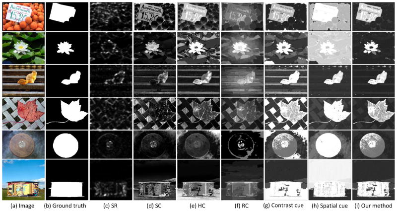
where a L₂ norm is used to compute the distance on the feature space, nⁱ represents the pixel number of cluster Cⁱ, and N denotes the pixel number of all images. This definition favours the large cluster to play more influence. The formulation (1) is similar to Histogram-based Contrast in [3]. However, there are two differences: first, [3] evaluates the saliency value using a simplified histogram, while we employ the cluster. Our cluster-based method perseveres a high coherence. Second, the contrast cue is employed only as one of three basic cues in our co-saliency method. The visual example between [3] and our contrast cue on the single image is shown in Fig. 7.

Fig. 7.

Visual comparison of single image saliency detection on MSRA1000 dataset. (a) Input image. (b) Ground truth. Saliency maps: (c) SR [6]. (d) SC [29]. (e) HC [3]. (f) RC [3]. (g) Our contrast cue. (h) Our spatial cue. (i) Our final single image saliency.

The contrast cue is valid on both single and multiple images, as shown as Fig. 2(c) and (f). The advantage of the contrast cue is that the rare clusters, e.g. the players, are intuitively more salient. However, the power of contrast cue degrades in the situation of the complex background (e.g. the audience). In addition, it does not address the locating of the common patterns on the multiple images.

2) Spatial cue

In human visual system, the regions near the image center draw more attention than the other regions [31]–[33]. When the distance between the object and the image center increases, the attention gain is depreciating. This scenario is known as ‘central bias rule’ in single image saliency detection. We extend this concept to the cluster-based method, which measures a global spatial distribution of the cluster. The spatial cue w^s(k) of cluster C^k is defined as:

$$w^s(k)=\frac{1}{n^k}\sum _{j=1}^M\sum _{i=1}^{N_j}\left[\mathcal{N}\left({\left|\right|z_i^j-o^j\left|\right|}^2\mid 0,{\sigma }^2\right)·\delta [b(p_i^j)-C^k]\right],$$ (2)

where δ(·) is the Kronecker delta function, o^j denotes the center of image I^j, and Gaussian kernel (·) computes the Euclidean distance between pixel $z_i^j$ and the image center o^j, the variance σ² is the normalized radius of images. And the normalization coefficient n^k is the pixel number of cluster C^k. Different from the single image model, our spatial cue w^s represents the location prior on the cluster-level, which is a global central bias on the multiple images.

The same as the contrast cue, the spatial cue is also valid on both single and multiple images, as shown in Fig. 2(d) and (g), where the red players located in center have higher spatial weighting than the blue players. Fig. 3 illustrates the differences between the contrast and spatial cues, where the contrast cue selects the most salient object, while the spatial cue eliminates the textured and ‘salient’ background, especially those away from the image center. On one hand, the spatial cue addresses the negative effects of the contrast cue and suppresses the confusion of complex background (e.g. the tree in first row, and the audience in second row). On the other hand, the centrally placed background (e.g. the playground in the second row) might have inaccurate spatial bias. Benefiting from both cues, our single image saliency method provides pleasing saliency maps as shown in Fig. 3(d).

Fig. 3.

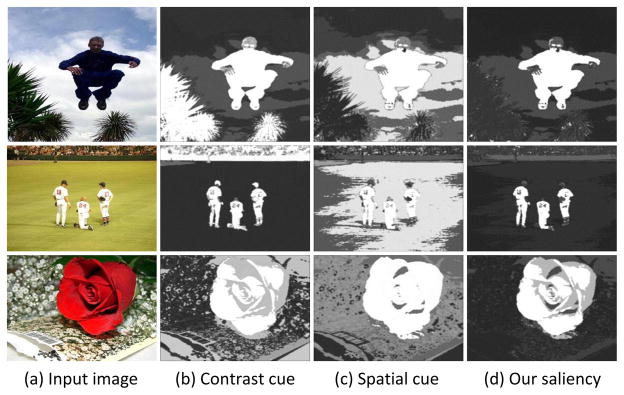
Some examples of the single image saliency detection using our contrast cue and spatial cue. (a) Input image. (b) Contrast cue is expert in discriminating the most salient object. (c) Spatial cue is good at handling the textured background around the image boundaries. (d) Our final single image saliency map joints two cues and obtains a satisfactory saliency map.

3) Corresponding cue

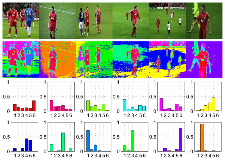
Being different from contrast and spatial cues, the third cue of our method, corresponding cue, is presented to measure how the cluster distribute on the multiple images. The repetitiveness, describing how frequent the object recurs, is an important global property of the common saliency. In fact, the clustering on inter-image approximately perseveres the global correspondence on the multiple images. Fig. 4 gives an example of clustering distribution, where the common object (e.g. the red player) distributes almost equally in each image. Based on this observation, we employ the variances of clusters to roughly measure how widely is the cluster distributed among the multiple input images.

Fig. 4.

Illustration of the corresponding cue. Top: the input image. Middle: the inter-image clustering result with cluster number K = 12. Bottom: the M-bin histogram for each cluster. These 12 clusters are ranked by their variances, where the color is corresponding the cluster in the second row. M equals the image number, i.e. 6 in this example.

Firstly, a M-bin histogram ${\widehat{\mathbf{q}}}^k={\{{\widehat{q}}_j^k\}}_{j=1}^M$ is adopted to describe the distribution of cluster C^k in M images:

$${\widehat{q}}_j^k=\frac{1}{n^k}\sum _{i=1}^{N_j}\delta [b(p_i^j)-C^k],j=1\dots M.$$ (3)

where n^k is the pixel number of cluster C^k, which enforces the condition ${\sum }_{j=1}^M{\widehat{q}}_j^k=1$. Then, our corresponding cue w^d(k) is defined as:

$$w^d(k)=\frac{1}{var({\widehat{\mathbf{q}}}^k)+1},$$ (4)

where var(q̂^k) denotes the variance of histogram q̂^k of the cluster C^k. The cluster with the high corresponding cue represents that the pixels of this cluster evenly distribute in each image.

Fig. 2(e) shows the corresponding cue, where the soccer players in red, frequently appearing in all images, have the higher distribution score than those in blue. However, the similar background also has a higher corresponding score. Thanks to the contrast and spatial cues, these background regions are discouraged in the final co-saliency maps.

C. The Co-saliency Maps

So far, three bottom-up cues in our cluster-based method are introduced². Each cue, if used independently, has its advantages and, of course, disadvantages. A common fusion is formulated as a linear summation of static salient features [1], [7]. For saliency detection, however, the precision is more important than recall [30], which prefers a more precise, rather than a large, saliency map. Therefore, we employ the multiplication operation to integrate the saliency cues. Fig. 5 illustrates the example of difference between summation and multiplication fusions. The summation generates a distribution having a heaving tail, such as the points (1, 0) and (0, 1) in Fig. 5(a). In contrast, the multiplication operation depresses the tail in Fig. 5(b) and has a more robustness for the noisy saliency pixels, as shown in Fig. 5(c).

Fig. 5.

Comparison of (a) summation and (b) multiplication fusions, where we show the 2-D transform space {x₁, x₂} ∈ [0, 1]₂ only for illustration. The multiplication is better in depressing the tails and noisy than summation. (c) The saliency map using summation and multiplication, where the multiplication effectively reduces the noisy saliency pixels caused by negative effects of each cue.

Before combining saliency cues, we normalize each cue map to standard Gaussian using the distribution of scores across all clusters. Then the cluster-level co-saliency probability p(k) of cluster k is defined as:

$$p(C^k)=\prod _i{w}_i(k),$$ (5)

where w_i(k) denotes saliency cue.

Now that the cluster-level co-saliency value is computed, which provides the discretely assignment. Then we smooth the co-saliency value for each pixel. The saliency likelihood of the pixel x belonging to the cluster C^k satisfies a Gaussian distribution as:

$$p(x\mid C^k)=\mathcal{N}({\left|\right|v_x,{\mu }^k\left|\right|}_2\mid 0,{\sigma }_k^2),$$ (6)

where v_x denotes the feature vector of pixel x, and the variance σ_k of Gaussian uses the variance of cluster Ck. Hence, the marginal saliency probability p(x) is obtained by summing the joint saliency p(C^k)p(x|C^k) over all clusters:

$$p(x)=\sum _{k=1}^{K}p(x,C^k)=\sum _{k=1}^{K}p(x\mid C^k)p(C^k).$$ (7)

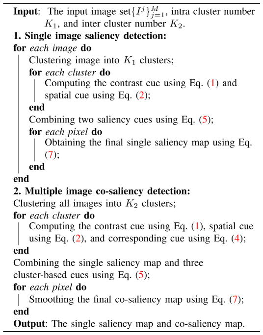
Finally, the pixel-level co-saliency is obtained, as shown in Fig. 2(i). Our method is summarized in Algorithm 1.

Algorithm 1.

Cluster-based Co-saliency Detection.

III. Experiments

We evaluate our co-saliency detection method on two aspects: the single image saliency detection, and the co-saliency detection on the multiple images. We compare our method with the state-of-the-art methods on a variety of benchmark datasets. And then a discussion is given to analyze the effectiveness of each saliency cue, the running time, and the cluster number. In the experiments, CIE Lab color and Gabor filter [34] are employed to represent the feature vector. The Gabor filter responses with 8 orientations. The bandwidth is chosen to be 1 and one scale is extracted. We compute the magnitude map of Gabor filter by combining 8 orientations as the texture feature. K-means is used in two-layer clustering. The cluster numbers in Algorithm 1 are set to K₁ = 6 for intra image (single image), and K₂ = min{3M, 20} for inter image (multiple images), where M denotes the image number.

A. Single-image saliency detection

First, we evaluate our method on the single image saliency detection. We employ the publicly available MSRA1000 saliency database provided by [30], which is the largest saliency image database (1000 images) and has pixel-level ground truth in the form of accurate manual labels. We compare our single image saliency method (SS) with five state-of-the-art detection methods: Spatiotemporal Cues (SC) in [29], Frequency-tuned saliency (FT) in [30], Spectral residual (SR) in [6], Region-based Contrast (RC) and Histogram-based Contrast (HC) in [3]. Fig. 6(a) shows the results using naive thresholding on the dataset, where the F is calculated by:

$$\text{F}-\text{measure}=\frac{(1+{\beta }^2)\text{Precision}\times \text{Recall}}{{\beta }^2\times \text{Precision}+\text{Recall}},$$ (8)

where we use β² = 0.3 as in [3], [30] to weight precision more than recall. Moreover, we also provide two individual saliency cues of our method: contrast cue (CoC) and spatial cue (SpC), as shown the dotted curves in Fig. 6(a). Our contrast cue formulates similarly to the HC [3], where ours employs the cluster instead of histogram, hence the performance of contrast cue (F = 0.755) has the similar results to the HC [3] (F = 0.751). Interestingly, the spatial cue outperforms the contrast cue, because most natural images are satisfying the central bias rule in the photography. This observation agrees with the success of the recent proposed methods [31], [32], [35]. Although the spatial cue itself can not compete with the RC [3], our cluster-based method on the single image based on the spatial and contrast cues outperforms RC [3]. And our F-measure is 0.854, which is 5% better than RC [3] (F = 0.805).

Fig. 6.

Comparison between our cluster based saliency detection methods, including the single image saliency (SS) and co-saliency (CS) methods, and other state-of-the-art works. (a) The Precision/Recall curves for naive thresholding of saliency maps on MSRA1000 dataset. We compared our work with the state-of-the-art single image saliency detection methods including RC [3], HC [3], SC [29], SR [6], FT [30]. For better understanding of the contribution of each individual cues, we also provide two curves of individual saliency cues: contrast cue (CoC) and spatial cue (SpC). (b) The Precision/Recall curves of co-saliency map on co-saliency pairs dataset. Our co-saliency detection method (CS) are compared with CO [12], MS [11] and PC [10]. (c) The Precision/Recall curves of saliency detection on iCoseg dataset.

Visual comparison of different saliency results obtained by various methods is shown in Fig. 7. For the first two images, the contrast cue contributes more than the spatial cue. However, the spatial cue still assigns the salient objects with a higher saliency score than the background. For the case of the complex and textured background or the low contrast foreground, such as the third to fifth images in Fig. 7, most existing saliency detection methods produce the failure saliency map. Since these methods only employ the low-level feature to detect saliency, they are easily harmed by the high-contrast noise on background (the third and fourth images) and low-contrast foreground (the fifth image). However, as argued before, the center bias rule, based on spatial rule instead of feature contrast, is effective for this case. And our method, which combines the contrast and spatial cues, is robust and obtains the better saliency map. In the last image in Fig. 7, contrast cue itself can not locate the salient object, since the grassland has high contrast. Spatial cue itself provides high score for the sky as this image is disobeying the central bias rule. In other words, the salient object is lower than the image center. Nevertheless, our final single image map integrates the benefits of both cues, and only the salient object, the tent, satisfies these two saliency cues.

B. Co-saliency detection

Most existing co-saliency detection methods focus on a pair of images, which are designed to detect salient objects in common. We compare our co-saliency method (CS) with three previous methods: the co-saliency by Chang et. al. (CO) in [12], the preattentive co-saliency (PC) in [10], and the multi-image saliency (MS) in [11]. The dataset uses the Co-saliency Pairs dataset [11], which includes 210 images (105 image pairs). Each image pair contains one or more similar objects with different backgrounds. Fig. 6(b) shows the Precision/Recall curves for naive thresholding on this dataset. We also offer the single image saliency methods: RC, HC in [3], and our single image method (SS), as shown the dotted curves. Similar to the observation in Section III-A, our single image method (SS) wins among all single image methods. Moreover, our SS outperforms co-saliency methods PC [10] and CO [12], and is comparable to MS [11]. The main reason is that each image inside co-saliency pairs dataset has the obvious foreground, which reduces the contribution of the second image. However, our co-saliency method still improves from the SS (F = 0.779) and MS [11] (F = 0.789) to F = 0.813.

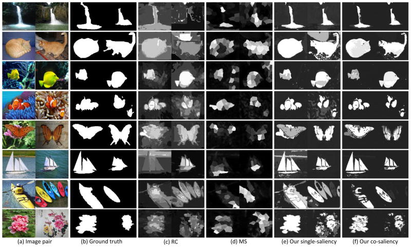
Fig. 8 shows some visual results of saliency detection on image pairs. Overall, our method provides visually acceptable saliency, which is consistent with visual attention. In the results of RC [3], highly textured backgrounds belonging to non-salient regions are not suppressed, e.g. the first two rows in Fig. 8. Relative large objects are hardly captured by MS [11] as shown in the second and fifth rows in Fig. 8. One potential reason is that MS [11] employs the local contrast of each patch and the patch size is not adaptable to the global constraint. As a result, the inside patches of large object lack salient property against their surrounding patches. In contrast, our method relieves this limitation by clustering them as one entire group, and obtains the better results on large object. Simultaneously, the complex background, such as the third and sixth images, also hurts the saliency detection in RC [3] and MS [11]. Our spatial cue provides the robustness to the complex background as same as the single image detection. Therefore our method offer the best results for the complex background. The last two pairs demonstrate the difference between the single and co-saliency detection. The single image saliency detects all the salient objects for each image. The power of co-saliency extracts the common saliency from the multiple images, such as the yellow boat and red peony.

Fig. 8.

Visual results of saliency detection on Co-saliency Pairs dataset. (a) Input image pair. (b) Ground truth. (c) Saliency map by RC [3]. (d) Saliency map by MS [11]. (e) Our single image saliency. (f) Our co-saliency.

At last, we employ the CMU Cornell iCoseg dataset [22] to test our co-saliency method on the multiple images (image number ≫ 2), which is the largest publicly available co-segmentation benchmark with 643 images in 38 groups. Since the co-saliency methods MS [11] and PC [10] are not valid on more than two images, we only compare the CO [12] and our co-saliency method (CS). The same as above, we also provide the Precision/Recall curves of the single image saliency methods: RC, HC in [3], and our single image method (SS). Fig. 6(c) shows the curves of these methods. our single image method wins among all single image methods with F = 0.699. And no surprisingly, our co-saliency method obtains the best performance on the multiple images with F = 0.732. The iCoseg dataset is provided for the co-segmentation, where the common objects may not have the bottom-up saliency properties. Therefore, the Precision/Recall scores of all methods are lower than those on co-saliency pairs dataset. Some co-saliency detection results are shown in Fig. 9, where the image set include the common salient object with non-salient background (first two samples) and complex background (last two samples). Our method obtains the accurate co-saliency maps, utilizing the overall constraints on the multiples images.

Fig. 9.

Some visual results of our co-saliency detection on iCoseg dataset. Our co-saliency map provides the accurate common object mask on the multiple images.

C. The running time

Our approach adopts the bottom-up cues to measure the co-saliency without heavy learning. Simultaneously, the cluster-based method, comparing with the individual pixel operator, achieves an efficient storage and computation. In our method, we are not constrained to specific choice of the clustering methods, and K-means is used. We randomly select the images in the same category of the iCoseg dataset with various image numbers, and resize the images with resolution 128 × 128 to evaluate the running time. Fig. 10(a) shows the cost in seconds of our entire method (red) and the clustering process (blue) running on the multiple images with cluster number K = min{3M, 20}, where M denotes the image number. The running time increases consistently with respect to the number of clusters. The experiment is run on a laptop with Dual Core 2.8 GHz processor and 4GB RAM. The code is implemented in matlab without optimization.

Fig. 10.

The analysis of our saliency map on the iCoseg dataset with various conditions. (a) The running time for various image numbers with image sizes 128 × 128 and cluster number K = min{3M, 20}, where M denotes the image number. (b) Precision/Recall curves with different saliency cues. (c) Results with various cluster numbers.

Typically, our method takes about 0.2 to 0.4 seconds for a pair of images with image size 128 × 128. The co-saliency method [12] takes about 40 and 60 seconds for generating co-saliency maps for 4 images³. The method [11] spends about 430 to 480 seconds for an image pair. Thus, our proposed method obtains a substantial improvement in running time with a competitive performance.

An other similar research to our method is co-segmentation, which extracts the pixel-level segmentation from two/multiple images. However, the computational requirements of co-segmentation are very expensive. For example, the reported running time of [23] is 4 to 9 hours for 30 images, and [12] needs 40 to 60 seconds for 4 images. In contrast, our proposed method takes only 20 to 22 mins for 300 images, and offers substantial improvements in running time under a competitive segmentation result. The more details between co-segmentation and our method are provided in Section IV-A.

D. Discussion

In this section, we discuss three factors related to our approach: The effectiveness of each saliency cue, the cluster number, and the degenerated case.

1) The effectiveness of each saliency cue

Our method employ three bottom-up cues to measure the co-saliency. To evaluate the effectiveness of each cue, we test seven Precision/Recall curves on the iCoseg dataset: co-saliency (CS), single-saliency (SS), contrast cue (CS-CoC), spatial cue (CS-SpC), and corresponding cue (CS-Corr) on multi-image, contrast cue (SS-CoC) and spatial cue (SS-SpC) on single image. From the results in Fig. 10(b), we have the following observations: (1) the saliency detection in the multi-image case (solid curves) mostly performs better than the result in the single image (dotted curves). Since the global correspondence utilizes additional companion images to constrain the saliency detection problem, and makes it easier to decide which object is the most salient one among many possible candidates. (2) The contrast cue performs similarly on the single and multi-image cases for the iCoseg dataset. This is due to the fact that the images of the same category in this dataset are captured from the similar scenes, which leads the global contrast cue on the multi-image is close to the contrast cue on the single image. (3) The spatial cue (CS-SpC) is the most useful one for this dataset, and performs even better than co-saliency (CS). This is because foreground objects in the iCoseg dataset are mostly located in the image center. However, this location prior is not always valid in practice. One example is the last row in Fig. 7. (4) The corresponding cue (CS-Corr) itself has slightly lower performance. This is expected, since the merit of the corresponding cue is to enforce the ‘common’ property on the multiple images, rather than distinguishing the saliency. In other words, the corresponding cue mainly effects on deciding which object is the common salient one among many possible candidates. Therefore, the similar backgrounds leads the corresponding cue to wrongly select the salient pixels inside those areas.

2) The cluster number

Thanks to the smoothing co-saliency value in Eq. (7), the cluster number is not the major factor in our saliency detection process. Here we only observe the cluster number of inter image clustering. We evaluate all the categories of the iCoseg dataset with various cluster numbers. Fig. 10(c) shows the performance result of saliency detection with respect to various cluster numbers. The co-saliency results in terms of precision, recall, and thus F-measure, are stable when the cluster number goes beyond 15. On the other hand, a large cluster number leads to an increasing computational requirements. Generally, we chose a loose upper bound of cluster number with K = min{3M, 20} in the experiments, where M denotes the image number.

3) The degenerated case

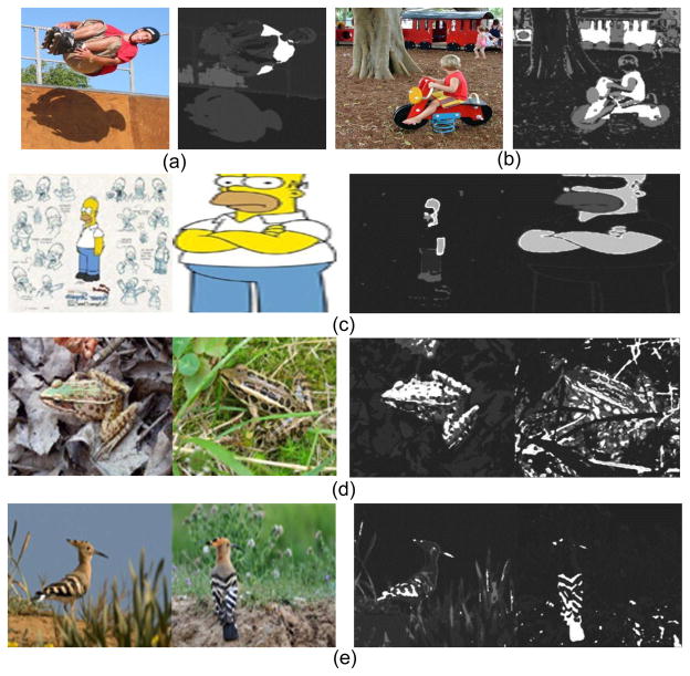
There are two degenerated cases for our saliency detection. The first case is that the object is made up by multiple components as shown in Fig. 11 (a) and (c). Our saliency method only highlights the salient component rather than the entire object. The main reason is that our saliency detection is based on bottom-up cues without heavy learning, which could not provide the object-level constraint. The second degenerated case is that the non-salient background involves the similar appearance (e.g. color) as the salient parts. Fig. 11 (b) shows this case, where the cloth of child is similar with the house in the background. This case is also caused by the protective color of animal, as shown in Fig 11 (c–d).

Fig. 11.

Some challenging examples for our saliency detection.

IV. Applications of the Co-saliency

In the past several years, the single image saliency map has been widely used in many image processing applications. However, the co-saliency is still a relatively under-explored technology. In this section, we discuss four potential applications, which benefit from the co-saliency detection results.

A. Co-segmentation

A directly related application is motivated by the recent trending of co-segmentation. Most co-segmentation task is formulated as an energy optimization problem, including a within-image energy term and a global-image energy term [13], [14], [24], [36]. These complex energy functions often cost significantly. More importantly, the co-segmentation focuses on the “similarly looking object” in a small number of images, and tends to wrongly label the “similarly background”, especially in the fully automated system. A common solution to this high level knowledge is to use manually input strokes [22], [37] or bounding boxes [38], [39]. In contrast, the co-saliency map provides an initial highlight of similarly looking object, which replaces the user interaction.

In this experiment, we utilize a bilayer segmentation method that estimates the foreground and background pixels of the input image by a Markov random field function. The energy function E is defined as:

$$E=\sum _{i\in I}p(x_i)+\sum _{\{p,q\}\in \mathcal{N}}{V}_{p,q}(x_p,x_q),$$ (9)

where x = {x_i|i ∈ I} denotes the binary-valued label of image I, p(x_i) is the co-saliency value of pixel i in Eq. (7), V_p,q is the smoothness penalty, which measures the cost of assigning different labels to two neighboring pixels, is a set of pairs of adjacent pixels. The weight V_p,q of the smoothness term is given by [40]:

$$V_{p,q}=\lambda exp(-\beta {\left|\right|z_p-z_q\left|\right|}^2),$$ (10)

where z_p is the RGB color appearance of the pixel p, β = (2〈 (z_p − z_q)²〉)⁻¹, 〈·〉 denotes expectation over the image, and λ is the weight for the contrast sensitive term. Fig. 12 shows some segmentation results using our co-saliency map. The number of images in a group of image varies from 2, 3, 4, 6 to 11. In general, we see that our co-saliency map provides an accurate saliency mask (e.g., banana and bear). In some other images, which have a shared background in some images (e.g. horse and cow), our method automatically extracts the salient foreground.

Fig. 12.

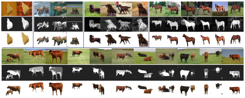
Segmentation results using our co-saliency map. First and forth rows are the input image set, the second and fifth rows are our co-saliency map, and the third and sixth rows show the segmentation results using our method.

Table I shows the quantitative comparison between our method and [12], [23] on the MSRC dataset [41]. The performance is measured by its accuracy, i.e. the proportion of correctly classified pixels (foreground and background) to the total number of pixels. The column named ‘Avg.’ in the table denotes the average score on all categories. Qualitatively, our method outperforms the co-segmentation [23] with about 8% improvement. The co-segmentation method [12] employs the co-saliency map as the prior and segments the foreground with a global energy minimization model, which improves the segmentation accuracy (Avg. = 85.95%). Our method obtains a slightly lower accuracy (Avg. = 83.55%) without any extra global energy term in Eq. 9. For the some categories, such as cat, face and bike, the common objects appear the wide range of illumination and appearance, which make our algorithm hard to group them into one cluster. This leads our method obtains the lower accuracy than [12]. However, the global energy minimization model of [12] also brings an expensive computational requirement, which needs 40 to 60 seconds for 4 images. In contrast, our method has the advantage of cheap computation, which only needs about 5 seconds to obtain the segmentation results without significantly reducing the quality.

TABLE I.

Segmentation accuracy (%) on the MSRC dataset.

Class	Plane	Cow	Cat	Face	Bike	Avg.
[23]	73.8	81.6	74.4	84.3	63.3	75.48
[12]	87.66	91.36	86.68	87.27	76.76	85.95
Our method	86.75	90.39	83.53	84.83	72.28	83.55

B. Robust Image Distance

The other interesting scenario of the co-saliency map is the robust image distance. Image visual distance measuring is a fundamentally problem and is widely employed in the reranking of image retrieval [42] and image context clustering [43]. Recently, the object sensitive image pair-distance has been demonstrated helpful to the image retrieval based on global feature comparison [13], [15], [20], [44]. For example, Rother et. al. [13] employ the co-segmentation energy as a distance measure between an image pair. However, this method is limited to its segmentation cue, which is short of a general formula for other common visual features. Inspired by [13], we provide a more efficient and general robust image distance based on the co-saliency map. The traditional visual distance between two images I₁ and I₂ is denoted by D(I₁, I₂). Given an image pair, the co-saliency segments each image into the co-saliency foreground I^f and the background I^b using Eq. (9). Then we introduce a saliency weighting rate r^f as:

$$r^f=\text{Size}(I_1^f+I_2^f)\times \text{Mean}(I_1^f+I_2^f),$$ (11)

where Size(·) and Mean(·) denote the pixel number and co-saliency mean value of foreground I^f. The background weighting rate r^b is defined by the similar way. Finally, our robust image distance D′ (I₁, I₂) based on co-saliency map is defined as:

$$D^{\prime }(I_1,I_2)=\frac{r^f}{r^f+r^b}D(I_1^f,I_2^f)+\frac{r^b}{r^f+r^b}D(I_1^b,I_2^b),$$ (12)

where

$$I_i=I_i^f+I_i^b,i=1,2.$$

Simply put, our method makes the co-saliency region (object) play the more important role in the image distance computing.

Fig. 13 illustrates some samples of comparison between the traditional distance and our robust image distance based on the co-saliency map. Our method is not limited to specific choice of the distance measure. In this experiment, color histogram Chi-squared distance is used. In the global image distance, two unrelated images have the smaller distance caused by similar backgrounds. In contrast, our robust distance focuses more on the salient objects, and relieves the affection of backgrounds. Comparing with the distance based on co-segmentation [13], [15], our proposed framework also has a favourite running time, more general form, and is easy to implement. Any distance measure can be integrated into our framework.

Fig. 13.

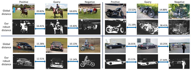
Robust image distance based on the co-saliency map. The middle image is the query image, the left image is the matched image with similar object (positive), and the right image is the unrelated image (negative) with high similar based on global color statistics. With the help of the co-saliency map, our method reduces the distance from the matched image, and increases the distance from the unrelated image.

C. Weakly Supervised Learning

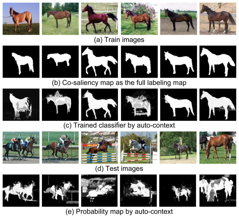
Weakly supervised learning discriminates a new object class from training images [28] with weak annotations. Different to the fully supervised scenario, the location of objects is not given. Existing approaches discover possible regions of object instances and output a set of windows containing the common object [46]–[48]. However, some classifier models need the full labeling map on pixel-level, e.g. auto-context [45]. Benefiting from our co-saliency detection, these full label classifiers could be learned without any user intervention. Fig. 14 gives an illustration of auto-context learning with our co-saliency map. Firstly, the training images are selected by weakly supervised selecting. Next, our co-saliency detection method provides the co-saliency map as the full labeling map. With the co-saliency map, the auto-context model is learned and can be used to recognize the same type of object in the challenging images as shown in Fig. 14(d).

Fig. 14.

Classifying results using our co-saliency map and auto-context [45]. (a) Training images collected by weakly supervised. (b) Our co-saliency detection map as the full labeling map. (c) Trained classifier by auto-context. (d) Test images. (e) Probability maps by auto-context recognizing

D. Video Foreground Detection

Video is treated as a sequence of images, and sometimes the foreground could be defined as the saliency object [49]–[51]. The saliency of video also conforms the feature contrast property [7], [29], [52]. Simultaneously, a reasonable assumption is that the foreground object in video may recur in the most frames, which fits the corresponding cue of the multiple images. For the spatial cue of our method, we do statistics about the position of foregrounds on video saliency dataset [50], which includes 10 videos with pixel-level ground truth. Fig. 15 shows the location map of center bias rule, where left is the estimated result on single saliency dataset [30] and right shows the result on video saliency dataset [50]. The xy-axes denote the image spacial coordinates, and the color denotes the saliency distribution of center bias map. It can be seen that the center bias rule (spatial cue) is still valid for the saliency of video, as same as the saliency of the single image. Therefore, our method could be directly used to discover the foreground on video. Fig. 16 shows the results of our co-saliency detection method on videos [53], where the foregrounds are extracted well by our co-saliency maps. Moreover, as a global corresponding on the multiple images, our method has sufficient robustness to the outlier frames, where the foreground disappears, such as the first and last frames of the second sample in Fig. 16. Note that we only use the color and texture features to cluster the pixel and extract co-saliency map. However, other spatio-temporal features, e.g. optical flow, could be easily introduced into our framework to improve the detection result on video.

Fig. 15.

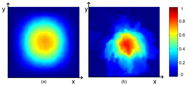
Center bias map estimation on (a) single image and (b) video. The xy-axes denote the image spacial coordinates, and the color denotes the saliency distribution of center bias map.

Fig. 16.

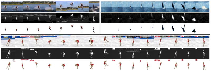
The results of foreground video segmentation using our co-saliency detection method. First and forth rows are the input video sequence, the second and fifth rows are the co-saliency map, and the third and sixth rows show the segmentation results.

V. Conclusion

In this paper, we have presented an efficient and effective cluster-based co-saliency detection method. A global association constraint could be preserved by clustering, avoiding the heavy learning. Contrast cue and spatial cues worked well for a lot datasets, since the objects in these datasets are well centered in the images and occupy a large portion of them. Corresponding cue effectively discovered the common objects on the multiple images using clustering distribution. The combined cue by multiplication obtained an encouraging results on a wide variety of datasets on both single image saliency and co-saliency detection. Our co-saliency detection, as an automatic and rapid pre-processing step, is useful for the many vision applications.

In the future, we plan to use more visual features to improve the co-saliency detection results, and investigate motion features to detect co-saliency on video. Also, it is desirable to develop saliency detection algorithms to handle the large scale dataset and object-driven system.

References

- 1.Itti L, Koch C, Niebur E. A model of saliency-based visual attention for rapid scene analysis. IEEE Trans Pattern Anal Mach Intell. 1998;20(11):1254–1259. [Google Scholar]
- 2.Lee W, Huang T, Yeh S, Chen H. Learning-based prediction of visual attention for video signals. IEEE Trans Image Process. 2011;20(11):3028–3038. doi: 10.1109/TIP.2011.2144610. [DOI] [PubMed] [Google Scholar]
- 3.Cheng M, Zhang G, Mitra NJ, Huang X, Hu S. Global contrast based salient region detection. CVPR. 2011:409–416. doi: 10.1109/TPAMI.2014.2345401. [DOI] [PubMed] [Google Scholar]
- 4.Toet A. Computational versus psychophysical bottom-up image saliency: A comparative evaluation study. IEEE Trans Pattern Anal Mach Intell. 2011;33(11):2131–2146. doi: 10.1109/TPAMI.2011.53. [DOI] [PubMed] [Google Scholar]
- 5.Valenti R, Sebe N, Gevers T. What are you looking at? improving visual gaze estimation by saliency. Int J Comput Vision. 2012;98(3):324–334. [Google Scholar]
- 6.Hou X, Zhang L. Saliency detection: A spectral residual approach. CVPR. 2007 [Google Scholar]
- 7.Liu T, Yuan Z, Sun J, Wang J, Zheng N, Tang X, Shum H. Learning to detect a salient object. IEEE Trans Pattern Anal Mach Intell. 2011;33(2):353–367. doi: 10.1109/TPAMI.2010.70. [DOI] [PubMed] [Google Scholar]
- 8.Lang C, Liu G, Yu J, Yan S. Saliency detection by multitask sparsity pursuit. IEEE Trans Image Process. 2012;21(3):1327–1338. doi: 10.1109/TIP.2011.2169274. [DOI] [PubMed] [Google Scholar]
- 9.Jacobs D, Goldman D, Shechtman E. Cosaliency: where people look when comparing images. ACM symposium on User interface software and technology. 2010:219–228. [Google Scholar]
- 10.Chen H. Preattentive co-saliency detection. ICIP. 2010:1117–1120. [Google Scholar]
- 11.Li H, Ngan K. A co-saliency model of image pairs. IEEE Trans Image Process. 2011;20(12):3365–3375. doi: 10.1109/TIP.2011.2156803. [DOI] [PubMed] [Google Scholar]
- 12.Chang K, Liu T, Lai S. From co-saliency to co-segmentation: An efficient and fully unsupervised energy minimization model. CVPR. 2011:2129–2136. [Google Scholar]
- 13.Rother C, Minka T, Blake A, Kolmogorov V. Cosegmentation of image pairs by histogram matching - incorporating a global constraint into mrfs. CVPR. 2006:993–1000. [Google Scholar]
- 14.Hochbaum D, Singh V. An efficient algorithm for co-segmentation. ICCV. 2009:269–276. [Google Scholar]
- 15.Vicente S, Rother C, Kolmogorov V. Object cosegmentation. CVPR. 2011:2217–2224. [Google Scholar]
- 16.Tan H, Ngo C. Common pattern discovery using earth mover’s distance and local flow maximization. ICCV. 2005:1222–1229. [Google Scholar]
- 17.Yuan J, Wu Y. Spatial random partition for common visual pattern discovery. ICCV. 2007 [Google Scholar]
- 18.Toshev A, Shi J, Daniilidis K. Image matching via saliency region correspondences. CVPR. 2007 [Google Scholar]
- 19.Cho M, Shin Y, Lee K. Co-recognition of image pairs by data-driven monte carlo image exploration. ECCV. 2008:144–157. [Google Scholar]
- 20.Yang L, Geng B, Cai Y, Hanjalic A, Hua XS. Object retrieval using visual query context. IEEE Trans Multimedia. 2011;13(6):1295–1307. [Google Scholar]
- 21.Goferman S, Tal A, ZelnikManor L. Puzzle-like collage. Comput Graph Forum. 2010:459–468. [Google Scholar]
- 22.Batra D, Kowdle A, Parikh D, Luo J, Chen T. Interactively co-segmentating topically related images with intelligent scribble guidance. Int J Comput Vision. 2011;93(3):273–292. [Google Scholar]
- 23.Joulin A, Bach F, Ponce J. Discriminative clustering for image co-segmentation. CVPR. 2010:1943–1950. [Google Scholar]
- 24.Mukherjee L, Singh V, Peng J. Scale invariant cosegmentation for image groups. CVPR. 2011:1881–1888. doi: 10.1109/CVPR.2011.5995420. [DOI] [PMC free article] [PubMed] [Google Scholar]
- 25.Kim G, Xing E, Fei-Fei L, Kanade T. Distributed cosegmentation via submodular optimization on anisotropic diffusion. ICCV. 2011:169–176. [Google Scholar]
- 26.Mukherjee L, Singh V, Dyer C. Half-integrality based algorithms for cosegmentation of images. CVPR. 2009:2028–2035. [PMC free article] [PubMed] [Google Scholar]
- 27.Wu H, Wang Y, Feng K, Wong T, Lee T, Heng P. Resizing by symmetry-summarization. ACM Trans Graph. 2010;29(159):1–10. [Google Scholar]
- 28.Nguyen MH, Torresani L, de la Torre F, Rother C. Weakly supervised discriminative localization and classification: a joint learning process. CVPR. 2009:1925–1932. [Google Scholar]
- 29.Zhai Y, Shah M. Visual attention detection in video sequences using spatiotemporal cues. ACM Multimedia. 2006:815–824. [Google Scholar]
- 30.Achanta R, Hemami S, Estrada F, Süsstrunk S. Frequency-tuned salient region detection. CVPR. 2009:1597–1604. [Google Scholar]
- 31.Duan L, Wu C, Miao J, Qing L, Fu Y. Visual saliency detection by spatially weighted dissimilarity. CVPR. 2011:473–480. [Google Scholar]
- 32.Tatler BW. The central fixation bias in scene viewing: Selecting an optimal viewing position independently of motor biases and image feature distributions. Journal of Vision. 2007;7(14):1–17. doi: 10.1167/7.14.4. [DOI] [PubMed] [Google Scholar]
- 33.Judd T, Ehinger K, Durand F, Torralba A. Learning to predict where humans look. ICCV. 2009:2106–2113. [Google Scholar]
- 34.Feichtinger H, Strohmer T. Gabor analysis and algorithms: Theory and applications. Birkhauser; 1998. [Google Scholar]
- 35.Liu L, Chen R, Wolf L, Cohen-Or D. Optimizing photo composition. Computer Graphic Forum. 2010;29(2):469–478. [Google Scholar]
- 36.Vicente S, Kolmogorov V, Rother C. Cosegmentation revisited: Models and optimization. ECCV. 2010:465–479. [Google Scholar]
- 37.Li Y, Sun J, Tang CK, Shum HY. Lazy snapping. ACM Trans Graph. 2004;23(3):303–308. [Google Scholar]
- 38.Rother C, Kolmogorov V, Blake A. “GrabCut”: interactive foreground extraction using iterated graph cuts. ACM Trans Graph. 2004;23(3):309–314. [Google Scholar]
- 39.Lempitsky V, Kohli P, Rother C, Sharp T. Image segmentation with a bounding box prior. ICCV. 2009:277–284. [Google Scholar]
- 40.Blake A, Rother C, Brown M, Pérez P, Torr P. Interactive image segmentation using an adaptive GMMRF model. ECCV. 2004:428–441. [Google Scholar]
- 41.Shotton J, Winn J, Rother C, Criminisi A. Textonboost for image understanding: Multi-class object recognition and segmentation by jointly modeling texture, layout, and context. Int J Comput Vision. 2009;81(1):2–23. [Google Scholar]
- 42.Deselaers T, Keysers D, Ney H. Classification error rate for quantitative evaluation of content-based image retrieval systems. ICPR. 2004:505–508. [Google Scholar]
- 43.Blaschko M, Lampert C. Correlational spectral clustering. CVPR. 2008:1–8. [Google Scholar]
- 44.Wang P, Wang J, Zeng G, Feng J, Zha H, Li S. Salient object detection for searched web images via global saliency. CVPR. 2012:3194–3201. [Google Scholar]
- 45.Tu Z, Bai X. Auto-context and its application to high-level vision tasks and 3d brain image segmentation. IEEE Trans Pattern Anal Mach Intell. 2010;32(10):1744–1757. doi: 10.1109/TPAMI.2009.186. [DOI] [PubMed] [Google Scholar]
- 46.Kim G, Torralba A. Unsupervised detection of regions of interest using iterative link analysis. NIPS. 2009:961–969. [Google Scholar]
- 47.Deselaers T, Alexe B, Ferrari V. Localizing objects while learning their appearance. ECCV. 2010:452–466. [Google Scholar]
- 48.Zhu J, Wu J, Wei Y, Chang E, Tu Z. Unsupervised object class discovery via saliency-guided multiple class learning. CVPR. 2012:3218–3225. doi: 10.1109/TPAMI.2014.2353617. [DOI] [PubMed] [Google Scholar]
- 49.Yang M, Yuan J, Wu Y. Spatial selection for attentional visual tracking. CVPR. 2007 [Google Scholar]
- 50.Ken F, Miyazato K, Kimura A, Takagi S, Yamato J. Saliency-based video segmentation with graph cuts and sequentially updated priors. IEEE International Conference on Multimedia and Expo. 2009:638–641. [Google Scholar]
- 51.Lee Y, Kim J, Grauman K. Key-segments for video object segmentation. ICCV. 2011:1995–2002. [Google Scholar]
- 52.Rahtu E, Kannala J, Salo M, Heikkil J. Segmenting salient objects from images and videos. ECCV. 2010:366–379. [Google Scholar]
- 53.Grundmann M, Kwatra V, Mei H, Essa I. Efficient hierarchical graph-based video segmentation. CVPR. 2010:2141–2148. [Google Scholar]