From simple to detailed models for cell polarization

Abstract

Many mathematical models have been proposed for the process of cell polarization. Some of these are ‘functional models’ that capture a class of dynamical behaviour, whereas others are derived from features of signalling molecules. Some mechanistic models are detailed, and therefore complex, whereas others are simplified. Each type contributes to our understanding of cell polarization. However, the huge variety at different levels of detail makes comparisons challenging. Here, we provide examples of both elementary and more detailed models for polarization. We also display how a recent mathematical method, local perturbation analysis, can provide an appropriate tool for such comparisons. This technique simplifies and speeds up the model development process by revealing the effect of model extensions, parameter variations and in silico manipulations such as knock-out or over-expression of key molecules. Finally, simulations in both one dimension and two dimensions, and particularly in deforming two-dimensional ‘cells’, can highlight behaviour not captured by traditional simulation methods.

1. Introduction

The topic of eukaryotic cell polarization has attracted the attention of many modellers, resulting in a large and growing literature. While each group has its own motivation and paradigms, some questions, on which we focus here, are of universal relevance. These include:

• — How can we hope to understand the complex networks involved in cell polarization using quantitative (modelling) approaches?

• — Can we be confident that the simplified models capture some properties well?

• — What is the relationship between detailed and stripped-down models? Do we have to use ‘functional’ models to capture the phenomena, or can we preserve some biological properties?

• — What kinds of tools can we use to study and understand models at various levels of complexity?

• — Are there reasonable methods that we can use to compare distinct models at various levels of detail?

• — What can we learn from the much more computationally intensive simulations of two-dimensional deforming cells that may not be evident in one-dimensional simulations?

All types of models have their uses and their limitations. Ultimately, we would like to be in a position to faithfully account for all the components in the complex signalling networks in the cell, and how they work together in space and time. Practically speaking, this is still a challenge for the future, as much remains to be determined experimentally before such detailed models can be constructed.

Models for cell polarity are traditionally sets of reaction–diffusion (RD) equations. These partial differential equation (PDE) models are very sensitive to changes in kinetic terms, and no universal method for classifying or categorizing their behaviour exists. This means that fully analytic comparison of distinct models is a difficult process. Simulations provide a simpler (but less satisfying) option: we can simulate various proposed models using similar protocols to see how they compare. (An example of such one-dimensional protocols was given by Jilkine & Edelstein-Keshet [1].) One issue is that each model has a variety of possible behaviours in various parameter regimes, and comparing across all models and regimes becomes combinatorially difficult. For such systems, specifically those with slow and fast diffusing components, a recent tool of local perturbation analysis (LPA) proves very helpful.

Which models are more useful, those that aim to be all-encompassing and detailed, or those that are simple and mathematically tractable? Are both types relevant to biology? Here, we argue that it is possible to preserve some biological realism in stripped-down abstract models and still refer to specific biological components. An example from our work is the activity cycling of GTPases, reviewed briefly below. Chronologically, the detailed versions of such models led to simplifications that could be analysed mathematically. In turn, the simple models were ideal for understanding the underlying mechanism at play in the tangle of interactions of the larger networks. How can we be sure that simple and detailed versions of the models preserve some common essence? Aside from simulations, it is desirable to consider the dynamic regimes that models can display as certain key parameters are varied. This type of ‘signature’ provides a summary of model dynamics that no one set of simulations adequately encompasses. We illustrate a type of bifurcation analysis that provides such a signature.

2. Models: from detailed to simple

Modelling biological systems requires a balance between detail (which implies complexity) and mathematical tractability (which motivates simplicity). These two extremes are at opposite poles of our ability to understand the implications of a model analytically. An eminent applied mathematician, Lee Segel, taught his students to seek to identify ‘which of many variables are important, and which can be disregarded in simplifying the problem’ (in the recent words of his son, Joel Segel).

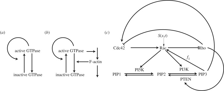
Understanding the regulatory machinery responsible for cell polarity is a prime example where this approach has been useful. While this machinery is complex and multifaceted, in many cases conserved elements and motifs emerge, as shown by the examples in figure 1. Mathematical modelling is well suited for identifying these motifs and deciphering their functions. One example is the central regulatory role of small GTPases such as Cdc42, Rac and Rho. Subsets of these regulators are ubiquitously involved in control of actin nucleation and growth, and myosin contraction in most eukaryotic cells. While their specific interactions can vary across cell types, their core function is conserved and central to eukaryotic cell motility and (in some cases) cell polarization.

Figure 1.

Schematics for a succession of simple to complex models based on reacting and diffusing components. (a) Wave-pinning (WP) model [2]. (b) The WP model is linked to F-actin via feedback, based on Holmes et al. [3]. (c) Full model of Cdc42, Rac and Rho from Holmes et al. [4, fig. 1d] (with permission of PLOS Computational Biology).

(a). Lessons we learned from small GTPase models

Models for networks of small GTPases interacting with one another and with other components have been described [5–8]. At present, there is virtually no kinetic or biochemical detail that allows each binding and regulation step to be modelled mechanistically. Moreover, attempting to do so can lead to highly complex models for small parts of the system, which are not ideal. Most such models are at least partly phenomenological. We started with the model for three interacting GTPases, Rac, Cdc42 and Rho, with mutually inhibitory interactions between the latter two and input to the central regulator Cdc42 [6, fig. 3c]. The mutual inhibition resulted in multiple steady states (bistability) with regions of high Cdc42 (front) and low Cdc42 (rear), which were at the time associated with reciprocal (low and high) Rho. However, RD models of these three interacting proteins result in waves of activity that sweep across and take over the whole cell, so no polarization can be sustained. Our first lesson from this disappointment was that not all reasonable verbal models in fact have the expected behaviour when implemented in a spatial setting. While the model displays bistable kinetics in its time-dependent version, it fails to account for the existence of multiple regions in a single spatial domain.

A second lesson we learned is that some types of biological details are important. For example, GTPases have both active and inactive forms. Transitions between these forms are on the timescale of seconds, much faster than protein synthesis, and hence the total amount is roughly constant on the timescale of cell polarity. Active GTPases are membrane-bound, and so diffuse more slowly than their cytosolic inactive counterparts. When this biological detail is incorporated [5], the model becomes a six-variable RD system with three active and three inactive forms and conservation of each of the proteins overall. While the inactive form does not participate in signalling directly, its availability affects activation: when it is depleted below some level, no further activation can take place. Incorporation of these conservative (in)activation kinetics leads to sustained polarization. Bistability initiates a wave of activity, and depletion of the inactive substrate stops this wave before it traverses the cell. This type of behaviour has been denoted wave-pinning (WP).

Another lesson gained from experience is that some modelling detail is important. For example, for simple exchange between active and inactive forms of the same protein, the basic structure of the well-mixed model (ignoring space at present) must be of the following type:

2.1

where a, b are rates of activation and inactivation that could depend on u and on other variables. In the specific case of small GTPases, a = a(u,…) is the rate of guanine nucleotide exchange factor (GEF)-mediated activation and b = b(u,…) is that of GTPase activating protein (GAP)-mediated inactivation. Both might be functions of the level of active GTPase and/or other active components that are known or hypothesized to affect (in)activation. (As v is inactive and does not participate in signalling, neither a nor b should depend on it.) In general, either a or b must be nonlinear to account for switch-like cellular responses. Moreover, it is customary to assume some saturation in the dependence of these rates on components that affect them.

One more observation that emerges from our experience is that some modelling detail is less important at this stage of exploration. Indeed, it has been shown that from a modelling perspective, numerous biochemical regulatory circuits (with positive or negative feedbacks) are functionally the same in the sense of having similar dynamic behaviour [9]. Until details about signalling systems are determined experimentally, it is therefore impossible to distinguish between (say) certain types of positive feedback to GEFs versus a specific reciprocal negative feedback to GAPs in small GTPase models. Furthermore, the switch-like response could be due to zero-order ultrasensitivity or to cooperativity (Hill functions). In future experiments, it may be possible to test for such details using knock-out experiments whereby either the GEF or the GAP is gradually silenced. At present, the choice of where the feedback acts and how it acts is, to a great extent, arbitrary in the construction of preliminary models, as they can be formally shown to be dynamically equivalent [9].

(b). Simplifying the small GTPase models

Mathematical analysis of the phenomenon of WP that we observed in the six-variable PDE model for Cdc42, Rac and Rho was challenging. In such cases, one is often constrained to exhaustive simulations (but see appendix in [6]). Consequently, it is hard to fully understand how the system works, and we were motivated to simplify and abstract this model. To do so, we formulated a prototype consisting of a single GTPase in active (u) and inactive (v) forms (resulting in a two-variable RD system). There, nonlinear positive feedback from u to its own activation replaced the previous double negative feedback. We preserved the details that had proven to be important: large differences in the rates of diffusion, constant total amount of the protein and nonlinear saturating feedback. We found that the resulting simple single-GTPase system is capable of polarizing via an apparently similar WP behaviour. The stripped-down system was then sufficiently simple to be analysed mathematically [2,10]. Interestingly, the same model was also adopted to describe polarization of PAR proteins in the early embryo of the nematode Caenorhabditis elegans [11,12]. We refer to this model henceforth as the WP model.

The significance of the WP model is as follows: first, it is a simple prototype system to describe robust polarization that has a threshold behaviour (shown below). Several recent cell motility simulations such as (e.g. [13,14]) have adopted this model to enable polarization in prototype motile cells. By construction, the WP model has aspects that specifically describe known proteins (GTPases), so it is not simply a ‘functional’ model in the sense of having appropriate dynamic behaviour. As noted in several works (e.g. [11,12]), it generalizes to signalling proteins that cycle on and off the membrane (for example, PAR proteins). Finally, its simplicity allows for extensive mathematical analysis [10], generalization to a stochastic version [15] and extension to include the effect of F-actin [3], described below.

3. Tools for analysis of polarization and other reaction–diffusion models

The vast majority of cell polarity models are based on systems of RD equations (but see Houk et al. [16], where membrane tension plays an important global inhibitory role). A unifying feature of these models is a dichotomy between fast and slow diffusing components. A typical two-variable model can be described in general by the PDEs

3.1

We will take u to be slow diffusing (D_u < D_v) and, wherever relevant, it will represent the active form of a polarity regulator. Classical analysis of such systems, dating back to Turing [17], is based on linear stability analysis (LSA) to check for instability of a homogeneous steady state (HSS) to small amplitude noise. This reduces the PDE problem (equations (3.1)) to a linear algebraic problem of determining whether eigenvalues of the linearized system can have positive real parts. When this is the case, the HSS can be destabilized and some type of pattern (spatially non-uniform solution) may result. LSA gives clues about pattern initiation and (in some cases) of the types of pattern to expect, but it cannot predict the full evolution of the system because nonlinear effects generally come into play once the perturbation grows. While LSA is an important tool in the applied mathematician toolbox, it has limitations. First, it can only check for instabilities that are provoked by arbitrarily small noise. Second, it does not easily scale up to larger nonlinear networks, where finding the HSS and eigenvalues can be extremely challenging.

For this reason, complementary tools have proved useful in our work on polarization. We review one such method, LPA, in the next section.

(a). Brief survey of local perturbation analysis

The technique described below was invented jointly by AFM Marée and V. Grieneisen. It was initially described in the appendix of Veronica Grieneisen's PhD [18], Utrecht University. It was then used extensively to parametrize models in Marée et al. [5,8] and more recently in the context of Holmes et al. [3,4]. Informal justification of this method will be presented here with detailed mathematical justification pending.

Before describing LPA, we note for future reference the typical form of kinetic equations describing the well-mixed (spatially uniform) system:

3.2

We will refer to this well-mixed system and to the full RD system (equations (3.1)).

The basic idea of the LPA is to take advantage of the diffusion discrepancy and consider the limit D_u → 0, D_v → ∞ in the RD system (equations (3.1)). We probe stability of the HSS with respect to a ‘local’ perturbation in the form of a narrow peak of u at some location in the domain. (The magnitude of the peak need not be small, but its ‘total mass’ should be negligible.) In this limit, the localized peak of u (denoted u_L) does not influence the surrounding background levels of u (denoted u_G). As v diffuses ‘infinitely fast’, it is uniform in space and can be described by a single global variable (v_G). Further, since the mass of the perturbation is negligible, u_L does not influence the evolution of v_G. So, u_G and v_G interact according to the well-mixed chemical reaction kinetics and the growth or decay of u_L is influenced by v_G.

The dynamics of this peak and the global variables describing the broader domain can then be described by a collection of evolution ordinary differential equations (ODEs) for u_L, u_G and v_G.

3.3

This system of ODEs describes the growth or decay of the stimulus peak, providing stability information for the underlying spatial system.

We now apply this method to the polarization models described above. A common feature of polarization models is interconversion between two forms with the total average concentration w conserved. We show two such examples below. In this case, g(u,v) = −f(u,v). We use conservation,

to eliminate one variable (v_G in this case), leaving the reduced LPA system

3.4

The original problem consisting of PDEs has been reduced to a set of ODEs describing the growth of a narrow pulse. Dynamics of these ODEs under a wide range of parameter variation can be explored readily using bifurcation software.

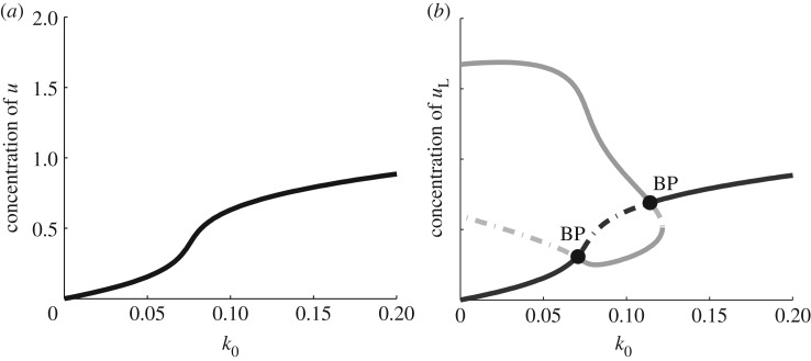
Figure 2 depicts the results of such an analysis. For the given parameter set, the well-mixed WP model has a unique stable steady-state value of u for all values of the parameter k₀, as shown in figure 2a. As k₀ increases, the steady-state level of the active form u increases monotonically. We refer to this curve as the ‘global branch’ in what follows. As shown in figure 2b, the LPA diagram includes both the global branch and an additional (grey) curve hereafter denoted the ‘local branch’. The interpretation of this LPA diagram will be explained in the next section, where a comparison with a second model is made.

Figure 2.

(a) Bifurcation diagram of the well-mixed WP system (equation (3.2)) with the kinetics (equation (4.1)). The steady-state value of u is plotted with respect to a basal activation rate, k₀. Parameter values n = 2, γ = 1, u₀ = 1, δ = 1 and total average concentration w = 2.2683. (b) LPA diagram of the WP system (same parameter values). This diagram forms a ‘signature’ for the model. It also provides information about distinct behaviours possible in various parameter regimes. BP indicates a branch point bifurcation. See text for details.

LPA has several benefits. It is fairly easy to formulate the LPA ODEs by identifying the slow and fast variables. It is then easy to explore the parameter regimes of growth/decay and/or threshold behaviour of the perturbation using bifurcation software. Below, we further illustrate several advantages of LPA. (i) It provides a standardized tool for comparison of distinct RD models for polarization. (Models with similar mechanisms have a similar LPA ‘signature’. Models that look superficially similar but have distinct mechanisms have different LPA signatures.) (ii) LPA helps to point to what changes when a model is extended or modified in some way. For example, if new feedback in introduced or another component is added to a model, then LPA can show how the behaviour changes over a whole range of parameter variation. (iii) LPA is relatively easy to scale up to larger systems of interacting components. This makes LPA much more ‘user-friendly’ than LSA.

4. Model comparisons

As previously mentioned, the literature on models for cell polarization is large, with a variety of models of many types [19–21]. How should we compare such models and their functionality? In principle, we can do so by simulating the response of models to similar protocols [1], but this can at best probe a limited set of parameters in each case. Here, we show that LPA can help to inform such comparisons.

(a). Example 1: comparison of wave-pinning and Otsuji models

Here, we use LPA to compare the polarization model of Otsuji et al. [19] (abbreviated OT) to the WP model of Mori et al. [2]. Both OT and WP share the form of equations (3.1) with g(u,v) = −f(u,v), implying conservation of the total amount of protein. In both models, u and v represent active and inactive forms of GTPases, respectively. The kinetics for these models are given by, for the WP model [2]

4.1

and for the OT model [19]

4.2

In the kinetics of equation (4.1), there is a rate of activation of u from v (basal value k₀) and an inactivation rate δ. (This follows the form of equations (2.1).) A Hill function depicts positive feedback from u to its own activation. The total average concentration, w, is determined by initial conditions, not by other parameters. While OT kinetics (equation (4.2)) can be rewritten similarly in the form of equations (2.1), both activation and inactivation rates depend explicitly on the total average amount of protein w.

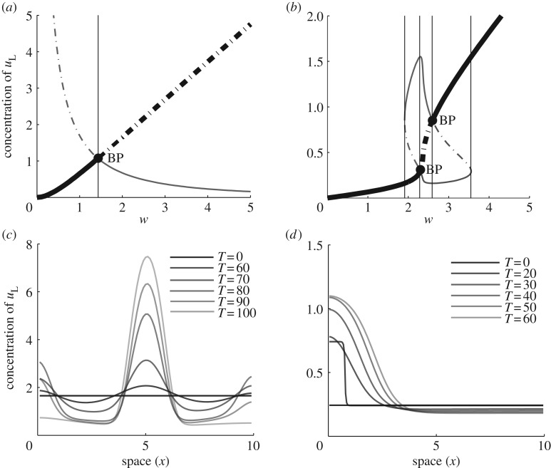
Figure 3 compares the LPA ‘signatures’ of WP and OT. Here, the steady-state value of u_L is plotted against the bifurcation parameter w. In each case, there is a monotonically increasing ‘global branch’ (thick dark curve), together with an additional ‘local branch’ that stems from spatial features captured by the LPA equations (thinner grey curve). The OT model in figure 3a has a strictly decreasing local branch. For small values of w, only the global branch is stable. The intersection point is a transcritical (branch point) bifurcation at which the two branches exchange stability. Thereafter, for larger w values, we have a Turing regime, whereby a perturbation of arbitrarily small size can lead to patterning. To the left of that bifurcation, LPA suggests that only perturbations of sufficiently large amplitude might lead to destabilization. (In practice, because LPA is an asymptotic approximation, and as the local branch climbs very steeply upwards towards the left, it is hard to cause patterning in that regime.)

Figure 3.

A comparison of LPA diagrams for (a) Otsuji [19] and (b) WP [2] models, showing u_L with the total average concentration and w as the bifurcation parameter. (a) Otsuji kinetics (equation (4.2)) with a₁ = 25, a₂ = 0.7. There is a single bifurcation at w = 1.429. (b) WP kinetics (equation (4.1)) with k₀ = 0.067, γ = 1, u₀ = 1, δ = 1, n = 2. Bifurcations are at branch points (transcritical): w = 2.3, 2.6; limit points (fold): w = 1.91, 3.55. The behaviour of the model can be classified into regimes (separated by thin vertical lines): Region I: 0 < w < 1.91, II: 1.91 < w < 2.3, III: 2.3 < w < 2.6, IIb: 2.6 < w < 3.55 and IV: 3.55 < w. BP indicates a branch point bifurcation. (c,d) A series of spatial profiles at increasing times T of the full RD PDEs for (c) the Otsuji kinetics (equation (4.2)) with w = 2 in the Turing regime (patterning initiated by numerical noise) and (d) the WP kinetics (equation (4.1)) with w = 2.2 demonstrating wave-pinning behaviour (a pulse at t = 20 initiates patterning).

Figure 3b for the WP model is significantly different. First, we see four rather than two major regions (I–IV, left to right, see legend of figure 3). In Regions I and IV, a stable HSS can never be perturbed. In Region II, the HSS is stable (solid curve) but can be destabilized by a sufficiently large local perturbation (past the threshold of the local branch, dot–dashed). For values of w between the two intersections (transcritical bifurcations), the HSS is unstable to any perturbation (Turing regime, Region III). Between the rightmost intersection and the ‘knee’ to its right, the system can only be prodded away from its elevated HSS by a pulse that locally lowers the value of u by a sufficient amount (Region IIb). It turns out that both Regions II and IIb correspond to wave-pinning behaviour, a fact that can only be determined by full-scale simulations. Examples of full PDE simulations in one spatial dimension are shown in figure 3c for OT and figure 3d for WP. In general, OT tends to form steep peaks, whereas WP has plateaus with broad shoulders.

In short, WP has distinct regimes of (i) complete stability, (ii) Turing instability and (iii) two distinct regimes of threshold response. OT shares the Turing regime, and a threshold response that in practice proves hard to trigger. Overall, aside from providing insight into parameter regimes for a given model, LPA produces a graphical summary of the range of distinct dynamic properties, providing a ‘signature’ that can be compared across RD polarization models.

(b). Example 2: the effect of model extension and additional feedback

The WP model has been studied earlier in Mori et al. [2,10] and by LPA and related methods in Walther et al. [15]. Here, we show that LPA can be used to understand the effects of model extension or modification. In Holmes et al. [3], we considered an extension of the WP model that included interaction with F-actin (see figure 1b). This was motivated by the following observations: (i) waves of F-actin and nucleation promoting factor activity have been observed in cells [22–24] and (ii) waves of small GTPases and edge protrusion (presumably powered by actin polymerization) have also been observed [25]. Accordingly, a modified WP model was linked to nucleation of F-actin. Feedback from F-actin was assumed to accelerate inactivation of the small GTPase (figure 1b), that is, to act as negative feedback channelled through GAPs. The resulting WP-F model is among the simplest descriptions of F-actin waves driven by nucleation promoting factors.

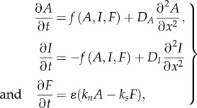
To account for the additional influence of F-actin (F) on the system, the following minimal extension of the WP model is used

4.3

where the GTPase kinetics includes an F-actin-dependent inactivation term

4.4

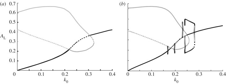
The model was explored by simulations guided by LPA analysis [3]. Figure 4 compares the bifurcation diagrams for the WP model alone (where F is treated as a constant parameter, i.e. ε = 0) and the fully dynamic A, I, F model. We see the appearance of several new Hopf bifurcations that were absent in WP, arising as a result of the dynamic feedback from F-actin. These regimes lead to a variety of wave-like behaviours [3], including static polarization, oscillatory polarization, travelling wave trains, reflecting waves and other exotic patterns as shown in figure 5. Note that such wave-like patterns are absent in the WP model alone.

Figure 4.

LPA bifurcation diagram reveals the effect of model extension from WP to WP-F (figure 1a,b). (a) WP system alone, showing active GTPase A_L versus basal activation rate k₀. Here, F-actin is treated as a parameter (F = 5) in the system (equations (4.3)) with kinetics f(A,I,F) given by equation (4.4). Transcritical bifurcations occur at k₀ = 0.2178, 0.3051 (branch points) and fold bifurcation at k₀ = 0.3229 (limit point). (b) As in (a) but with F-actin as a dynamic variable. Note new Hopf bifurcations at k₀ = 0.169, 0.1963, 0.2318, 0.2419, 0.2799. (The outer two of these are on the global branch.) These indicate presence of oscillatory behaviour. Transcritical bifurcations are seen at k₀ = 0.1814, 0.25, and there is a fold bifurcation at k₀ = 0.2586. Parameters values: A₀ = 0.4, γ = 1.0, s₁ = 0.7, s₂ = 0.7, T = 1, ε = 0.1, k_n = 2.0, k_s = 0.25.

Figure 5.

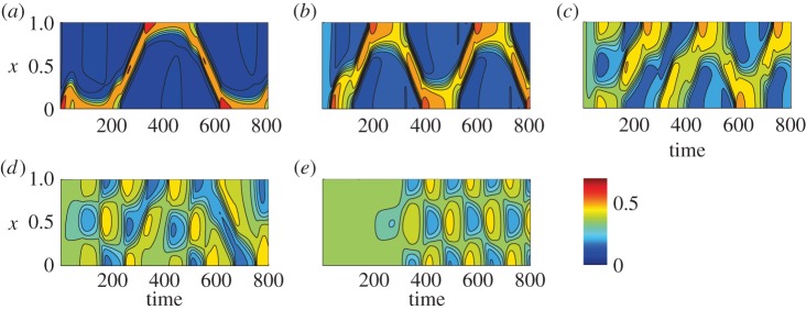
Full simulations of the WP-F model (equations (4.3) and (4.4)) showing A(x,t). A variety of waves and periodic travelling patterns are obtained. Parameter values as in figure 4b, with (a) k₀ = 0.1, (b) k₀ = 0.175, (c) k₀ = 0.22, (d) k₀ = 0.24, and (e) k₀ = 0.25.

5. Comparing simple and detailed models for polarization

Ultimately, we are interested in learning about real signalling networks and their dynamic behaviours. To do so, we must return to the more complex biological scenarios, where GTPases interact with each other and with other signalling modules. A benefit of this approach is that the model components are linked to known molecules which could, in principle, be manipulated in experimental tests.

Examples of this type of modelling include Dawes & Edelstein-Keshet [7], Marée et al. [8], Kholodenko [9] and Marée et al. [26]. In Kholodenko [9] and Marée et al. [26], models for active and inactive Cdc42, Rac and Rho were simulated spatially in one dimension and two dimensions, in both static and deforming ‘cells’. In Dawes & Edelstein-Keshet [7], Marée et al. [8], GTPases were linked to phosphoinositides PIP, PIP₂ and PIP₃ via positive feedback to/from Rac and Cdc42. (The role of PIPs has been controversial in the biological literature, and we sought to explore how they affect the small GTPase layer.) These models were based on mutual inhibition between Cdc42 and Rho supplemented by positive feedback from Cdc42 to Rac and from Rac to Rho.

In recent experimental work described by Lin et al. [27], HeLa cells cultured in microfluidic chambers were highly constrained to polarize along the direction of narrow channels. Biochemical constructs in these cells were engineered to convert a controlled external gradient of a small molecule (rapamycin) into a robust internal gradient of Rac, bypassing all the innate receptor-based signalling systems. Cells in several states were tested for polarization responses, and results were quantified and compared to a sequence of models for internal signalling. We noted immediately that the model based on mutual antagonism between Cdc42 and Rho could not account for the Rac-mediated polarization response: in fact, that model polarizes in a direction opposite to the gradient of Rac activation. Rather than simply add supplemental interactions to an existing set of proposed interactions, we instead sought the simplest connectivity between these GTPases capable of recapitulating this data. Figure 1c shows the schematic diagram of this ‘minimal circuit’. See Holmes et al. [4] for details of the models and analysis.

The level of complexity of the detailed network in figure 1c is significantly greater than that of the WP model in figure 1a: the model consists of nine PDEs (for C, R, ρ active/inactive forms, and P₁, P₂, P₃ representing the three forms of PIP lipids.) However, carrying out LPA analysis is relatively straightforward, because the resulting 15 LPA-ODEs (PIP_1,2,3 are considered slow variables) are simpler to analyse with bifurcation software than most systems of even two to three nonlinear PDEs.

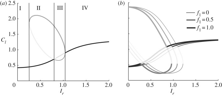
A typical LPA bifurcation plot with respect to the basal activation rate for Rac (I_r) leads to the diagram shown in figure 6a. A direct comparison can be made with figure 2b which provides the LPA diagram for WP with respect to a similar basal activation rate parameter k₀. We observe a number of similarities: both models share a monotonically increasing global HSS branch (dark curves). Both share similar regimes: a wave-pinning polarization regime where the HSS is sensitive to a sufficiently large stimulus peak (II), a Turing noise-sensitive regime (III) and a regime where no perturbation induces patterning and only the HSS is stable (IV). It is interesting to note that, even though the models are significantly different, they share certain key features. (This suggests that lurking behind a facade of details is the core mechanism that was identified in the far simpler WP model.) Furthermore, these similarities are easily detected using the LPA.

Figure 6.

(a) LPA bifurcation diagram of the models shown in Holmes et al. [4, fig. 1c]. The value of Cdc42 C_l is plotted versus a basal Rac activation rate I_r. (b) Same diagram showing the effect of feedback from the PIPs to Rac. Adapted from [4, figs 3 and 6a] with permission of PLOS Computational Biology.

A second feature of figure 6 illustrates the usefulness of the LPA diagram in understanding the effect of specific experimental manipulation. Figure 6b shows the effect of PI3K knock-out, which reduces the feedback between PIP₃ and Rac (marked with f₁ in figure 1c). The series of increasingly thick curves represent increasing levels of feedback (from none at f₁ = 0 to essential at f₁ = 1). As feedback increases, the grey loop (‘local branch’) shifts to the left. This means that at a given value of the activation rate k₀, the cell is more sensitive to stimulation: a pulse of smaller amplitude is able to breach the threshold and lead to polarization. In this sense, LPA also illustrates how feedbacks of various sorts affect cell behaviour, with minimal computational effort.

6. Cell shape and model comparisons

The ultimate test of polarization models is how they perform in a deforming cell, and how they are linked to cell motility. In real cells, assembly of the cytoskeletal polymer actin prods the cell membrane forward at the leading edge, while contraction of the cytoskeleton by myosin molecular motors pulls up the rear. Anchorage by adhesion molecules provides requisite traction. Cell polarity is an additional layer of chemistry that keeps cell migration oriented.

The simplest possible model for a deforming cell requires only a recipe that couples intracellular chemistry to membrane velocity. To focus on the interaction between cell shape and cell polarity, it makes sense to bypass a detailed description of molecular force generation by coupling the chemical kinetics of cell polarity directly to membrane displacement. This phenomenological approach allows for a direct comparison of different polarity mechanisms, without additional complicating factors.

(a). Level set methods

Investigating the influence of cell geometry on cell polarity requires a scheme for describing arbitrary cell shapes. One possibility would be a Lagrangian description of points along a parametrized cell boundary. Level set methods provide an Eulerian alternative. As a simple example, in two dimensions, consider a circular cell that grows bigger, without changing shape. Level set methods describe this scenario in terms of a cone that points downwards as it descends along a vertical axis. Intersection of this moving cone with a fixed horizontal plane then represents the edge of the growing cell. At any point in the plane, the corresponding cone elevation ψ gives the shortest distance to the cell boundary, with negative elevations inside. This defines a ‘distance map’ for which the zero level set (ψ = 0) provides an implicit description of the cell boundary. In general, once intracellular physics sets the velocity V for membrane displacement, advection of ψ then moves the boundary appropriately (∂ψ/∂t = − V · ∇ψ), using standard (though non-trivial) numerical methods [28,29]. Level set methods make it easy to compute the outward normal and curvature κ of a cell boundary ( and ).

(b). The moving boundary node method

Given a level set description for the edge of a cell, it remains to describe cell polarity within the contained region. The moving boundary node method [30] provides a means of solving the requisite differential equations. In a level set representation, the cell boundary usually falls between the nodes of a computational grid, with the boundary location determined by interpolation. However, nodes near the boundary can be moved onto the boundary without difficulty; taken together, ψ and give exactly the required displacements. This yields dynamic, boundary-fitted coordinates and a set of distorted volume elements that exactly fit the shape of a cell. Computational nodes retain simple Cartesian connectivity, which makes it easy to compute fluxes between adjacent volume elements. This leads to a finite-volume discretization of reaction–advection–diffusion equations inside moving, deforming cells. The method is accurate to second order and conserves mass.

(c). Comparison of wave-pinning and Otsuji polarity

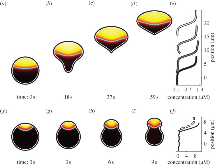
For both the Turing regime of OT (figure 3a) and region II of WP (figure 3b), perturbation of an unstable, spatially homogeneous steady state triggers polarization of a static circular cell. Disrupting the homogeneity of active protein u with a 10% spatial gradient across the cell provides sufficient stimulus. Compared with WP (figure 7a), polarization for OT (figure 7f) is more localized and has a peak of greater magnitude. These polarized states, for static cells, provide initial conditions for cells with moving boundaries.

Figure 7.

For default parameters (figure 3b), simple coupling of WP to cell boundary velocity (equation (6.1)) yields transient deformation (b,c), followed by steady translation (from (e) onwards), starting from a fully polarized circular cell (a). Boundary motion for OT with default parameters (figure 3a) yields rapid constriction (g–i) without significant translation. Concentration profiles along the vertical symmetry axis of each cell are shown for the WP case (e), whereas only the initial (solid) and final (dashed) profiles are shown for the OT case (j). For each cell, the polymerization threshold u* is shown as a cyan contour.

Perhaps the simplest possible assumption is a linear relationship between the concentration of active protein, u, and velocity, v, along outward normal, , at each point on the perimeter of a cell

6.1

where V₀ = 0.5 µm s⁻¹ sets a realistic velocity for typical crawling cells, while u_SS is the steady-state concentration for a polarized, static, circular cell, and u* is an outward growth threshold, chosen here as the value of u_SS at which |∇u_SS| attains a maximum. Points on the cell boundary where u − u* is positive move outward, along , whereas the cell contracts at points where u − u* is negative. For the same parameter values considered in one dimension (figure 3), WP yields convex, translating cells (figure 7b–d), whereas OT yields constricting, concave cells (figure 7g–i).

Constriction of cells under OT can be understood as dominance of reactions over diffusion. This can be expressed as a ratio of timescales

6.2

where τ_R is the characteristic time for OT reactions while R = 5 µm is the chosen cell radius, so τ_D is the characteristic time for intracellular diffusion. Recall that a₁ is the reaction rate for OT (equation (4.2)), whereas k₀, δ and γ are WP reaction rates (equation (4.1)). Substituting the maximum of k₀, δ or γ for a₁ in τ_R gives the characteristic time for WP reactions instead. For either OT (figure 7g–i) or WP (figure 8d,e), a ratio of τ_D/τ_R = 2500 yields constriction. In this case, relatively fast reactions cause localized depletion of u that diffusion fails to replenish so u drops below u* to give inward velocity at the point of concavity. By contrast, a ratio τ_D/τ_R = 250 yields convex translating cells for both WP (figure 7a–d) and OT (figure 8d,e).

Figure 8.

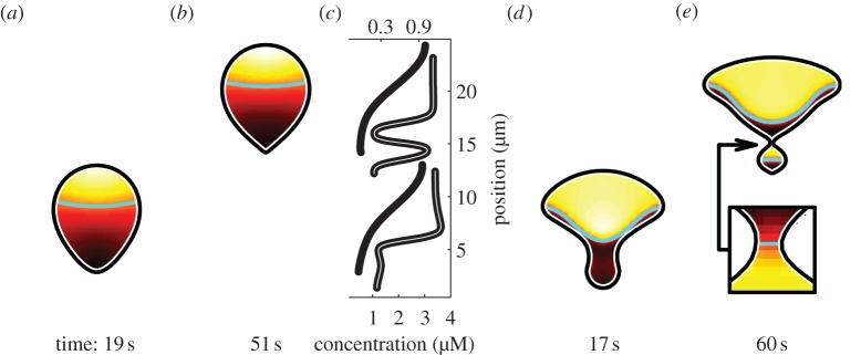
Unconstricted, convex cells (a,b), result when the default reaction rate for OT is replaced with a lower value (a₁ = 1 s⁻¹). Constricted, concave cells (e,f) result when default WP reaction rates are replaced with higher values (δ = γ = 5 s⁻¹). Concentration profiles along the vertical symmetry axis of each cell (c) use different scales, with concentrations for WP (black curves) along the top edge of the graph and concentrations for OT (grey curves) along the bottom. For each cell, the polymerization threshold u* is shown as a cyan contour.

Notably, constriction under WP (figure 8d,e) highlights some limitations of working in one dimension. In two dimensions, the cell develops a narrow bottleneck (figure 8e, inset) between two compartments. The width of the bottleneck and the average radius of each compartment give a constricted cell three inherent length scales, compared to the single length scale for polarity simulations in one dimension (figure 3). This is significant because the trade-off between reaction and diffusion timescales (equation (6.2)) depends on the characteristic length of the region in question. These geometrical effects somehow combine to manifest as emergence of two separate regions in which u is elevated (figure 8e), starting from just one region (figure 7a). Over time, the concentration profile for constriction under WP develops a local maximum, towards the rear of the cell (figure 8c, grey curves). This does not happen in one dimension (figure 3d), for a comparable initial condition.

7. Discussion

In this paper, the main emphasis has been on GTPase-based models for polarity initiation in motile eukaryotic cells. The models surveyed here consist of sets of RD equations. We have shown several methods for comparing across distinct models (from simple abstract ones to more detailed and complex ones). One method that is of particular utility is the LPA, a useful tool for systems with slow and fast rates of diffusion. We have shown that seemingly related models for polarization in fact have very different LPA ‘signatures’ (as shown in figure 3 for two types of small GTPase models), whereas models at different levels of detail can be related by a common or similar LPA signature (e.g. figures 2b and 6a.)

LPA can complement other methods of analysis but is not a replacement for full-scale simulations, such as those of figures 3c,d and 5. Those are still needed to explore the patterns that form after the short-time initiation phase. A first step is to determine the behaviour of such models in one-dimensional spatial domains where we can ask whether robust polarization results from various stimuli.

However, as shown in §6, even full-scale one-dimensional simulations are not always predictive of the evolution of polarization in a deforming two-dimensional ‘model cell’. While the latter defines a challenging moving boundary problem, such simulations are an ultimate test of models for polarization and cell motility.

Funding statement

The authors acknowledge support from NSERC discovery grant to L.E.K. and NSERC postgraduate fellowship to M.D. L.E.K. and W.R.H. have also been partly supported by National Institutes of Health under grant no. R01 GM086882 to Anders Carlsson.

References

- 1.Jilkine A, Edelstein-Keshet L. 2011. A comparison of mathematical models for polarization of single eukaryotic cells in response to guided cues. PLoS Comput. Biol. 7, e1001121 (doi:10.1371/journal.pcbi.1001121) [DOI] [PMC free article] [PubMed] [Google Scholar]
- 2.Mori Y, Jilkine A, Edelstein-Keshet L. 2008. Wave-pinning and cell polarity from a bistable reaction–diffusion system. Biophys. J. 94, 3684–3697 (doi:10.1529/biophysj.107.120824) [DOI] [PMC free article] [PubMed] [Google Scholar]
- 3.Holmes W, Carlsson A, Edelstein-Keshet L. 2012. Regimes of wave type patterning driven by refractory actin feedback: transition from static polarization to dynamic wave behaviour. Phys. Biol. 9, 046005 (doi:10.1088/1478-3975/9/4/046005) [DOI] [PMC free article] [PubMed] [Google Scholar]
- 4.Holmes W, Lin B, Levchenko A, Edelstein-Keshet L. 2012. Modelling cell polarization driven by synthetic spatially graded Rac activation. PLoS Comput. Biol. 8, e1002366 (doi:10.1371/journal.pcbi.1002366) [DOI] [PMC free article] [PubMed] [Google Scholar]
- 5.Mareé AF, Jilkine A, Dawes A, Grieneisen VA, Edelstein-Keshet L. 2006. Polarization and movement of keratocytes: a multiscale modelling approach. Bull. Math. Biol. 68, 1169–1211 (doi:10.1007/s11538-006-9131-7) [DOI] [PubMed] [Google Scholar]
- 6.Jilkine A, Marée AFM, Edelstein-Keshet L. 2007. Mathematical model for spatial segregation of the Rho-family GTPases based on inhibitory crosstalk. Bull. Math. Biol. 69, 1943–1978 (doi:10.1007/s11538-007-9200-6) [DOI] [PubMed] [Google Scholar]
- 7.Dawes A, Edelstein-Keshet L. 2007. Phosphoinositides and Rho proteins spatially regulate actin polymerization to initiate and maintain directed movement in a 1D model of a motile cell. Biophys. J. 92, 744–768 (doi:10.1529/biophysj.106.090514) [DOI] [PMC free article] [PubMed] [Google Scholar]
- 8.Marée A, Grieneisen V, Edelstein-Keshet L. 2012. How cells integrate complex stimuli: the effect of feedback from phosphoinositides and cell shape on cell polarization and motility. PLoS Comput. Biol. 8, e1002402 (doi:10.1371/journal.pcbi.1002402) [DOI] [PMC free article] [PubMed] [Google Scholar]
- 9.Kholodenko B. 2006. Cell-signalling dynamics in time and space. Nat. Rev. Mol. Cell Biol. 7, 165–176 (doi:10.1038/nrm1838) [DOI] [PMC free article] [PubMed] [Google Scholar]
- 10.Mori Y, Jilkine A, Edelstein-Keshet L. 2011. Asymptotic and bifurcation analysis of a wave-based pattern formation mechanism in a model of cell polarization. SIAM J. Appl. Math. 71, 1401–1427 (doi:10.1137/10079118X) [DOI] [PMC free article] [PubMed] [Google Scholar]
- 11.Goehring NW, Hoege C, Grill SW, Hyman AA. 2011. PAR proteins diffuse freely across the anterior–posterior boundary in polarized C. elegans embryos . J. Cell Biol. 193, 583–594 (doi:10.1083/jcb.201011094) [DOI] [PMC free article] [PubMed] [Google Scholar]
- 12.Goehring NW, Trong PK, Bois JS, Chowdhury D, Nicola EM, Hyman AA, Grill SW. 2011. Polarization of PAR proteins by advective triggering of a pattern-forming system. Sci. Signal. 334, 1137–1141 (doi:10.1126/science.1208619) [DOI] [PubMed] [Google Scholar]
- 13.Wolgemuth C, Stajic J, Mogilner A. 2010. Redundant mechanisms for stable cell locomotion revealed by minimal models. Biophys. J. 98, 160a–161a (doi:10.1016/j.bpj.2009.12.864) [DOI] [PMC free article] [PubMed] [Google Scholar]
- 14.Shao D, Levine H, Rappel W. 2012. Coupling actin flow, adhesion, and morphology in a computational cell motility model. Proc. Natl Acad. Sci. USA 109, 6851–6856 (doi:10.1073/pnas.1203252109) [DOI] [PMC free article] [PubMed] [Google Scholar]
- 15.Walther GR, Marée AF, Edelstein-Keshet L, Grieneisen VA. 2012. Deterministic versus stochastic cell polarisation through wave-pinning. Bull. Math. Biol. 74, 2570–2599 (doi:10.1007/s11538-012-9766-5) [DOI] [PMC free article] [PubMed] [Google Scholar]
- 16.Houk AR, Jilkine A, Mejean CO, Boltyanskiy R, Dufresne ER, Angenent SB, Altschuler SJ, Wu LF, Weiner OD. 2012. Membrane tension maintains cell polarity by confining signals to the leading edge during neutrophil migration. Cell 148, 175–188 (doi:10.1016/j.cell.2011.10.050) [DOI] [PMC free article] [PubMed] [Google Scholar]
- 17.Turing A. 1952. The chemical basis of morphogenesis. Phil. Trans. R. Soc. Lond. B 237, 37–72 (doi:10.1098/rstb.1952.0012) [DOI] [PMC free article] [PubMed] [Google Scholar]
- 18.Grieneisen V. 2009. Dynamics of auxin patterning in plant morphogenesis. PhD thesis, University of Utrecht, Utrecht, The Netherlands [Google Scholar]
- 19.Otsuji M, Ishihara S, Co C, Kaibuchi K, Mochizuki A, Kuroda S. 2007. A mass conserved reaction–diffusion system captures properties of cell polarity. PLoS Comput. Biol. 3, e108 (doi:10.1371/journal.pcbi.0030108) [DOI] [PMC free article] [PubMed] [Google Scholar]
- 20.Levchenko A, Iglesias P. 2002. Models of eukaryotic gradient sensing: application to chemotaxis of amoebae and neutrophils. Biophys. J. 82, 50–63 (doi:10.1016/S0006-3495(02)75373-3) [DOI] [PMC free article] [PubMed] [Google Scholar]
- 21.Goryachev A, Pokhilko A. 2008. Dynamics of Cdc42 network embodies a Turing-type mechanism of yeast cell polarity. FEBS Lett. 582, 1437–1443 (doi:10.1016/j.febslet.2008.03.029) [DOI] [PubMed] [Google Scholar]
- 22.Gerisch G, Bretschneider T, Müller-Taubenberger A, Simmeth E, Ecke M, Diez S, Anderson K. 2004. Mobile actin clusters and traveling waves in cells recovering from actin depolymerization. Biophys. J. 87, 3493–3503 (doi:10.1529/biophysj.104.047589) [DOI] [PMC free article] [PubMed] [Google Scholar]
- 23.Gerisch G. 2010. Self-organizing waves that simulate phagocytic cup structures. PMC Biophys. 3, 7 (doi:10.1186/1757-5036-3-7) [DOI] [PMC free article] [PubMed] [Google Scholar]
- 24.Weiner O, Marganski W, Wu L, Altschuler S, Kirschner M. 2007. An actin-based wave generator organizes cell motility. PLoS Biol. 5, 2053–2063 (doi:10.1371/journal.pbio.0050221) [DOI] [PMC free article] [PubMed] [Google Scholar]
- 25.Machacek M, et al. 2009. Coordination of rho GTPase activities during cell protrusion. Nature 461, 99–103 (doi:10.1038/nature08242) [DOI] [PMC free article] [PubMed] [Google Scholar]
- 26.Marée A, Grieneisen V, Hogeweg P. 2007. The Cellular Potts Model and biophysical properties of cells, tissues and morphogenesis. In Single-cell-based models in biology and medicine (eds ARA Anderson, MAJ Chaplain, KA Rejniak), pp. 107–136. Basel, Switzerland: Springer. [Google Scholar]
- 27.Lin B, Holmes WR, Wang CJ, Ueno T, Harwell A, Edelstein-Keshet L, Inoue T, Levchenko A. 2012. Synthetic spatially graded Rac activation drives cell polarization and movement. Proc. Natl Acad. Sci. USA 109, E3668–E3677 (doi:10.1073/pnas.1210295109) [DOI] [PMC free article] [PubMed] [Google Scholar]
- 28.Osher S, Paragios N. 2003. Geometric level set methods in imaging, vision, and graphics. New York, NY: Springer [Google Scholar]
- 29.Sethian J, Smereka P. 2003. Level set methods for fluid interfaces. Annu. Rev. Fluid Mech. 35, 341–372 (doi:10.1146/annurev.fluid.35.101101.161105) [Google Scholar]
- 30.Wolgemuth C, Zajac M. 2010. The moving boundary node method: a level set-based, finite volume algorithm with applications to cell motility. J. Comput. Phys. 229, 7287–7308 (doi:10.1016/j.jcp.2010.06.014) [DOI] [PMC free article] [PubMed] [Google Scholar]