Cross-Linked Fiber Network Embedded in Elastic Matrix

Abstract

The mechanical behavior of a three-dimensional cross-linked fiber network embedded in matrix is studied in this work. The network is composed from linear elastic fibers which store energy only in the axial deformation mode, while the matrix is also isotropic and linear elastic. Such systems are encountered in a broad range of applications, from tissue to consumer products. As the matrix modulus increases, the network is constrained to deform more affinely. This leads to internal forces acting between the network and the matrix, which produce strong stress concentration at the network cross-links. This interaction increases the apparent modulus of the network and decreases the apparent modulus of the matrix. A model is developed to predict the effective modulus of the composite and its predictions are compared with numerical data for a variety of networks.

1. Introduction

Fiber networks are structural elements in many biological and engineering materials. In engineering materials, fibers are arranged in regular, periodic patterns or are distributed randomly. Standard woven fiber composites belong to the first type, while composites with chopped randomly distributed fibers belong to the second. In both cases, fibers do not form a cross-linked network. Networks are also produced for structural applications in soft materials, with examples being non-wovens used for special clothing, tissue paper and other consumer products. In these examples the fibers are cross-linked to form the network and may or may not be embedded in a matrix. In many applications, fiber clumps are used for their absorbing properties and hence are embedded in a fluid. Random fiber networks are also used as tissue scaffolds, a case in which the network is not embedded at the beginning of the growth process, but may become part of the developing biological construct as the process evolves.

Soft connective tissue in humans and animals is composed from cells and extra-cellular matrix (ECM), with the ECM including a fiber network and macromolecular components such as proteoglycans and glycoaminoglycans. Many connective tissues contain mostly collagen fibers, but other types of fibers, such as elastin, can be present. The mechanical behavior of the tissue is controlled by the response of the fiber network, which interacts strongly with the surrounding matrix. A similar situation is found in eukaryotic cells, whose structural element is a dense network of F-actin - the cytoskeleton. This network hosts the cellular organelles and is embedded in a fluid containing the essential bio-macromolecules of life.

Therefore, understanding the mechanical behavior of fiber networks embedded in a matrix (which may be stiffer or more compliant than the network itself) is essential in many applications. While the mechanics of non-embedded random networks has been studied extensively across a variety of fields [e.g., ^1,2,3,4,5], only a limited number of works have addressed the full effects of the matrix on both local and overall properties of the composite [e.g., ^6,7,8].

Initial studies of tissue deformation have used phenomenological models to describe the experimental data while a more recent “parallel model,” in which the influence of the fiber and matrix are independently accounted for, has been developed to quantify the influence of the tissue architecture [7]. Although this approximation provides accurate predictions in the limit of one constituent being much stiffer than the other, it precludes the investigation of the local stress state which is strongly influenced by the interaction between network and matrix. Understanding such local quantities is important in the attempt to describe damage accumulation and failure. A step forward in this direction is represented by the models that utilize an additional term to account for the fiber-matrix interaction [9,10]. However, this approach has limitations since, in general, the functional form of the interaction term is unknown.

A computational model of tissue mechanics in which the coupling to the matrix and fibers is explicitly represented has been developed [8]. The matrix constitutive model is Neo-Hookean and based on fitting to experimental data [7,11], while the network is composed from non-linear elastic fibers that carry only axial loads. This model uses a representative volume element (RVE) level in a sequential multiscale scheme to provide the local (sub-scale) material behavior to a continuum model representing the problem on larger scales. The coupled network-matrix model has also been used to investigate the local stress distribution in the matrix at the RVE level [8]. It was observed that the interaction produces a very heterogeneous stress state in the matrix. The large effective Poisson ratio of the network subjected to tension causes a compressive stress on the matrix which has the interesting effect of reducing the stress in the direction of loading. This analysis indicated that the network-matrix interaction cannot be neglected.

In the present work we use a representation similar to that in [8], but with linear constitutive behavior for both matrix and fiber materials, in order to investigate the effect of the matrix on network deformation and vice-versa, that of the network on the stress distribution in the matrix. Specifically, the objectives are a) to characterize the stress distribution in the matrix and the dependence of the network kinematics on matrix stiffness, and b) to outline a method that can be used to predict the elastic modulus of the composite structure.

2. Model and simulation procedure

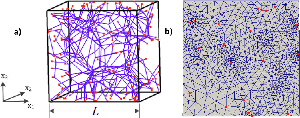
The model used in this study is shown in Fig. 1. The cubic simulation representative volume contains a network of trusses which are joined at all crossing points by freely rotating pins. These links transmit forces, but not moments. The network has additional nodes at the intersection points with the boundaries of the volume element (Fig. 1a). The entire volume is discretized using tetrahedral finite elements which are assigned matrix properties. The volume of the fibers is not explicitly represented in the model. This is not a limitation in situations, including that discussed here, in which the volume fraction occupied by fibers is small. Furthermore, the matrix prevents the fibers from coming in direct contact with each other during deformation at points other that the existing cross links, so representing the fiber volume is also not critical from this point of view.

Figure 1.

a) Schematic representation of the network. The red dots represent the points where the network intersects the model boundaries. b) Model surface showing the discretized matrix and the ends of fibers intersecting the respective plane (red dots).

The network is generated using a Voronoi procedure [12]. Seed points are placed randomly in the simulation cell and are used to construct a Voronoi tessellation. The edges of the Voronoi cells become network segments, and nodes are placed at all edge intersections and at intersections with the model boundaries. The seed points are removed after this step. Any isolated fibers or fiber clusters are removed to leave a single, fully interconnected network. Five statistically similar but distinct models were created and analyzed. Fibers are oriented isotropically inside the model. The coordination number, i.e. the number of segments emerging from each cross-link, equals four at all fiber cross-links. The network is characterized by its density, ρ, defined as the total length of fiber per unit volume, and by the mean segment length, l_c. The model size, L, (Fig. 1a)), is used to normalize all lengths in the problem. The networks analyzed in this study have densities in a narrow range bounded by 71 and 77 L⁻² which corresponds to l_c/L being 0.104. The segment lengths follow a Poisson distribution, so the entire distribution is characterized by its mean.

The solid matrix and embedded fiber network are meshed together such that mesh vertices and mesh edges on the fibers are shared with the adjacent 3D solid elements. Fig. 1(b) shows the mesh on the surface of one of the models, with the points where the fibers intersect the respective plane being marked by red dots.

Linear shape functions are used to interpolate the displacement field in both matrix and network segments. Since linear tetrahedral and truss elements have the same nodal displacement variables, compatibility between the two types of elements is ensured throughout the deformation history.

The matrix is linear elastic with Young’s modulus E_m and Poisson ratio ν_m. The fibers are described by a linear elastic model with modulus E_f, and have cross-sectional area A_f. The relevant quantity is actually the axial stiffness of the fibers, E_fA_f, which is kept as a parameter. The range over which these parameters are varied is: E_m ∈ [1, 10⁵]Pa, E_fA_f ∈ [8.17,65.34] N. This range includes the values corresponding to the collagen-agarose system studied experimentally in [11]. The results remain valid for all combinations of material parameters leading to the same non-dimensional quantities discussed in section 3.3.

The model is deformed by imposing displacement boundary conditions. A uniaxial strain is applied in the x₁ direction, ε₁₁= ε, while the faces perpendicular to the x₂ and x₃ axes are kept traction free. Most simulations are performed up to ε = 0.105 applied strain.

The overall Cauchy stress, σ̂₁₁, was evaluated based on the reactions evaluated on the face with normal in the x₁ direction, and the current area of the respective model boundary segment. Formally one may refer to stresses associated with the network and with the matrix, i.e. ${\mathrm{\sigma ̂}}_{11}={\mathrm{\sigma ̂}}_{11}^n+{\mathrm{\sigma ̂}}_{11}^m$, the two components being computed with the reactions acting at the nodes where the network intersects the model boundary and those corresponding to matrix elements, respectively. Alternatively, one may compute the two components using the strain energy stored in the matrix and network elements. However, this additive decomposition does not imply that the network and the matrix act in parallel. The central purpose of this work is to quantify the interaction between these two components.

The Newton-Raphson method was used to solve the finite element equations describing the mechanics of the coupled system. Since the constitutive behavior of all constituents is linear, the problem remains linear at small deformations. As the applied strain increases, the response becomes non-linear and the iterative procedure is used to solve the non-linear finite element equations.

3. Results

This work focuses on describing the effect of the network deformation on the matrix, and that of the matrix on the network. These effects are compared with the response of the respective isolated sub-systems, network and matrix, subjected to the same deformation. Further, the variation of the elastic moduli with system parameters is evaluated and described quantitatively using a simple mean field-type model.

3.1 Effect of the network on the matrix

The reference for this discussion is the response of the matrix to uniaxial loading. Obviously, the matrix without the embedded network deforms affinely and the stress is uniform throughout.

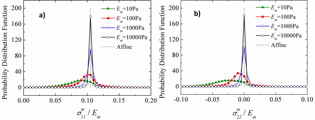
In the presence of the network, the stress in the matrix has large spatial variations. Let us consider systems in which a network with E_fA_f = 8.168 N and l_c/L = 0.104 is embedded in matrices of different moduli, E_m, and deform these systems up to ε = 0.105. Figure 2 shows the probability distribution functions (PDF) of normal stresses ${\sigma }_{11}^m$ and ${\sigma }_{22}^m$ evaluated locally in the matrix elements. ${\mathrm{\sigma ̂}}_{11}^m$ is the average of ${\sigma }_{11}^m$ over the entire matrix volume. The horizontal axis is normalized by E_m in order to allow direct comparison of the various cases considered. In the pure matrix case, the PDFs are delta functions located at 0.105 and 0 (Figs. 2a and 2b, respectively) corresponding to ${\sigma }_{11}^m$ and ${\sigma }_{11}^m$. In presence of the network, the PDFs are broad, with the second moment increasing as E_m decreases. Hence, the network induces large spatial stress variability in soft matrices. This is an important observation since the largest stress controls fracture and damage accumulation during fatigue loading.

Figure 2.

Probability distribution functions of normalized ${\sigma }_{11}^m$ (a) and ${\sigma }_{22}^m$ (b) computed in the matrix. The stress is normalized with the matrix modulus, E_m.

It is also interesting to observe that the means of the PDFs in Fig. 2a) shift to smaller values as the matrix stiffness decreases. In other words, when subjected to the same global strain, a system with a softer matrix would carry smaller normalized stresses (normalization with E_m) than a system with a stiffer matrix. A similar effect is observed in Fig. 2b) where it is seen that the mean increases in absolute value as E_m decreases. This effect was discussed in [8] and it is due to the fact that the network subjected to tension has a Poisson ratio much larger than that of the matrix. Therefore, when the same strain is imposed in the x₁ direction on the network and matrix, the network tends to shrink more in the x₂ and x₃ directions, therefore compressing the matrix. This leads to a mean compressive stress in x₂ and x₃, and, due to the Poisson effect of the matrix, to unloading in the x₁ direction.

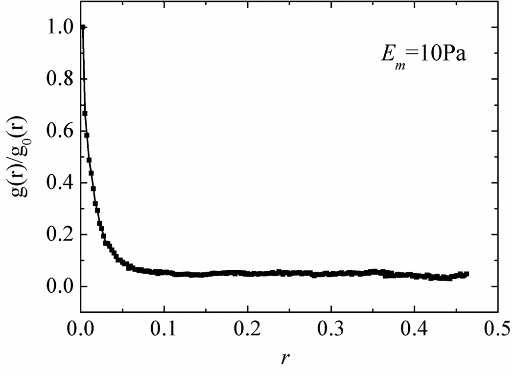
Since the fibers are represented by straight truss segments in this model, the interaction between network and matrix takes place exclusively through forces applied by the network on the matrix at the cross-links. The situation is expected to remain qualitatively similar even in presence of moderate fiber crimp and curl and when the interface between fibers and matrix are weak. This leads to significant stress concentration and a highly heterogeneous stress field characterized by the broad distributions of Fig. 2. To demonstrate the presence of such concentration sites, the locations (Gauss points) where stress is larger than a specified threshold are identified and the pair correlation function, g(r), of these points is computed. Consider a system with E_m = 10 Pa and impose a threshold equal to the standard deviation of the curve in Fig. 2a. g(r) is computed for this set of points with the origin being selected always at cross-links. The resulting function is normalized by g₀(r), the pair correlation function evaluated for all Gauss points of the matrix elements and with the same origin. The ratio g(r)/g₀(r) represents the fraction of the Gauss points carrying stresses larger than the imposed threshold (Fig. 3). It is clear that large stresses are found predominantly close to the cross-links of the network (r → 0). The asymptote at larger values of the variable represents the fraction of all Gauss points of the model carrying stresses larger than the imposed threshold.

Figure 3.

Normalized pair correlation function g(r) indicating stress concentration close to the network cross-links (i.e. at r → 0).

3.2 Effect of the matrix on the network

Networks of trusses are known to be unstable if the coordination number, z, is smaller than 2d, where d is the dimensionality of the embedding space [13]. Networks with lower coordination numbers are floppy and deform without storing energy. The networks considered in this study have coordination number z = 4, smaller than the value of 6 required for stability and hence are intrinsically floppy. As discussed in the literature [14,15,16], a floppy network can be stabilized by accounting for the bending stiffness of fibers and by transforming the cross-links into connectors that transmit both moments and forces between the fibers in contact. A floppy network acquires stiffness after a certain amount of strain is applied. In the case discussed here, the floppy network is stabilized by the presence of the matrix. Even a matrix with very small E_m would perform this function.

Fiber networks are highly heterogeneous structures which, at low density, low cross-link density, and/or low fiber bending stiffness (relative to the axial stiffness), deform non-affinely [14,17]. The deformation is approximately affine at high densities and/or higher fiber bending stiffness. Various measures of non-affinity have been proposed [14,18,19]. Here we use the measure described by:

$$H=\frac{\Vert {\mathit{u}}^{NF}-{\mathit{u}}^{AF}\Vert }{\Vert {\mathit{u}}^{AF}\Vert },$$ (1)

where u^NF and u^AF are the displacements of the cross-links in the actual case (NF), and when the deformation is affine (AF).

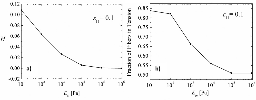
Figure 4 shows the value of the non-affinity parameter of eq. (1) computed for networks embedded in matrices with various E_m. The non-affinity is pronounced when E_m is small and decreases to zero as E_m increases. Therefore, in the limit of large matrix stiffness, the network is forced to deform affinely. This is possible only if constraint forces, the reactions of the forces acting on the matrix described in section 3.1, act on the network at the cross-links. In the limit of large E_m, the network is more compliant than the matrix and hence the internal forces imposing the compatibility of the two constituents do not lead to significant matrix deformations. Hence, in this limit, the network follows the matrix and deforms affinely.

Figure 4.

a) Variation of the nonaffinity measure of eq. (1) with the matrix elastic modulus E_m. b) Fraction of fibers loaded in tension versus the matrix modulus E_m.

This also reflects in the fraction of fibers subjected to tension. When E_m is large, the fraction is similar to that predicted by the affine model. For an effective Poisson ratio of 0.3 and affine deformation with strain ε₁₁ < 0.2, 51% of the fibers are in tension. Our model predicts an asymptote to this limit (51%) when E_m > 10⁵ Pa. For E_m=10 Pa, 84% of the fibers are in tension for all strains ε₁₁ < 0.2. When deformation is more non-affine, the amount of relaxation is larger and hence more fibers are engaged in the tensile macroscopic deformation.

3.3 Effective elastic modulus of the composite

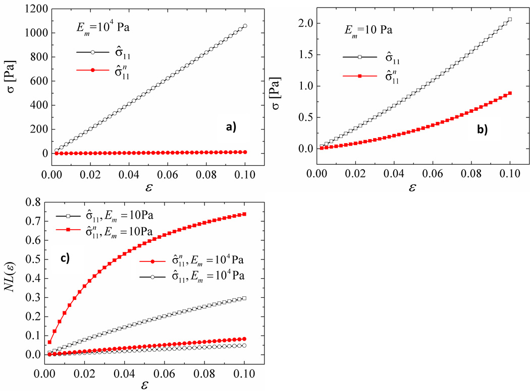
Let us analyze now the degree of non-linearity of the mechanical behavior and the effective small strain modulus of the network-matrix system. The stress-strain curves of all systems considered are non-linear. The non-linearity is purely geometric since the constitutive equations of the matrix and fiber materials are both linear. Figures 5a) and 5b) show the stress strain curves, σ̂₁₁ (ε), of two models with E_m=10 and 10⁴ Pa, respectively. The same network considered above, characterized by E_fA_f = 8.168N and l_c/L = 0.104, is embedded in the two matrices. The filled symbols correspond to the total stress σ̂₁₁ (ε), while the open symbols correspond to the component of the total stress associated with the network, ${\mathrm{\sigma ̂}}_{11}^n(\epsilon )$. In the stiffer matrix case (Fig. 5a), the network contributes little to the overall modulus, as expected, and the degree of non-linearity of σ̂₁₁ (ε) is small. The situation is reversed in the softer matrix case (Fig. 5b). The non-linearity of the network is pronounced and this reflects in σ̂₁₁ (ε). The data indicate the intuitive fact that the non-linearity in the behavior of the network-matrix system is associated with the large geometric non-linearity of the network. To make this effect more obvious, Fig. 5c) shows the contribution to these stress-strain curves from the non-linear component. Denote by Ê the small strain effective modulus of the network-matrix system (Ê = σ̂₁₁/ε for ε → 0), and further, define ${Ê}^n={\mathrm{\sigma ̂}}_{11}^n/\epsilon$ for ε → 0. The non-linear component is evaluated as

$$NL(\epsilon )=({\mathrm{\sigma ̂}}_{11}(\epsilon )-Ê\epsilon )/{\mathrm{\sigma ̂}}_{11}(\epsilon )$$ (2)

The non-linearity is much more pronounced in the soft matrix case, while the network component is always more non-linear than the total stress-strain curve.

Figure 5.

Stress-strain curves for the matrix-fiber system and for the network evaluated for systems with a) E_m = 10⁴ Pa and b) 10 Pa. c) Nonlinearity parameter of eq. (2) corresponding to the total and fiber stress-strain relationships.

Evaluating the effective modulus, Ê, and Poisson ratio, ν̂, of the network-matrix system yields additional insights. Figure 6a) shows the computed Ê function of the matrix modulus for the network considered above, with E_fA_f = 8.168N and l_c/L = 0.104 (black squares). The effective modulus is always larger than E_m and increases with increasing matrix modulus. When E_m is so large that the matrix constrains the network to deform affinely (E_m > 10⁴ Pa for this particular network), the effective modulus reaches a plateau. This plateau can be predicted by observing that in this regime both network and matrix deform affinely. Hence, the two components act as if they were in parallel in this limit. Specifically, Ê can be computed as the sum of E_m and an effective (fictitious) modulus of the affinely deforming network, $E_{aff}^n$.

Figure 6.

Variation of a) the effective modulus of the network-matrix system, Ê, and b) the effective Poisson ratio, ν̂, with the matrix stiffness E_m. The vertical axis in a) is normalized with the apparent modulus of the network constrained to deform affinely, provided by eq. (4). The prediction of the mean field model of eqs. (8) and (11) are shown by the dashed red lines in a) and b), respectively.

Let us estimate $E_{aff}^n$ by imposing an affine deformation on all network segments. For a uniaxial deformation with ε₁₁ = ε and ε₂₂ = ε₃₃ = −ν^m ε, and assuming that the fiber orientation distribution is uniform, one may write the strain energy density of an affinely deforming network as [20,21]:

$$u_{aff}^n=\frac{1}{4}\rho E_f{A}_f{\int }_0^{\pi }\text{sin}\phi {(\sqrt{{(1-{\nu }^m\epsilon )}^2\text{sin}{\phi }^2+{(1+\epsilon )}^2\text{cos}{\phi }^2}-1)}^{2}d\phi =\frac{1}{4}\rho E_f{A}_{f}F(\epsilon )$$ (3)

where φ is the angle made by the direction of given fiber with the x₁ axis and F(ε) represents the integral. Requiring that this energy density equals $1/2E_{aff}^n{\epsilon }^2$, leads to

$$E_{aff}^n=\frac{1}{2}\rho E_f{A}_{f}F(\epsilon )/{\epsilon }^2$$ (4)

Therefore, for large enough E_m, $Ê=E_m+E_{aff}^n$. $E_{aff}^n$ computed with the values of ρ and E_fA_f of this particular network is used to normalize the vertical axis in Fig. 6a). The close match with the numerical data in the plateau region provides support for the conjecture that the two components of the system act in parallel in this regime.

Figure 6b) shows the effective Poisson ratio versus E_m (black squares). As the matrix stiffness increases, the Poisson ratio decreases and becomes equal to that of the matrix, i.e. ν̂ = ν^m = 0.3. For this particular type of network, the value corresponding to E_m = 10 Pa is ν̂ = 0.376.

In order to estimate Ê for smaller values of E_m, for which the deformation is not affine, we develop a mean-field model based on the following simplified physical picture. Let us consider an isolated fiber tied to an infinite three-dimensional matrix. The system is deformed affinely by applying appropriate forces on the fiber (step 1). Note that no internal forces act on the matrix since the affine field matches the boundary conditions. The boundary of the model is then fixed and the interior is allowed to relax (step 2). In the equilibrium configuration the fiber changes length and the internal forces acting on it are the reactions of the forces acting on the matrix. Computing the energy of the system after relaxation allows evaluation of the effective stiffness of the network-matrix system based on an energetic approach similar to that used above for the affine deformation.

Two approximations are made when this approach is applied to the entire network. It is assumed that a) fibers relax independent of each other, and b) the interaction of the internal forces acting on the matrix due to fiber relaxation can be neglected.

The strain energy density of the network during the relaxation of step 2 is computed by assuming that each fiber relaxes by a fraction β of its affine deformation of step 1. Then,

$$u^n(\beta )=\frac{1}{4}\rho E_f{A}_f{(1-\beta )}^{2}F(\epsilon ).$$ (5)

The total energy stored in the matrix during the relaxation process is equal to the work performed by the internal forces. For each fiber, these are a pair of forces aligned with the fiber and acting on the matrix in opposite directions at the location of the two ends of the fiber. Under the assumption that these internal forces do not interact, the problem is equivalent to computing the work done by a force P acting on an infinite isotropic continuum, i.e. Pδ/2, where δ is the displacement of the point where P acts. Note that P is equal to the force stretching the bar and leading to the strain energy density of eq. (5). Using the Green’s function solution for an isotropic three-dimensional solid [22], one can write:

$$\frac{1}{2}P\delta =\frac{1}{2}\frac{E_m}{\alpha }{\beta }^2{L}_f^2{(\sqrt{{(1-{\nu }^m\epsilon )}^2\text{sin}{\phi }^2+{(1+\epsilon )}^2\text{cos}{\phi }^2}d\phi -1)}^2.$$ (6)

In the Green’s function solution, the energy stored in the body diverges and the solution predicts δ → ∞. To avoid this problem, an inner spherical cut-off of radius R_min needs to be taken in the vicinity of the force P. Parameter α in eq. (6) depends on ν^m and R_min as α = h(ν^m)/R_min, and hence has units of inverse length. Function h reads h(ν) = (12ν³ − 10ν² − 11ν + 11)/(24π(1 − ν)²). With this, the strain energy density stored in the matrix due to the relaxation of all (non-interacting) fibers is evaluated as:

$$u^m(\beta )=\frac{1}{4}\frac{E_m}{\alpha }\rho E_m{l}_c{\beta }^{2}F(\epsilon ).$$ (7)

Here we have taken L_f = l_c, the mean fiber length. Finding the minimum (with respect to β) of the total strain energy density u(β) = uⁿ (β) + u^m (β) leads to β = 1/(1 + η), where $\eta =\frac{E_m}{E_f}\frac{l_c}{2a{A}_f}$ is a non-dimensional parameter.

With this, one may compute the total strain energy stored and then the effective modulus of the network-matrix system, which can be written as:

$$Ê=E_m+E_{aff}^n\frac{\eta }{1+\eta }.$$ (8)

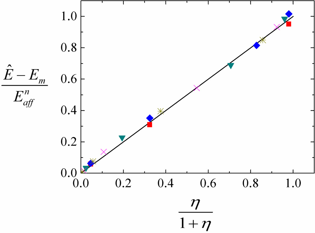
Figure 7 shows the effective modulus of the network-matrix system, (Ê −E_m) / $E_{aff}^n$, versus η/(1 + η) for several networks with different l_c/L (in the range 0.1 to 0.2) and E_fA_f (in the range 8.17 to 65.34 N) and embedded in matrices with E_m ranging from 10 to 10⁴ Pa. The same value for parameter α (i.e. α = 4/3) is used for all curves. The data collapse on the line of slope 1, providing support to eq. (8). The prediction of eq. (8) is also added to Fig. 6a) (red dashed line) and is seen to provide a good representation of the data.

Figure 7.

Variation of the normalized effective modulus of the network-matrix system with parameter η (eq. (8)) for systems with various parameters.

The effective Poisson ratio of the material can be determined using the same model. Each fiber oriented at an angle φ with respect to the loading direction acts on the matrix with a force given by (after the relaxation of step 2):

$$P_{\phi }=(1-\beta )E_f{A}_f(\sqrt{{(1-{\nu }^m\epsilon )}^2\text{sin}{\phi }^2+{(1+\epsilon )}^2\text{cos}{\phi }^2}-1),$$ (9)

which has a component in the direction perpendicular to the loading direction of magnitude P_φ sin φ. The planar density of fibers with orientation between φ and φ + dφ crossing a plane parallel to the loading direction is ρ_a = 1/2 ρ sin² φ d φ, and the effective normal stress produced by these fibers perpendicular to the loading direction can be computed as P_φ ρ_a sin φ. The average normal strain in the matrix in the x₂ direction due to the action of the network results by summing contributions of fibers with all orientations:

$${\mathrm{\epsilon ̅}}_{22}=\frac{1}{2E_m}(1-\beta )\rho E_f{A}_f{\int }_0^{\pi /2}(\sqrt{{(1-{\nu }^m\epsilon )}^2\text{sin}{\phi }^2+{(1+\epsilon )}^2\text{cos}{\phi }^2}-1){\text{sin}}^3\phi d\phi =\frac{1}{2E_m}(1-\beta )\rho E_f{A}_{f}G(\epsilon ),$$ (10)

where G (ε) represents the integral. After adding the Poisson effect of the matrix, the effective Poisson ratio can be written:

$$\mathrm{\nu ̂}={\nu }^m+{\text{lim}}_{\epsilon \to 0}|{\mathrm{\epsilon ̅}}_{22}|/\epsilon ={\nu }^m+\frac{1}{2}\frac{E_f}{E_m}\rho A_f\frac{\eta }{1+\eta }{\text{lim}}_{\epsilon \to 0}\frac{|G(\epsilon )|}{\epsilon }.$$ (11)

The prediction of eq. (11) is shown in Fig. 6b) (dashed red line) and is seen to be in good agreement with the values computed with the numerical model. The agreement is not as good at the lowest value of the matrix modulus.

It appears that, despite the approximations made, the simple model presented here captures the main features of the mechanics of this system, at least in the range of parameters considered. This indicates that, although the deformation is highly non-affine in systems with low E_m, the interaction of the internal forces is weak. Expression (8) allows for predicting the effective modulus of network composites over a broad range of system parameters.

4. Conclusions

A cross-linked fiber network embedded in an isotropic matrix introduces significant heterogeneity in the mechanics fields. The network is constrained by the matrix to deform more affinely than it would in the absence of the embedding medium. This occurs due to internal forces applied by the matrix on the network. The reactions of these forces act on the matrix and introduce significantly heterogeneous stress and strain fields which are concentrated around the network cross-links. Hence, damage is expected to nucleate at these concentration sites. The network also renders the deformation of the network-matrix ensemble non-linear, the degree of non-linearity depending on the stiffness of the matrix, i.e. on the degree of network constraint. The effective small-strain modulus of the composite can be captured with a simple micromechanics model in terms of system parameters.

References

- 1.Algar WH. Effect of structure on the mechanical properties of paper. In: Bolam F, editor. Consolidation of the Paper Web. 1965. pp. 814–849. [Google Scholar]
- 2.Jeffery AK, Blunn GW, Archer CW, Bentley G. J. Bone Joint Surg. 1991;73:795. doi: 10.1302/0301-620X.73B5.1894669. [DOI] [PubMed] [Google Scholar]
- 3.Mofrad MRK. Cytoskeletal mechanics: models and measurements. Cambridge University Press; 2006. [Google Scholar]
- 4.Rigdahl M, Hollmark H. Network mechanics. In: Bristow JA, Koleth P, Marcel Dekker, editors. Paper structure and properties. Ch. 12. 1986. p. 241. [Google Scholar]
- 5.Astrom J, Saarinen S, Niskanen K, Kurkijarvi J. J. Appl. Phys. 1994;75:2383. [Google Scholar]
- 6.Cortes DH, Elliott DM. Biomech. Model. Mechanobiol. 2012;11:781. doi: 10.1007/s10237-011-0351-x. [DOI] [PMC free article] [PubMed] [Google Scholar]
- 7.Lake SP, Hadi MF, Lai VK, Barocas VH. Ann. Biomed. Eng. 2012;40:2111. doi: 10.1007/s10439-012-0584-6. [DOI] [PMC free article] [PubMed] [Google Scholar]
- 8.Zhang L, Lake SP, Lai VK, Picu RC, Barocas VH, Shephard MS. J. Biomech. Eng. 2013;135 doi: 10.1115/1.4023136. 011008(1–9). [DOI] [PMC free article] [PubMed] [Google Scholar]
- 9.Peng XQ, Guo ZY, Moran B. J. Appl. Mech. 2006;73:815. [Google Scholar]
- 10.O'Connell GD, Guerin HL, Elliott DM. J Biomech Eng. 2009;131:111007. doi: 10.1115/1.3212104. [DOI] [PMC free article] [PubMed] [Google Scholar]
- 11.Lake SP, Barocas VH. Ann. Biomed. Eng. 2011;39:1891. doi: 10.1007/s10439-011-0298-1. [DOI] [PMC free article] [PubMed] [Google Scholar]
- 12.Nachtrab S, Kapfer SC, Arns CH, Madadi M, Mecke K, Schroder-Turk GE. Adv. Mater. 2011;23:2633. doi: 10.1002/adma.201004094. [DOI] [PubMed] [Google Scholar]
- 13.Kellomäki M, Åström J, Timonen J. Phys. Rev. Lett. 1996;77:2730. doi: 10.1103/PhysRevLett.77.2730. [DOI] [PubMed] [Google Scholar]
- 14.Head DA, Levine AJ, MacKintosh FC. Phys. Rev. E. 2003;68:061907. doi: 10.1103/PhysRevE.68.061907. [DOI] [PubMed] [Google Scholar]
- 15.Shahsavari A, Picu RC. Phys. Rev. E. 2012;86:011923. doi: 10.1103/PhysRevE.86.011923. [DOI] [PubMed] [Google Scholar]
- 16.Picu RC. Soft Matter. 2011;7:6768. [Google Scholar]
- 17.Chandran PL, Barocas VH. J. Biomech. Eng. 2006;128:259. doi: 10.1115/1.2165699. [DOI] [PubMed] [Google Scholar]
- 18.Onck PR, Koeman T, Van Dillen TT, van der Giessen E. Phys. Rev. Lett. 2005;95:178102. doi: 10.1103/PhysRevLett.95.178102. [DOI] [PubMed] [Google Scholar]
- 19.Hatami-Marbini H, Picu RC. Phys. Rev. E. 2008;77:062103. doi: 10.1103/PhysRevE.77.062103. [DOI] [PubMed] [Google Scholar]
- 20.Lee DH, Carnaby GA. Textile Res. J. 1992;62:185. [Google Scholar]
- 21.Wu XF, Dzenis YA. J. Appl. Phys. 2005;98:093501. [Google Scholar]
- 22.Love AEH. A treatise on the mathematical theory of elasticity. Dover Pub.; 1944. [Google Scholar]