Novel Hybrid GPU–CPU Implementation of Parallelized Monte Carlo Parametric Expectation Maximization Estimation Method for Population Pharmacokinetic Data Analysis

Abstract

The development of a population PK/PD model, an essential component for model-based drug development, is both time- and labor-intensive. A graphical-processing unit (GPU) computing technology has been proposed and used to accelerate many scientific computations. The objective of this study was to develop a hybrid GPU–CPU implementation of parallelized Monte Carlo parametric expectation maximization (MCPEM) estimation algorithm for population PK data analysis. A hybrid GPU–CPU implementation of the MCPEM algorithm (MCPEM_GPU) and identical algorithm that is designed for the single CPU (MCPEM_CPU) were developed using MATLAB in a single computer equipped with dual Xeon 6-Core E5690 CPU and a NVIDIA Tesla C2070 GPU parallel computing card that contained 448 stream processors. Two different PK models with rich/sparse sampling design schemes were used to simulate population data in assessing the performance of MCPEM_CPU and MCPEM_GPU. Results were analyzed by comparing the parameter estimation and model computation times. Speedup factor was used to assess the relative benefit of parallelized MCPEM_GPU over MCPEM_CPU in shortening model computation time. The MCPEM_GPU consistently achieved shorter computation time than the MCPEM_CPU and can offer more than 48-fold speedup using a single GPU card. The novel hybrid GPU–CPU implementation of parallelized MCPEM algorithm developed in this study holds a great promise in serving as the core for the next-generation of modeling software for population PK/PD analysis.

INTRODUCTION

Population pharmacokinetics (PK) and pharmacodynamics (PD) model development is an important step in the model-based drug development approach that can increase the efficiency of drug development. The developed population PK/PD model allows for the integration of PK and PD information into the drug development plan and has the potential to accelerate the evaluation of drugs in humans (1,2). Currently, most population PK/PD models have been developed using the nonlinear mixed-effect (NLME) method. However, the population parameters estimated from the most commonly used first-order (FO), first-order conditional method (FOCE), and Laplacian method (LAP) in NONMEM, a standard population PK/PD data analysis program, are based on model approximation and not true maximum likelihood estimators. Therefore, the statistical properties of maximum likelihood estimators such as the standard error derived from the Fisher information matrix, or the likelihood ratio test for nested models, do not hold for these methods although they are commonly applied in practice for the analysis of population PK/PD data (3–6). In recent years, a series of new NLME estimation methods have been developed for population PK/PD modeling. Most notably are the expectation maximization (EM) methods based on exact likelihood functions such as the Monte Carlo parametric expectation maximization (MCPEM) method that developed by Walker and Schumitzky (7,8) and implemented in S-ADAPT (5,6), and the stochastic approximation of expectation maximization (SAEM) methods that first proposed and used in MONOLIX (3). Because of the absence of linear approximation in these methods, the parameters obtained from MCPEM and SAEM are true maximum likelihood estimates for which all the statistical properties of maximum likelihood can be applied (6). Both of these methods offer an opportunity to match the sophisticated needs of drug development with state-of-the-art methodology and hold a great promise in serving as the core for the next generation of NLME-modeling software tools for population PK/PD analysis.

Despite the advancement of the NLME methodologies, the development of the population PK/PD model for drug development remains a very time- and labor-intensive process. With the increased model complexity and amount of data processed used in the analysis; population PK/PD model development time is now limiting the impact of the model- and evidence-based drug development approach. Until now, two different approaches have been proposed to improve the efficiency of population PK/PD model development by implementing the NLME estimation method in a highly parallelized supercomputer or distributed computing cluster (9–11). However, the most relevant limitation of these approaches is represented by its cost: supercomputers and distributed computing cluster are very expensive. A total 5-year life cycle cost for operating a Cray X1 supercomputer and a distributed computing cluster with a comparable performance is about 54 million US dollars in 2003 (12). In addition, these machines are not energy-efficient and require significant resources to power and cool down the system.

Recently, a graphical-processing unit (GPU) has been proposed and used to accelerate the scientific computation in many fields including quantum mechanics, medical imaging, and video/audio processing (13). GPU is a dedicated numerical processor originally designed for rendering complex three-dimensional computer graphics. Compared to a standard central processing unit (CPU), current GPUs have hundreds of numerical processor cores on a single chip and can be programmed to perform many numerical operations simultaneously to achieve extremely high arithmetic intensity for complex numerical analysis. Currently, one of the world’s fastest and most power-efficient supercomputers installed at Oak Ridge National Laboratory which can achieve 17.59 Petaflop/s (quadrillions of calculations per second), is powered by GPU-computing technology (14). Furthermore, the GPU is considered to be one of the more energy-efficient architectures compared to standard CPU computing platform (15). These unique features make it feasible to implement the state-of-the-art NLME analytical approaches using a low-cost and relatively energy-efficient GPU parallel computing platform. This can substantially decrease the time required to construct a complex population PK/PD models for model-based drug development. MCPEM is a Monte Carlo EM method where the analytically intractable expectation (E)-step of EM algorithm is computed numerically through Monte Carlo simulation using sampling techniques, and it has been used successfully in developing complex population PK/PD model (16). One of the unique features of the MCPEM is that the E-step of calculating a conditional mean and variance of individual subjects needed to update the population PK/PD parameters in the maximization (M)-step can be estimated independently (5,7). This important characteristic makes MCPEM an ideal NLME method that can take full advantage of the GPU-based parallel computing power to improve the efficiency of complex population PK/PD model development.

The objectives of the present study were to (1) highlight the methodology of first hybrid GPU–CPU implementation of MCPEM method and (2) to compare the performance of this novel hybrid CPU-MCPEM method in population pharmacokinetic data analysis.

METHOD

MCPEM and Computing Platform

Data were analyzed by the nonlinear mixed-effects modeling method utilizing the MCPEM algorithm. The theory and detail implementation of the MCPEM algorithm have been described in detail previously (5–7,16). Briefly, in the MCPEM algorithm, likelihood is maximized with respect to the population mean (μ) and variance (Ω) by first evaluating the conditional mean and conditional variance for each subject using fixed values of μ and variance Ω during the expectation step E according to Eqs. (1) and (2), and then followed by evaluating updates to μ and Ω using Eqs. (3) and (4) (the maximization step M) (5,7).

Expectation (E) Step:

1

2

Maximization (M) Step:

3

4

Where p(y_i,θ|μ,Ω) is the joint likelihood function. The E and M steps were repeated until μ and Ω no longer change. At this point, exact marginal density is maximized and the final population parameters μ and Ω that best describes the data were obtained (5,7). For MCPEM algorithm developed in this study, the Monte Carlo integration method with direct sampling is used to evaluate and during the expectation step (5). The intra-individual variance was updated according to Vapprox = 3 method in S-ADAPT program (17).

The flow chart of the hybrid GPU–CPU implementation of the MCPEM algorithm (MCPEM_GPU) is shown in Figure 1 and the detail steps are summarized as follow:

1. Program initialization

2. Begin iteration loop from iteration 1 to maximum assigned iteration number

3. For a given iteration, the CPU transfer the observed concentration/dosing data of individual subject and generated random model parameters sets for E calculation to GPU processing card

4. The likelihoods p(y_i,θ|μ,Ω) (in Eq. 1) for each generated random model parameter set θ within an assigned subject are evaluated simultaneously in parallel fashion by the processes cores on the GPU and the results are stored in the local GPU memory

5. After likelihoods p(y_i,θ|μ,Ω) for all generated random model parameter set θ are obtained, these results are transferred back to CPU and used to compute the conditional means and variances of each subjects according to Eqs. 1 and 2 in the E-steps of the EM algorithm. Repeat steps 2 and 5 until conditional mean and and variance are computed for all subjects.

6. The CPU executes the M step according to Eqs. (3) and (4) using the E-step results of all subjects

7. Repeat steps 2 to 6 until the maximum iteration number is reached.

Fig. 1.

Flow chart of MCPEM_GPU algorithm in heterogeneous GPU–CPU computing platform. Boxes highlighted in gray computation within GPU processor cores

To evaluate the performance of the MCPEM_GPU algorithm developed in this study, an identical MCPEM program that performs the complete analysis on a single CPU (MCPEM_CPU) was developed and generated the results for comparison purposes. Furthermore, parallelized MCPEM algorithm implemented in the NONMEM (MCPEM_NONMEM) with similar settings was used as an external reference to assess the model computation times of MCPEM_GPU. Both MCPEM_GPU and MCPEM_CPU algorithms were developed in a computer equipped with 64-bit Windows 7 (Microsoft Corporation, Redmond, WA), 6-core Xeon X5690 CPU (Intel Corporation, Santa Clara, CA) and a Tesla C2070 parallel computing GPU card (NVIDIA, Santa Clara, CA) that contains 448 numerical processor cores and 6 GB onboard SDRAM memory. The MCPEM algorithm was written in MATLAB (2009a, The MathWorks, Natick, MA). In addition, JACKET ® GPU toolbox for MATLAB (1.7, AccelerEyes, Atlanta, GA) and NVIDIA CUDA GPU-computing toolbox (3.2, Santa Clara, CA) were used to develop GPU section of the MCPEM_GPU algorithm. Parallelized MCPEM_NONMEM was executed in 10 CPU cores of Intel Xeon X5690 CPU at a clock speed of 3.46 GHz using File Passing Interface method with the following settings: METHOD = DIRECT INTERACTION CTYPE = 0 SEED = 12345 ITER = 30. The number of Monte Carlo random sample (ISAMPLE) used was identical to those in MCPEM_GPU and MCPEM_CPU.

Data

Two simulated model/sampling design scenarios were used for the analysis. The first model/sampling design scenario is a one-compartment PK model with linear elimination process and intensive PK sampling design. The model parameters include the systemic clearance (CL) and the volume of distribution (V_c). Model parameters were randomly selected from a log-normal multivariate distribution with variances ω²_CL and ω²_Vc, and off-diagonal elements (covariances) were set to zero. Residual variability of the observed concentrations was described by a proportional error model with a variance parameter (σ²). Therefore, a total of five population parameters were used to describe this PK model: CL, V, ω²_CL, ω²_Vc, and σ². Population parameters used to simulate the data for analysis are as follow: CL = 0.1 L/h, V = 1 L, ω²_CL = ω²_Vc = 0.1, and σ² = 0.1. In order to compare the performance of the MCPEM without the burden of sparse incomplete design in this example, we chose to simulate the data using intensive sampling design that provided sufficient information for the parameter estimations. PK samples were simulated at 0.5, 1, 2, 4, 6, 8, 12, 24, and 48 h after a single IV bolus dose of 100 units. Furthermore, the initial parameters used for model analysis were set close to the true population parameters in order to avoid possible trapping of EM algorithm in local minimum and are shown as follow: CL = 0.2 L/h, V = 2 L, ω²_CL = ω²_Vc = 0.3, and σ² = 0.1.

The second model/sampling design scenario is two-compartment linear PK model with two data points per subjects. This is the similar model that used in our early study to determine parameter assessment of different NLME methods in a sparse data sampling design (6). The model parameters consist of CL, V_c, distribution clearance (Q), and volume of distribution for the peripheral compartment (V_p). Inter-individual variability (ω²_CL, ω²_Vc,ω²_Q, ω²_Vp) was described by log-normal distribution and there was no correlation between the model parameters, and proportional error model with a variance parameter (σ²) was used to describe the residual variability. Population parameters used to simulate the data for analysis are as follow: CL = 5.0 L/h, V_c = 5.0 L, Q = 2.0 L/h, V_p = 10 L, ω²_CL = 0.1, ω²_Vc = 0.1, ω²_Q = 0.1, ω²_Vp = 0.1, and σ² = 0.1. For each subject, simulations were performed with an intravenous bolus dose of 1000 unites and data with residual error were simulated at two sampling times from a discrete set of times: 0.1, 0.2, 0.4, 0.7, 1, 2, 4, 7, 10, 20, 40, and 70 times units after drug administration. All possible pairs of times with 66 different combinations were equally represented among the subjects in each simulated trial. This balanced sampling design was expected to provide sufficient information to obtain both inter-subject and residual variability despite the sparse amount of data per subject (6). The following initial parameters were used for model analysis: CL = 3.0 L/h, V_c = 3.0 L, Q = 3.0 L/h, V_p = 10 L, ω²_CL = 0.3, ω²_V1 = 0.3, ω²_Q = 0.3, ω²_V2 = 0.3, and σ² = 0.1.

A MATLAB script was written to drive in batch mode for all model estimation processes. Results were automatically processed in MATLAB. Bias of the parameter estimation from different estimation methods was evaluated by percent relative estimation error (RER) (18):

5

where θ_k were parameter estimations, and θ_ktrue were “true” values of parameters for individual kth simulated trial. θ_ktrue for population mean and variance was obtained by computing the mean and variance for the log simulated individual PK parameters for kth simulated trial. θ_ktrue for σ² = 0.1 which was the true value used for data simulation. A boxplot was chosen to visually represent and compare the values of RER. In addition, a mean percent RER (MRER) value was determined using the following equation:

6

where θ_k and θ_ktrue represented estimated and “true” values of parameters from kth simulated trial, respectively. K is the total number of simulated trials used to calculate the MRER which is 100 in this analysis.

Precision of the parameter estimation were evaluated using mean percent absolute relative estimation error (MARER):

7

During preliminary analysis, the population parameters achieved consistent stability between 20–30 EM iterations. Hence, the model computation time was defined as the time for the MCPEM algorithm to complete 30 EM iterations and population parameters obtained from the last iteration was used as the final population parameter estimates. In order to compare the computation times of different algorithms, times to complete the model analysis were recorded automatically using MATLAB script function. In addition, a speedup factor (SF) is used to compare the performance of the parallelized MCPEM_GPU algorithm with the MCPEM_CPU executed in a single CPU (19):

8

To compare the effects of different number of random Monte Carlo model parameters (N_MC) used to compute the MCPEM E-steps on the performance of MCPEM_GPU, the computation times and SF were assessed using 500, 1,000, 2,000, 5,000, 10,000, and 20,000 random Monte Carlo model parameters. In addition, different numbers of subjects (N_SUB) of 50, 100, 200, and 500 were simulated in each trial for first model/sampling design scenario and used to determine the effect of subject number on MCPEM_GPU performance. In a second model/sampling design scenario, different N_SUB of 200, 500, and 1,000 were simulated for each individual trial.

RESULTS

For the first model/sampling design scenario with one-compartment linear PK and rich sampling design, both MCPEM_CPU and MCPEM_GPU algorithm produced identical model parameter estimates regardless of the number of Monte Carlo model parameters sets (N_MC) used for E-Step computation. Bias of the parameter estimations for both algorithms was shown in Fig, 2a and Table I. Using N_MC of 1,000 in E-step computation, the MRER was 0.024, 0.011, −3.3, −2.5, and 0.54 for CL, V_c, ω²_CL, ω²_Vc, and σ², respectively, for both MCPEM_CPU and MPCEM_GPU algorithms. When the N_MC of 10000 was used for E-Step computation, the MRER was 0.14, −0.084, −2.4, −1.9, and 0.37 for CL, V_c, ω²_CL, ω²_Vc, and σ², respectively. These results suggested that both MCPEM_CPU and MCPEM_GPU algorithm produced a relatively small bias (less than ±10% of MERER) in parameter estimation. Precision of model parameters estimation measured by MARER calculation was shown in Table I. For N_MC of 1000, the MARER was 0.92, 1.1, 5.9, 6.7 and 2.6 for CL, V_c, ω²_CL, ω²_Vc, and σ², respectively for both MCPEM_CPU and MCPEM_GPU algorithms. The MARER was 0.94, 1.0, 5.6, 6.2 and 2.2 for CL, V_c, ω²_CL, ω²_Vc, and σ², respectively, if N_MC of 10,000 was used to compute E-Step of MCPEM algorithm.

Fig. 2.

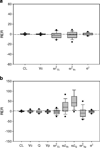
Box plots of percent relative estimation error (RER) for model parameters in MCPEM_GPU for a first and b second model/sampling design scenario. CL clearance; V _c volume of distribution at central compartment; Q distribution clearance; V _p volume of distribution at peripheral compartment; ω ² _CL population variance of CL; ω ² _Vc population variance of V _c; ω ² _Q population variance of Q; ω ² _Vp population variance of Vp; σ ² variance of intra-individual proportional error model. N _MC = 10000; N _SUB = 100. Both MCPEM_GPU and MCPEM_CPU produced identical results

Table I.

Bias (MRER) and Precision (MARER) of Estimated Fixed and Random Effects of MCPEM_GPU and MCPEM_CPU. For the First Model/Sampling Design Scenario: One-Compartment Linear PK Model with Rich Sampling Design

Methods	CL	V c	ω 2 CL	ω 2 Vc	σ 2
MRERa
N MC = 1000	0.024	0.011	−3.3	−2.5	0.54
N MC = 1000	0.14	−0.084	−2.4	−1.9	0.37
MARERa
N MC = 1000	0.92	1.1	5.9	6.7	2.6
N MC = 10000	0.94	1.0	5.6	6.2	2.2

MRER mean percent relative estimation error; MARER mean percent absolute relative estimation error. Total number of simulation trial used for MRER/MARER calculation = 100; number of subject for each simulation trial = 100; N _MC the number of Monte Carlo parameters set used to compute the E-step of the MCPEM algorithm; CL population (typical) clearance; V _c population (typical) distribution volume at central compartment; ω ² _CL population variance of CL; ω ² _Vc population variance of V _c; σ ² variance of intra-individual proportional error model

^aBoth MCPEM_GPU and MCPEM_CPU produced identical results

The model computation times of MCPEM_GPU were consistently shorter than the MCPEM_CPU. Using N_MC of 1,000 and 100 subjects in each simulated trial, the mean (range) computation times of MCPEM_GPU and MCPEM_CPU were 0.156 (0.149–0.161) and 1.25 (1.23–1.28) min, respectively. The mean (range) computation times of MCPEM_NONMEM were 0.366 (0.317–0.479). The mean computation times to obtain the population parameter estimates from 100 simulated trials with 100 subjects per trial for MCPEM_GPU were 0.147, 0.156, 0.176, 0.224, 0.336, and 0.531 min for N_MC of 500, 1,000, 2,000, 5,000, 10,000, and 20,000, respectively (Fig. 3a). The mean computation times for MCPEM_CPU were 0.621, 1.25, 2.49, 6.18, 13.0, and 25.7 min for N_MC of 500, 1,000, 2,000, 5,000, 10,000, and 20,000, respectively (Fig. 3a). The corresponding mean SF values were 4.23, 8.01, 14.3, 27.7, 38.8, and 48.4 (Fig. 3a). The mean computation times for MCPEM_NOMEM were 0.274, 0.366, 0.494, 0.939, 1.57, and 2.91 min for N_MC of 500, 1,000, 2,000, 5,000, 10,000, and 20,000, respectively. Result for mean model computation times of simulated trial with different number of subjects (N_SUB) is presented in Fig. 3b. Again, the model computation times of MCPEM_GPU were consistently shorter than the MCPEM_CPU. The mean model computation times of MCPEM_GPU with N_MC of 1000 were 0.156, 0.311, and 0.776 min for N_SUB of 100, 200, and 500, respectively. These compared to the mean computation times of MCPEM_CPU of 1.25, 2.48, and 6.23 min. The corresponding mean SF values were 8.01, 7.96, and 8.03 (Fig. 3b). The mean computation times of MCPEM_NOMEM were 0.366, 0.501, and 0.776 min for N_SUB of 100, 200, and 500, respectively.

Fig. 3.

a The relationships between mean model computation time of the MCPEM_CPU, MCPEM_GPU and MCPEM_NONMEM, and speedup factor of MCPEM_GPU with N _MC for first model/sampling design scenario. N _SUB = 100; Number of simulated trials = 100. b The relationships between mean model computation time of the MCPEM_CPU, MCPEM_GPU, and MCPEM_NONMEM, and speedup factor of MCPEM_GPU with N _SUB. N _MC = 1000; Number of simulated trials = 100. Closed circle MCPEM_CPU; closed square MCPEM_GPU; closed triangle MCPEM_NONMEM; open circle speedup factor (SF)

For the second model/sampling design scenario with two-compartment linear PK and sparse sampling design, bias and precision of the parameter estimations of MCPEM_GPU and MCPEM_CPU were shown in Fig. 2b and Table II, and both algorithms produced identical model parameter estimates. For N_MC of 1,000 and 10,000, both MCPEM_CPU and MCPEM_GPU algorithm produced a relatively small bias (less than ±10% of MRER) for most parameter estimation except for ω²_Vc and ω²_Q. The relatively large values of MRER for ω²_Vc and ω²_Q were probably due to both sparse sampling design and relatively small number of subjects (N_SUB = 200) used to obtain the parameter estimation.

Table II.

Bias (MRER) and Precision (MARER) of Estimated Fixed and Random Effects for the Second Model/Sampling Design Scenario: Two-Compartment Linear PK Model with Sparse Sampling Design

Methods	CL	V c	Q	Vp	ω 2 CL	ω 2 Vc	ω 2 Q	ω 2 Vp	σ 2
MRERa
N MC = 1000	−0.89	−1.1	−1.0	−1.1	−4.8	11	50	−12	−0.81
N MC = 10000	−0.65	−0.15	−1.8	−1.5	−4.0	22	52	−6.7	−2.5
MARERa
N MC = 1000	2.0	3.7	6.0	4.7	12	22	53	21	5.7
N MC = 10000	1.9	4.5	4.2	4.2	12	30	54	23	5.4

MRER mean percent relative estimation error; MARER mean percent absolute relative estimation error. Total number of simulation trial used for MRER/MARER calculation = 100; number of subject for each simulation trial = 200; N _MC the number of Monte Carlo parameters set used to compute the E-step of the MCPEM algorithm; CL population (typical) clearance; V _c population (typical) distribution volume at central compartment; ω ² _CL population variance of CL; ω ² _Vc population variance of V _c; σ ² variance of intra-individual proportional error model

^aBoth MCPEM_GPU and MCPEM_CPU produced identical results

Using N_MC of 1,000 and 200 subjects in each simulated trial, the mean (range) computation times of MCPEM_GPU and MCPEM_CPU were 0.392 (0.379–0.416) and 2.42 (2.38–2.47) min, respectively. The mean (range) computation times of MCPEM_NONMEM were 0.254 (0.237–0.310). The mean computation times to obtain the population parameter estimates from 100 simulated trials with 200 subjects per trial for MCPEM_GPU were 0.366, 0.392, 0.440, 0.623, 0.817, and 1.15 min for N_MC of 500, 1,000, 2,000, 5,000, 10,000, and 20,000, respectively (Fig. 4a). The mean computation times for MCPEM_CPU were 1.20, 2.42, 4.65, 12.6, 25.1, and 50.7 min. The corresponding mean SF values were 3.27, 6.17, 10.6, 20.0, 30.8, and 44.1. The mean computation times for MCPEM_NONMEM were 0.229, 0.254, 0.315, 0.496, 0.767, and 1.30 min for N_MC of 500, 1,000, 2,000, 5,000, 10,000, and 20,000, respectively. The relationships between mean model computation times of simulated trial with different number of subjects (N_SUB) are shown in Fig. 4b. The computation times for MCPEM_GPU were consistently shorter than the MCPEM_CPU regardless of number of subject in simulated trial. The mean model computation times of MCPEM_GPU with N_MC of 1000 were 0.391, 0.967, and 1.95 min, compared with MCPEM_CPU of 2.42, 5.81, and 11.6 min for N_SUB of 200, 500, and 1000, respectively. The corresponding mean SF values were 6.17, 6.00, and 5.98. The mean computation times of MCPEM_NOMEM were 0.254, 0.361, and 0.514 min for N_SUB of 200, 500, and 1000, respectively.

Fig. 4.

a The relationships between mean model computation time of the MCPEM_CPU, MCPEM_GPU, and MCPEM_NONMEM and speedup factor of MCPEM_GPU with N _MC for second model/sampling design scenario. N _SUB = 100; Number of simulated trials = 100. b The relationships between mean model computation time of the MCPEM_CPU, MCPEM_GPU, and MCPEM_NONMEM, and speedup factor of MCPEM_GPU with N _SUB. N _MC = 1,000; Number of simulated trials = 100. Closed circle MCPEM_CPU; closed square MCPEM_GPU; closed triangle MCPEM_NONMEM; open circle speedup factor (SF)

DISCUSSIONS

In this study, the objective was to develop a fast and efficient hybrid GPU–CPU implementation of parallelized MCPEM method (MCPEM_GPU) for analyzing population pharmacokinetic data. Executed with a single GPU card, the developed MCPEM_GPU method can offer more than 48-fold speedup and yields identical parameter estimations compared to a CPU-based method that contains analogous serial code (MCPEM_CPU). Therefore, we believe that our objective was achieved. In addition, this article is the first published report to describe the detail hybrid GPU–CPU implementation of parallelized MCPEM algorithm for population data analysis.

Several linear approximation NLME methods such as FO and FOCE method has been used in population PK/PD analysis (20) but these methods may contain considerable errors if the statistical assumptions of these methods were violated (3–5). This has motivated the use of the method that can estimate the exact likelihood function, specifically, the Monte Carlo EM algorithm such as MCPEM and SAEM (3, 5, 7, 8). These exact EM methods has been shown to have great stability in analyzing simple or complex population PK/PD data and can provide accurate results with sparse or rich data (6, 21, 22). Traditionally, the population models were developed using these NLME algorithms implemented on a single computer platform, e.g., the population parameters were obtained by analyzing all the individual subjects sequentially from the population in a single computer. Due to the model complexity and number of analyzed subjects in the population, model development using this approach can be very time and resource intensive.

Recent advances in GPU-computing technology make it possible to build an energy-efficient and high power parallel computing platform for developing a population PK/PD model for drug development. GPU is a stream processor that can only process independent data elements from data record, but can process many of them in parallel. A stream is a set of data records that require similar computation. In this sense, the GPU computing is optimized for “data parallelism” and is effectively executed only if numerical computation can be operate in parallel by running the same function (kernel) to each elements of a dataset simultaneously on multiple cores of the GPU. Therefore, not all numerical methods and problems can be effectively solved with GPU-computing technology. For this reason, the distributed computing approach implemented in standard population PK/PD analysis software such as NONMEM and S-ADAPT which assigned individual subject to different computing node cannot be used in current GPU-computing environment because the early termination of the computation in any subjects (due to differences in number of observation and dosing history) will cause the premature termination of the computation for the remaining subjects in other GPU cores. Among the available NLME algorithms, MCPEM is especially well-suited for GPU-computing because the same kernel function can be used to compute joint likelihood p(y_i,θ|μ,Ω) for each of many simulated Monte Carlo random model parameters sets θ during the E-step in order to obtain conditional mean θ_i and variance B_i for individual subjects.

The method described in this study was specifically designed to utilize the power of GPU-computing technology for analyzing population data with MCPEM algorithm. In the early phase of development, the computational times of all analysis steps were assessed and evaluated for the feasibility of implementing the program code in a GPU-computing platform. The joint likelihood calculation for each generated random model parameter set within an assigned subject during the E-step of MCPEM algorithm was identified as the most computationally intensive and rate-limiting step of the MCPEM algorithm because this calculation has to be performed many times for each subjects and can be analyzed separately and implemented effectively in GPU-computing environment. Consequently, we focused on parallelizing this step on the GPU in order to improve the computing efficiency of the MCPEM method. Because the MCPEM_GPU implemented in this study is parallelized within an individual subjects and not among subjects in the population, the computational times of the MCPEM_GPU, similar to those observed with MCPEM_CPU, was expected to be increased in a linear fashion as the number of subjects in the dataset was increased. Therefore, the SF remained constant and did not change with number of subjects included in the analysis.

The Compute Unified Device Architecture (CUDA) is an application programming interface (API) developed by NVIDIA (Santa Clara, CA) for general-purpose computing on CUDA-compatible NVIDIA graphics processor card. The development of CUDA allows scientific researchers to take advantage of GPU’s parallel computing power without using any specific graphics APIs (23). The GPU-computing features described in this study were implemented in MATLAB using Jacket, a software toolbox which translates MATLAB code into CUDA-compatible code that runs on CUDA-enabled GPUs. The parallel analysis steps in this study utilized the GFOR loop construct implemented in Jacket to simultaneously launch and perform the joint likelihood calculation for many generated random model parameter sets within the subject on the GPU (24). The combination of MATLAB and Jacket is convenient because it allows scientific researchers to rapidly develop prototype programs for GPU-accelerated data analysis using a familiar, high-level language (MATLAB). While the MATLAB script of our GPU-based method performs well compared to CPU methods, greater time performance improvement may be achieved by using a lower-level GPU-computing platform (e.g., C for CUDA) to implement the method. Also, while the results shown in our study were obtained using only a single GPU card, it is expected that developed MCPEM_GPU algorithm can be even more efficient in a multiGPU-computing environment. Further study is ongoing to assess the performance improvement of the MCPEM_GPU algorithm can achieve using multiple GPU cards.

In an ideal parallel computing situation, one would expect the time performance difference between calculating likelihoods of many generated random model parameters set (N_MC > 500) in parallel and analyzing them in serial to be much greater than the 48-fold difference observed in this study. However, there are several factors limiting the time improvement that could achieve with GPU parallelization. First, the clock speeds of the Xeon X5690 CPU and Tesla C2070 GPU cards used for our analyses are 3.46 GHz and 0.575 GHz, respectively. Thus, a CPU processor core could execute a computation step much faster than a GPU processor. In addition, the developed MCPEM_GPU algorithm cannot calculate the likelihood from more than 448 generated random model parameter sets at one time due to the limited number of processor cores in a Tesla C2070 GPU card. Furthermore, several computation steps including the calculation of conditional variance for each subject during the E-step of MCPEM cannot be implemented in GPU-computing platform easily without major code modification and has to compute with CPU using a standard serial code, and this limit the ability of MCPEM_GPU to achieve higher SF value. Lastly, it is possible that the necessary memory transfers to and from the GPU card in MCPEM_GPU algorithm would also generate additional time costs compared to a CPU-based method. However, the parallelized steps of our MCPEM_GPU algorithm occurred within the same subjects and only the simulated Monte Carlo parameters and its corresponding joint likelihood estimation were transferred between CPU and GPU. In addition, only the data from a single subject was transferred and stored in the GPU memory at a time. Given that the data transfer between GPU and CPU is direct and extremely fast with the rate of about 5 GT/s with Tesla C2070 card used in this study, therefore, it is unlikely that the data transfer between CPU and GPU was the major contributing factor for observed SF in this study.

Due to different programming languages (FORTRAN in NONMEM/S-ADAPT and MATLAB/C++ for MCPEM_GPU) and other factors such as variation of random number generators and other numerical methods used for developing the MCPEM algorithms, it was very difficult to directly compare the model computation times and obtain the meaningful SF of our MCPEM_GPU with parallelized MCPEM in NONMEM/S-ADAPT. Nevertheless, the parallelized MCPEM algorithm in NONMEM (MCPEM_NONMEM) was useful to serve as an external reference in assessing the general performance of MCPEM_GPU for population data analysis. The MCPEM_NONMEM using 10 CPU cores of Intel Xeon CPU X5690 CPU at clock speed of 3.46 GHz achieved comparable model computation times with MCPEM_GPU which ran on 448-cores GPU-computing card with 0.575 GHz clock speed. The possible reason of this finding was that the FORTRAN-based MCPEM_NONMEM offered much faster numerical computation than the MCPEM_GPU which mainly developed with slower MATLAB programming language, and therefore, able to achieve comparable model computation times while ran on less number but faster CPU cores.

To our best knowledge, the compatible ordinary differential equations solver (ODEs) that can be effectively implemented and combined with the developed MCPEM_GPU algorithm for complex population PK/PD model development does not exist, and therefore, the performances of the MCPEM_GPU algorithm in population PK/PD data analysis that required ODEs solver cannot be assessed in this study. Study is ongoing to develop GPU-based ODEs that can be used with MCPEM_GPU for complex population PK/PD model development and more simulated examples will then be used to assess the performance of this GPU-optimized algorithm.

In summary, an innovative and first hybrid GPU–CPU implementation of parallelized MCPEM method was developed and consistently achieved shorter computation time than the same MCPEM algorithm executed with a single CPU. This hybrid GPU-CPU MCPEM algorithm holds great promise as the basis for next-generation NLME-modeling software tools for population PK/PD analysis.

REFERENCES

- 1.Peck CC, Barr WH, Benet LZ, Collins J, Desjardins RE, Furst DE, et al. Opportunities for integration of pharmacokinetics, pharmacodynamics, and toxicokinetics in rational drug development. J Clin Pharmacol. 1994;34(2):111–119. doi: 10.1002/j.1552-4604.1994.tb03974.x. [DOI] [PubMed] [Google Scholar]
- 2.Chien JY, Friedrich S, Heathman MA, de Alwis DP, Sinha V. Pharmacokinetics/pharmacodynamics and the stages of drug development: role of modeling and simulation. The AAPS journal. 2005;7(3):E544–E559. doi: 10.1208/aapsj070355. [DOI] [PMC free article] [PubMed] [Google Scholar]
- 3.Lavielle M, Mentre F. Estimation of population pharmacokinetic parameters of saquinavir in HIV patients with the MONOLIX software. Journal of pharmacokinetics and pharmacodynamics. 2007;34(2):229–249. doi: 10.1007/s10928-006-9043-z. [DOI] [PMC free article] [PubMed] [Google Scholar]
- 4.Davidian M, Giltinan DM. Nonlinear models for repeated measures data. New York: Chapman & Hall; 1995. [Google Scholar]
- 5.Bauer RJ, Guzy S. Monte Carlo Parametric Expectation Maximization (MC-PEM) method for analyzing population pharmacokinetic/pharmacodynamic (PK/PD) data. In: D’ Argenio DZ, editor. Advanced Methods of Pharmacokinetic and Pharmacodynamic System Analysis. Boston: Kluwer; 2004. p. 135–63.
- 6.Bauer RJ, Guzy S, Ng C. A survey of population analysis methods and software for complex pharmacokinetic and pharmacodynamic models with examples. The AAPS journal. 2007;9(1):E60–E83. doi: 10.1208/aapsj0901007. [DOI] [PMC free article] [PubMed] [Google Scholar]
- 7.Schumitzky A. EM algorithms and two stage methods in pharmacokinetic population analysis. In: D’ Argenio DZ, editor. Advanced Methods of Pharmacokinetic and Pharmacodynamic System Analysis. New York: Plenum Press; 1995. p. 145–60.
- 8.Walker S. An EM, algorithm for nonlinear random effects models. Biometrics. 1996;52:934–944. doi: 10.2307/2533054. [DOI] [Google Scholar]
- 9.Bulitta JB, Landersdorfer CB. Performance and robustness of the Monte Carlo importance sampling algorithm using parallelized S-ADAPT for basic and complex mechanistic models. The AAPS journal. 2011;13(2):212–226. doi: 10.1208/s12248-011-9258-9. [DOI] [PMC free article] [PubMed] [Google Scholar]
- 10.Jelliffe R, Van Guilder M, Leary R, Schumitzky A, Wang X, Vinks A. Nonlinear parametric and nonparametric population pharmacokinetic modeling on a supercomputer. University of Southern California; 1999 [9/6/2012]; Available from: http://faculty.ksu.edu.sa/hisham/Documents/Students/a_PHCL/pk_modeling.pdf.
- 11.Ng C, Bauer R. The use of Beowulf cluster to accelerate the performance of Monte Carlo parametric expectation maximization (MCPEM) algorithm in analyzing complex population pharmacokinetic/pharmacodynamic/efficacy data. Clin Pharmacol Ther. 2006;79(2):P54. doi: 10.1016/j.clpt.2005.12.196. [DOI] [Google Scholar]
- 12.Muzio P, Walsh R. Total life cycle cost comparison: Cray X1 and Pentium 4 Cluster. 2003 [9/6/2012]; Available from: https://cug.org/5-publications/proceedings_attendee_lists/2003CD/S03_Proceedings/Pages/Authors/Muzio.pdf.
- 13.Hwu W-m. GPU computing gems. Amsterdam; Burlington, MA: Elsevier; 2011. xx, 865 p. p.
- 14.Top500.org. China’s Tianhe-2 Supercomputer Takes No. 1 Ranking on 41st TOP500 List. 2013 [7/23/2013]; Available from: http://www.top500.org/blog/lists/2013/06/press-release/.
- 15.Huang S., Xiao S., W. F, editors. On the energy efficiency of graphics processing units for scientific computing. Proceeding of the 2009 IEEE International Symposium on Parallel & Distributed Processing (IPDPS’ 09); 2009; Washington, DC, USA.
- 16.Ng CM, Joshi A, Dedrick RL, Garovoy MR, Bauer RJ. Pharmacokinetic–pharmacodynamic-efficacy analysis of efalizumab in patients with moderate to severe psoriasis. Pharm Res. 2005;22(7):1088–1100. doi: 10.1007/s11095-005-5642-4. [DOI] [PubMed] [Google Scholar]
- 17.Bauer R. Technical Guide on Population Analysis Methods in the S-ADAPT Program. Walnut Creek, CA: ICON Development Science; 2008. [Google Scholar]
- 18.Dartois C, Lemenuel-Diot A, Laveille C, Tranchand B, Tod M, Girard P. Evaluation of uncertainty parameters estimated by different population PK software and methods. Journal of pharmacokinetics and pharmacodynamics. 2007;34(3):289–311. doi: 10.1007/s10928-006-9046-9. [DOI] [PubMed] [Google Scholar]
- 19.Wilkinson B, Allen CM. Parallel programming: techniques and applications using networked workstations and parallel computers. Upper Saddle River, N.J.: Prentice Hall; 1999. xv, 431 p. p.
- 20.Beal SL, Sheiner LB. The NONMEM system. Am Stat. 1980;34:118–119. doi: 10.2307/2684123. [DOI] [Google Scholar]
- 21.Gibiansky L, Gibiansky E, Bauer R. Comparison of Nonmem 7.2 estimation methods and parallel processing efficiency on a target-mediated drug disposition model. Journal of pharmacokinetics and pharmacodynamics. 2012;39(1):17–35. doi: 10.1007/s10928-011-9228-y. [DOI] [PubMed] [Google Scholar]
- 22.Plan EL, Maloney A, Mentre F, Karlsson MO, Bertrand J. Performance comparison of various maximum likelihood nonlinear mixed-effects estimation methods for dose–response models. The AAPS journal. 2012;14(3):420–432. doi: 10.1208/s12248-012-9349-2. [DOI] [PMC free article] [PubMed] [Google Scholar]
- 23.Sanders J, Kandrot E. CUDA by example: an introduction to general-purpose GPU programming. Upper Saddle River, NJ: Addison-Wesley; 2011. [Google Scholar]
- 24.McClanahan C. Jacket: Faster MATLAB Genomics Codes. 2012 Available from: http://developer.download.nvidia.com/GTC/PDF/GTC2012/PresentationPDF/S0287-GTC2012-Jacket-Scaling-Genomics.pdf.