Comparison of Methods for Handling Missing Covariate Data

Abstract

Missing covariate data is a common problem in nonlinear mixed effects modelling of clinical data. The aim of this study was to implement and compare methods for handling missing covariate data in nonlinear mixed effects modelling under different missing data mechanisms. Simulations generated data for 200 individuals with a 50% difference in clearance between males and females. Three different types of missing data mechanisms were simulated and information about sex was missing for 50% of the individuals. Six methods for handling the missing covariate were compared in a stochastic simulations and estimations study where 200 data sets were simulated. The methods were compared according to bias and precision of parameter estimates. Multiple imputation based on weight and response, full maximum likelihood modelling using information on weight and full maximum likelihood modelling where the proportion of males among the individuals lacking information about sex was estimated (EST) gave precise and unbiased estimates in the presence of missing data when data were missing completely at random or missing at random. When data were missing not at random, the only method resulting in low bias and high parameter precision was EST.

INTRODUCTION

Nonlinear mixed effects modelling is applied to clinical data to obtain a better understanding of the pharmacokinetic and/or pharmacodynamic characteristics of the investigated treatment. The developed models are often used to design future clinical trials or to guide individualised drug treatment, and it is therefore important to include covariates which can explain some of the observed between-subject variability in the model. Missing covariate data is a frequently encountered problem in analyses of clinical data, and to not venture the predictability of the developed model, it is of great importance that the method chosen to handle the missing data is adequate for its purpose.

Missing data are typically divided into three categories; missing completely at random (MCAR), missing at random (MAR) [1] and missing not at random (MNAR) [2]. For MCAR, the underlying mechanism causing data to be missing does not depend on any observed or unobserved data, for MAR, the underlying missing data mechanism depends on observed data but not on unobserved data, and for MNAR, the underlying missing data mechanism depends on the unobserved data itself. For example, if individuals have been asked to fill out a form with questions about their sex and body weight and some of the forms are returned with the question about body weight unanswered, the missing weights would be MCAR if the reason they were missing was that some individuals had not seen the question, they would be MAR if the reason was that females in general were less willing to reveal their body weight than males (but the willingness was independent on the body weight itself) and they would be MNAR if the reason was that obese individuals were less willing to reveal their body weight than normal weighted individuals. The underlying missing data mechanism is usually unknown but can affect the predictability of the model if wrong assumptions are made. When data are MCAR, the missing data mechanism can be ignored when analysing the data; when data are MAR, valid estimates of the population model parameters are obtainable without a model for the missing data mechanism as long as the data are analysed using a proper method (a method which allows for correlations between the observed and the missing data); and when data are MNAR, it is necessary to include a model for the missing data mechanism to get valid estimates of the population model parameters [1]. However, the appropriateness of a model describing the missing data mechanism when data are MNAR relies heavily on untestable assumptions.

The choice of method to handle the missing data is also affected by the extent of missing information in the data set [3]. The fraction of missing information depends on both the fraction of missing data and the importance of the data missing. Missing a covariate of paramount importance will hence require a more advanced method to avoid bias and imprecision in parameter estimates than if the missing covariate is of less significance.

Many methods for how to deal with missing data have been proposed. Multiple imputation methods and methods based on maximum likelihood modelling give less bias and higher precision in parameter estimates than simpler methods when handling missing data in linear fixed effect models [4,5]. However, in the field of nonlinear mixed effects modelling, the performance of missingness modelling and (multiple) imputation techniques have not been well studied [6,7].

In this study, six of the most common and most frequently suggested methods for handling missing data were applied to simulated data sets where the underlying missing data mechanism was either MCAR, MAR or MNAR. The data sets were analysed in NONMEM 7 [8] and the performance of the methods were evaluated and compared with respect to bias and precision in population parameter estimates.

METHODS

A stochastic simulations and estimations (SSE) analysis was utilised to compare different methods for handling missing covariate data. The methods were investigated under three missing data mechanisms, and 200 data sets were generated by stochastic simulation for each scenario. Each data set was analysed with six different methods for handling missing covariate data and the methods were compared according to bias and precision in the estimates of fixed and random effects of the population model. All simulations and model analyses were performed using NONMEM 7.1.2 facilitated with PsN 3.3.2 [9,10], and statistical analyses of the data were completed using R 2.14.1 (http://www.r-project.org).

Population Model

A population pharmacokinetic (PK) model with constant infusion at steady state was used for simulations and estimations (Eq. 1);

$$\ln \left({\mathrm{Css}}_{\mathit{ij}}\right)=\ln \left(\frac{R_0}{{\mathrm{CL}}_i}\right)+{\epsilon }_{\mathit{ij}}$$ 1

where Css_i is the steady-state concentration for individual i, R ₀ is the infusion rate, CL_i is the drug clearance for individual i, ε _ij describes how the observed concentration in the jth sample of the ith individual (Css_ij) is deviating from Css_i and ε∼N(0,σ²) where σ is the standard deviation of the residual error. To avoid simulation of negative concentrations the logarithm of the steady-state concentrations were simulated.

The individual CL values were log-normally distributed around the typical value of CL (Eq. 2);

$${\mathrm{CL}}_i=\theta \cdot e^{{\eta }_i}$$ 2

Where θ is the typical value (population value) of CL, η _i describes how the ith individual’s value of CL deviates from the typical value of CL and η∼N(0,ω²) where ω is the standard deviation of the variability between individuals (i.e. the between subject variability (BSV)).

Males were assigned to have a typical value of clearance which was twice the typical value of CL for females (simulated and estimated as two fixed effects, θ = 2 for males and θ = 1 for females). The individual CLs were simulated with a BSV of 30% (Fig. 1). The residual error of the population model was set to 20%. NONMEM code for the population model can be found in Appendix 1.

Fig. 1.

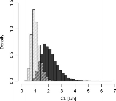
Distribution of individual CL values for males (dark grey) and females (light grey) after simulation of data for 10,000 males and 10,000 females

Simulation of Data Sets

Each data set consisted of data for 200 individuals, 60% of the individuals were randomly assigned to be males and 40% females. Two concentration measurements were simulated for each individual. Weights were simulated from two truncated log-normal distributions with sex-specific medians and variances (lnN(85.1, 0.0329) for males and lnN(73.0, 0.0442) for females) (Fig. 2) which had been estimated using a large data set with 1,022 males and 423 females [11]. Three missing data mechanisms were simulated: MCAR, MAR and MNAR. For each mechanism, 50% of the individuals were assigned to lack information about the covariate sex. For MCAR, all individuals had the same probability of missing sex; for MAR, the underlying mechanism gave a higher probability of missing sex with increasing weight (27% probability of missing sex for a person weighing 40 kg and 83% probability of missing sex for a person weighing 145 kg); and for MNAR, the underlying mechanism gave a three times higher probability of missing sex for males than females. The proportion of males in the data sets for whom sex was observed was then approximately 60% when data were MCAR, 56% when data were MAR and 37% when data were MNAR.

Fig. 2.

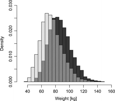
Distribution of individual weights for males (dark grey) and females (light grey) after simulation of data for 10,000 males and 10,000 females

Methods for Handling Missing Covariates

Six different methods for handling missing covariates were compared: complete case scenario (CC), single imputation of mode (SI_mode), single imputation based on weight (SI_WT), multiple imputation based on weight and individual response (i.e. Css_i) (MI), full maximum likelihood modelling using information on weight (MOD) and full maximum likelihood modelling where the proportion of males (and females) among the individuals lacking information about sex was estimated as an extra parameter in the model (EST). For comparison purposes, estimation with all data (ALL) was also conducted. Implementation of all methods except CC and SI_mode required estimation of additional models for logistic regression and MI also required additional simulations.

CC

All individuals lacking the covariate sex were excluded from the analysis, i.e. 50% of the data were discarded.

SI_mode

The mode of the covariate, i.e. the most frequently occurring category among the individuals for whom the covariate was observed, was imputed for all individuals lacking the covariate.

SI_WT

A model was created to describe the likelihood of being male given the observed weight (L(male|weight)). The model was estimated as a logistic regression among the individuals for whom both covariates were observed (NONMEM code in Appendix 1). The model was used together with the observed weights to predict the likelihood of being male for each individual. For all individuals for whom the information about sex was missing the covariate was imputed based on the individual likelihood prediction, i.e. a likelihood prediction greater than or equal to 0.5 was imputed as ‘male’, otherwise ‘female’ (NONMEM code in Appendix 1).

MI

The MI method presented by Wu and Wu [6] was implemented [12]. The PK model, without inclusion of any covariate (i.e. estimation of 1 fixed effect parameter instead of 2), was fitted to the data to get the CL_i for all individuals. CL_i contains information about the response variable (Css_i) [13,14] and can hence be used to create a model which describes the likelihood of being male given the observed weight and the response (L(male|weight,CL_i)). The likelihood model was estimated as a logistic regression among the individuals for whom the covariate was observed (NONMEM code in Appendix 1). For all individuals for whom the information about sex was missing, the covariate was imputed (simulated) based on the logistic regression model, the individuals’ observed weight and their individual estimate of CL (NONMEM code in Appendix 1). The imputation step followed by an estimation of the imputed data set was repeated six times for each data set. The six sets of population parameter estimates were combined to one set by calculating the average of the six point estimates of each fixed and random effect in the population model [12,15,16].

MOD

Based on the individuals for whom there were no missing covariate values, a model was created to describe the probability of being male given the observed weight (L(male|weight)). The probability model was used in a mixture model (for subjects for whom sex information was missing) together with the observed weights to provide the probability of being male for each individual (NONMEM code in Appendix 1). The mixture model functionality uses the individual responses, in combination with information on the probability of belonging to each of the subpopulations (in this case male or female) on the population level, to estimate the model parameters [8].

EST

Rather than fixing the expected relation between covariates to the estimates from the portion of the population without missing information, as in the MOD method, these relations were estimated. Thus, the fraction of individuals belonging to each subpopulation (i.e. the population likelihood of being male) was estimated as a fixed effect parameter in the mixture model. To ensure a hierarchical relation between EST and MOD the fixed effect parameter was added to the individual predicted probability of being male given the observed weight (the same likelihood model as was used in MOD) (NONMEM code in Appendix 1). The difference in objective function value (OFV) between the two models was then approximately χ ²-distributed and a decrease of at least 3.84 in OFV when adding the extra parameter was a significantly (p < 0.05) better fit of EST than MOD.

Comparison of Bias and Precision

Bias and precision of the estimated population parameters were evaluated by calculation and comparison of relative bias (RBias) and relative standard deviation (RSD), for each population parameter (i), under each method for handling the missing data (j; plus estimations using all data) and under each missing data mechanism (k).

The bias was defined as the deviation of the mean of the estimates from the true value and the RBias was calculated according to Eq. 3;

$$\mathrm{RBias}\left[P_{i,j,k}\right]=\frac{{\overline{P}}_{i,j,k}-P_i}{P_i}$$ 3

where $\overline{P}$ is the mean of the estimates of the parameter (fixed or random effect) and P is the corresponding true value, i.e. the value used in the simulation. All methods which resulted in parameter estimates with a RBias <5% for the fixed effect parameters, and <10% for the random effect parameters, were considered to be unbiased.

The RSD was used to describe the precision of the estimates relative the mean of the estimates of the parameter (Eqs. 4 and 5);

$$\mathrm{SD}\left[P_{i,j,k}\right]=\sqrt{\frac{1}{N-1}{\displaystyle {\sum }_{n=1}^N{\left({\widehat{P}}_{i,j,k}-{\overline{P}}_{i,j,k}\right)}^2}}$$ 4

$$\mathrm{RSE}\left[P_{i,j,k}\right]=\frac{\mathrm{SD}\left[P_{i,j,k}\right]}{{\overline{P}}_{i,j,k}}$$ 5

where SD is the standard deviation of the distribution of the estimates and N is the total number of estimates, i.e. the number of simulated data sets. All methods which resulted in parameter estimates with a RSD <10% for the fixed effect parameters, and <20% for the random effect parameters, were considered to give precise parameter estimates.

RESULTS

The bias and precision of the population parameter estimates, estimated using the different methods for handling the missing covariate, are presented in Tables I (RBias) and II (RSD). Bias and precision in estimates of the fixed effect of CL for males (CL_male) and females (CL_female) are also visualised in box plots, showing the bias as the deviation of the median estimate from the true value and the precision as the width of the box and the whiskers (Figs. 3, 4 and 5).

Table I.

Relative Bias (in Per Cent) in Population Parameter Estimates for the Different Methods When Data Were MCAR, MAR and MNAR

	MCAR				MAR				MNAR
	CLmale	CLfemale	BSV	ResErr	CLmale	CLfemale	BSV	ResErr	CLmale	CLfemale	BSV	ResErr
ALL	−0.32	−0.064	−1.7	0.82	−0.32	−0.064	−1.7	0.82	−0.32	−0.064	−1.7	0.82
EST	−0.37	−0.25	−1.6	0.82	−0.65	0.020	0.22	0.82	−0.41	−0.18	−1.4	0.82
MOD	−0.40	−0.10	−1.2	0.82	−0.88	−0.055	1.1	0.82	5.8	10	6.9	0.82
MI	−0.26	−0.054	−1.7	0.82	−0.69	0.14	0.75	0.82	5.2	6.2	−3.7	0.82
SIWT	−11	11	69	0.83	−11	10	69	0.83	−3.1	32	87	0.83
SImode	−16	0.24	78	0.82	−14	3.2	76	0.83	−0.90	42	110	0.83
CC	−0.14	0.022	−2.0	1.3	−0.27	0.18	−3.6	0.60	−0.90	−0.051	−2.9	1.4

The between-subject variability (BSV) and the residual error (ResErr) were estimated as variances

Table II.

Relative Standard Deviation (in Per Cent) in Population Parameter Estimates for the Different Methods When Data Were MCAR, MAR and MNAR

	MCAR				MAR				MNAR
	CLmale	CLfemale	BSV	ResErr	CLmale	CLfemale	BSV	ResErr	CLmale	CLfemale	BSV	ResErr
ALL	3.0	3.8	13	11	3.0	3.8	13	11	3.0	3.8	13	11
EST	3.4	4.6	15	11	3.7	4.5	15	11	3.6	4.2	16	11
MOD	3.4	4.5	15	11	3.5	4.4	15	11	3.5	4.7	17	11
MI	3.5	4.6	16	11	3.5	4.6	16	11	3.4	4.5	17	11
SIWT	3.7	6.2	12	11	3.8	6.3	13	11	4.7	4.7	12	11
SImode	3.9	6.1	11	11	6.3	10	12	11	5.4	3.6	11	11
CC	4.6	5.5	17	14	4.5	5.3	16	15	5.4	4.3	18	15

The between-subject variability (BSV) and the residual error (ResErr) were estimated as variances

Fig. 3.

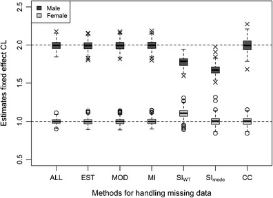
Box-plot showing bias and precision of the estimates of the typical value of CL for males (true value, 2) and females (true value, 1) after fitting 200 simulated data sets, in which the covariate sex was MCAR for 50% of the individuals, using six different methods to handle the missing data

Fig. 4.

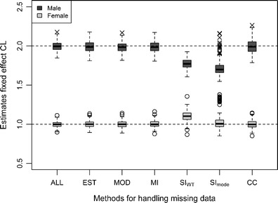
Box-plot showing bias and precision of the estimates of the typical value of CL for males (true value, 2) and females (true value, 1) after fitting 200 simulated data sets, in which the covariate sex was MAR for 50% of the individuals, using six different methods to handle the missing data

Fig. 5.

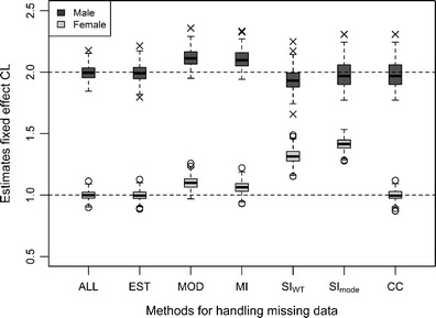
Box-plot showing bias and precision of the estimates of the typical value of CL for males (true value, 2) and females (true value, 1) after fitting 200 simulated data sets, in which the covariate sex was MNAR for 50% of the individuals, using six different methods to handle the missing data

CC

The method gave unbiased estimates for all population parameters, independent on underlying missing data mechanism (Table I). The estimates were less precise than the ones received using MI, MOD or EST but all RSDs were below the predefined limits (Table II) and should therefore be considered as precise. The estimates of the residual error were more biased and less precise when the CC method was used compared with when any of the other methods were used.

SI_mode

When data were MCAR or MAR, the SI_mode method resulted in considerably underestimated values of CL_male (RBias, −16% and −14%) while the estimates of CL_female remained unbiased but less precise than the estimates received with the more advanced methods (MI, MOD and EST) (Tables I and II; Figs. 3 and 4). More outliers were observed when data were MAR than when data were MCAR (Figs. 3 and 4), and this was also noticeable in the RSDs which were greater for CL_male and CL_female when data were MAR (Table II). When data were MNAR the estimates of CL_male were unbiased but less precise while the estimates of CL_female were highly overestimated (RBias, +42%) (Table I; Fig. 5). The estimates of the BSV were highly overestimated independent on missing data mechanism (RBias between +76% and +110%) (Table I). All population parameters were estimated with RSDs which were lower than the predefined limits, except CL_female which had a RSD of 10% when data were MAR.

SI_WT

When data were MCAR or MAR, the estimates of CL_male were underestimated (RBias, −11%) whereas the estimates of CL_female were overestimated (RBias, 11% and 10%) (Table I; Figs. 3 and 4). For the MNAR mechanism, the estimates of CL_male were unbiased according to the predefined limits (RBias, −3.1) (Table I) but the boxplot reveals a small underestimation (Fig. 5). The estimates of CL_female were highly overestimated (RBias, +32%) when data were MNAR (Table I; Fig. 5). The estimates of the BSV were highly overestimated independent on missing data mechanism (RBias between +69% and +87%) (Table I).

MI

This method gave unbiased and precise estimates of all population parameters when data were MCAR or MAR. When data were MNAR, the estimates of CL_male and CL_female were both overestimated (RBias, +5.2% for CL_male and +6.2% for CL_female) (Table I; Fig. 5). Both random effect parameters (BSV and residual error) were estimated without any bias and with high precision, independent on underlying missing data mechanism (Tables I and II).

MOD

The results received when using the MOD method were similar to those observed for the MI method. All population parameters were estimated without any bias and with high precision when data were MCAR or MAR. When data were MNAR, the estimates of CL_male and CL_female were both overestimated (RBias, +5.8% for CL_male and +10% for CL_female) (Table I; Fig. 5). The BSV and the residual error were estimated without bias and with high precision independent on the underlying missing data mechanism (Tables I and II).

EST

The EST method was the only method which gave unbiased and precise estimates of all population parameters independent on underlying missing data mechanism (Tables I and II; Figs. 3, 4 and 5). EST was significantly better than MOD in 8.5% of the simulated data sets when data were MCAR, in 13% of the data sets when data were MAR and in 100% of the data sets when data were MNAR. The extra parameter that was estimated in the EST method had a median estimate (median over the 200 simulated data sets) of 0 when data were MCAR or MAR whereas it had a median estimate of 2.0 when data were MNAR.

DISCUSSION

The relative differences in performance of the tested methods were very similar when data were MCAR and MAR, whereas most methods gave a greater bias in the estimates when data were MNAR. The more advanced methods (MI, MOD and EST) gave unbiased and precise estimates of all population parameters when data were MCAR or MAR. The only method giving unbiased and precise estimates even when data were MNAR was EST, followed by CC which gave unbiased but less precise estimates under all missing data mechanisms.

The lower precision in all population parameters when estimated with the CC method is because only 50% of the data were used in this analysis. There were no biases in the estimates of the population parameters as all data used in the analyses came from individuals for whom sex was observed, i.e. given the particular model used, the missing data were MCAR when analysed with the CC method, independent on missing data mechanism. However, when data are MAR or MNAR, CC is known to result in biased parameter estimates [2,5,17].

The incomplete data records contain a lot of information and if the analyst does not want to discard 50% of the data, there are many options and methods to choose in between. In single imputation, the missing values are filled in to achieve a complete data set without discarding any data. When the filled in data set is analysed in NONMEM, the imputed values are analysed as if they are the true values, without taking the uncertainty in the imputations into account. The shortcomings of this procedure is documented and discussed by Donner [18], Little and Rubin [2], Little [4] and Schafer and Graham [5]. In this study, two types of single imputation was included, SI_mode and SI_WT. The rationale for including these methods, even though they are observed to perform worse than full maximum likelihood methods and multiple imputations [4,5], was that these methods are common in nonlinear mixed effects modelling of clinical and pre-clinical data. The SI_mode method is equivalent to imputing the mean or median value of a continuous covariate and, as was shown in this study, this type of method underestimates the strength of the covariate–parameter relationship [2]. The underestimation of CL_male when data were MCAR or MAR (Table I; Figs. 3 and 4) was because in the majority of the simulated data sets, there were more males than females among the individuals for whom the sex was observed. All individuals with missing sex were then assumed to be males, but as some of them in fact were females, their lower CLs were downward biasing the estimates of CL_male. The same thing, but the other way around, happened when data were MNAR and CL_female was estimated with a positive bias (Table I; Fig. 5). The overestimation of the BSV (Table I) is a consequence of the large spread of individual estimates of CL when data from females were assumed to derive from males and vice versa. Despite the fact that the method underestimated the covariate–parameter relationship, the distributions of the estimates of CL_male and CL_female did not overlap each other which indicates that, in this case, the covariate would have been found significant even if SI_mode was the method used to handle the missing covariate.

A more advanced method to handle the missing covariate would be to derive a model for the covariate based on other, completely observed, covariates and then use that model for the imputation. This strategy was evaluated in this study by implementation of SI_WT and MI. SI_WT was a single imputation of sex based on the observed weight while MI was a multiple imputation of sex based on observed weight and the response variable (Css_i). The advantage of multiple imputations over single imputation is that the missing covariate values are imputed several times. Each of the filled in data sets are then analysed and the estimates are combined to receive one set of estimates, which means that the imputed values are not considered to be the true values and the uncertainty in the imputed values are taken into account [19]. When the missing data were handled with the SI_WT method, all estimates of the population parameters, except the estimates of the residual error, were biased. The CL_male parameter was always underestimated whereas the CL_female parameter and the BSV were overestimated (Table I; Figs. 3, 4 and 5). Despite the bias, the estimates were quite precise (RSE, 3.7–6.3%) which means that all the single imputed simulated data sets gave similar estimates. This indicates that the main problem with this method was that the correlation between weight and sex was weak and that a logistic regression model based on only weight gave a poor description of the individuals’ true sexes. The MI method used both the weight and information about the response as covariates in the logistic regression model and this resulted in unbiased estimates when data were MCAR or MAR (Table I; Figs. 3 and 4). The reason for this was not only because multiple imputations are better than single imputation but also because the response was more correlated with sex than weight. This can also be seen in Figs. 1 and 2 where the distributions of weights and the distributions of individual CL values (containing information about the response) for males and females are displayed. The weight distributions overlap each other to a larger extent than the distributions of the individual CL values do. The importance of including all variables which can be predictive of the missing covariate or the underlying missing data mechanism in the model for multiple imputations is discussed by Meng [20], Rubin [21] and Collins et al. [22]. These arguments should also be applicable to single imputation when the imputation is based on observed predictors in the data. Even if single imputation is a less proper procedure than multiple imputations when handling missing data, the differences between the methods would have been smaller if the same logistic regression model had been used for simulating the single imputations.

The MOD method gave estimates similar to those received using the MI method. Both methods gave unbiased and precise estimates of all population parameters when data were MCAR or MAR, wheras the estimates of CL_male and CL_female were overestimated when data were MNAR (Tables I and II; Figs. 3, 4 and 5). The overestimation of both these parameters was due to the difference in fraction of males in the part of the data set where sex was observed for all individuals (37% males) and the part where information about sex was missing (83% males). As the fraction of males was low in the part of the data set where sex was observed the logistic regression models (both the one used in MI and the one used in MOD) were assigning all individuals a relatively low likelihood of being male independent on body weight and/or individual estimates of CL. The MI method was therefore imputing fewer males than females in total, and males with a lower body weight and/or a lower individual estimate of CL were more likely to be imputed as females than males with a higher body weight and/or a higher individual estimate of CL. Therefore, there was a positive bias in both the estimates of CL_female and the estimates of CL_male. When modelling the missing data using a mixture model (as in MOD) and the probability of male versus female is different for the population with missing covariate information compared with the rest of the population, there will be a bias in the underlying probability model for which parameters are fixed. This bias will influence the parameters that are estimated. Thus, the mechanisms giving rise to bias in MOD and MI when covariates are MNAR are essentially the same.

Methods using multiple imputations or full maximum likelihood modelling yield similar results when handling missing data in linear fixed effect models, when the methods are implemented in comparable ways [4,5,22]. The same relative performance is expected for nonlinear mixed effect models. The efficiency of multiple imputation methods depends on the number of imputed data sets and between two and ten imputations are enough to get the point estimates near their minimum sampling variance on repeated sampling from the population of interest [15] but more imputations might be needed if the fraction of missing information is large [16]. Other important inferential quantities such as null hypothesis significance tests, p values and confidence interval half-widths can suffer from substantial imprecision when just a few number of imputations are used [23]. In this study, the focus was on the point estimates of the population parameters and as the fraction of missing information was assumed to be quite low, six imputations were considered appropriate. The MI and MOD methods both use the individual weights and responses when fitting the data sets, MI in the logistic regression model used in the imputation of missing sexes and MOD when maximising the likelihood of the individuals’ sexes using information on their weight, and hence they produce similar results.

The hierarchical relation established between EST and MOD made it possible to compare the methods’ OFVs. A significant drop in OFV when EST was used instead of MOD indicated that the individual likelihood predictions (based on the individuals’ weight) used in the mixture model had poor predictability. This could be due to data being MNAR but could also be the result of a logistic regression model with poor predictability. When data were MCAR or MAR, then EST was in most cases not significantly better than MOD, but when data were MNAR, then EST was significantly better than MOD for 100% of the simulated data sets.

Rubin shows that when a proper method is used (e.g. multiple imputations or maximum likelihood modelling) to analyse data where some information is missing and the missing data are MCAR or MAR, the missing data mechanism can be ignored [1]. When data are MNAR, the underlying missing data mechanism is no longer ignorable and a model describing the mechanism has to be included in the analysis to enable unbiased estimates [1,24]. However, the underlying missing data mechanism is usually unknown and the model will therefore rely on the assumptions made by the analyst. In this study, the missing data mechanism was not included in the analysis using any of the methods which means that the data were assumed to be MCAR or MAR. The extra fixed effect parameter which was estimated when using the EST method compensated for the MNAR mechanism, and EST was the only method tested which gave unbiased and precise estimates independent on missing data mechanism. When analysing data where a large extent of the individuals are lacking information about one covariate or more, estimation of this extra parameter should be used to evaluate the predictability of the developed (logistic) regression model before any conclusions can be drawn from the estimated parameters. The inclusion of the extra parameter should be based on goodness of fit such as the OFV.

Multiple imputations and full maximum likelihood modelling of continuous missing covariates can be done in a similar way as multiple imputations and full maximum likelihood modelling of categorical missing covariates. A regression model with observed covariates (and information about the response if it is for multiple imputations) is created for the missing covariate and a random effect is added to the regression model and estimated to take the uncertainty in the model into account. For multiple imputations, the imputations are then created by using the regression model and drawing (i.e. simulating) random values from the estimated uncertainty distribution [12]. For full maximum likelihood modelling, the variance of the uncertainty distribution is fixed to the estimated value and the values of the missing covariates are estimated from the fixed distribution and the individuals’ observed data.

The covariate effect simulated in this study was incorporated as an effect of the binary covariate sex on drug CL. The choice of covariate name was arbitrary and the simulated missing data mechanisms and/or the proportions of males/females in the simulated data sets should not be given any physiological meaning. A real-life situation when categorical covariate data are MAR is for example during pooled analyses when some covariates have not been measured/reported during one of the studies, and a real-life example of when categorical covariate data are MNAR is when individuals with a high alcohol consumption are less willing to grade their alcohol intake than individuals with a lower alcohol consumption.

The population PK model used in this study was very simple and a more complex model with more population parameters to estimate would result in less precise estimates than what was seen in this study. This would be true even if no data are missing and a more complex model would therefore make the observed differences between the methods less obvious. Sex had a large influence on the individual CL values, and at the same time, a large proportion of the individuals were lacking information about the covariate. These settings were chosen to emphasise the differences between the tested methods, and even though the observed differences might be smaller if the model is more complex, the covariate is less influential and/or the fraction of individuals lacking information about the covariate is smaller, the relative differences between the methods will still remain. The covariate under study was categorical, but the same relative performances of the CC, MI, MOD and EST methods are expected for continuous covariates since the models in the continuous case builds on virtually the same statistical principles. As there is no round off to the nearest category in the continuous case, the continuous counterparts of the SI_mode and SI_WT methods are expected to perform relatively better but still not as well as MI, MOD and EST.

This analysis evidence that there is a large difference in efficiency of the tested methods and that care has to be taken when deciding which method to be used for the analysis of missing covariates in nonlinear mixed effects modelling.

CONCLUSIONS

The study shows that MI, MOD and EST are good approaches to receive precise and unbiased estimates in the presence of missing data when the underlying missing data mechanism is MCAR or MAR. If the data are MNAR, the only method resulting in low bias and high-parameter precision is EST.

APPENDIX 1

Implementation of methods for handling missing covariate data in NONMEM:

Population Model

The population model used for simulations and estimations:where MALE is the sex covariate (1 if male and 0 if female), CL is the drug clearance and Y is the response variable, i.e. the log-transformed steady-state concentrations.

Regression Models

The likelihood/logistic regression model, run before SI_WT, MOD and EST, evaluated by analysis on data records where no data were missing: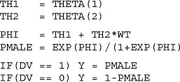where WT is body weight and PMALE is the probability of being male given a specific weight.

The likelihood/logistic regression model, run before MI, evaluated by analysis on data records where no data were missing: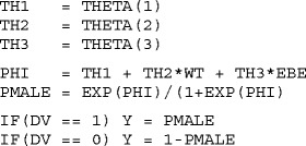where WT is body weight, EBE is the individual empirical Bayes estimates of CL, and PMALE is the probability of being male given a specific weight and a specific individual estimate of CL.

SI_WT

The imputation model:where IMALE stands for ‘imputed male’ which was the sex covariate used in the model if the observed sex covariate MALE was missing.

MI

The imputation model: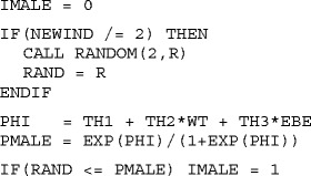where RAND is a random value from the uniform distribution [0, 1] and IMALE stands for imputed male which was the sex covariate used in the model if the observed sex covariate MALE was missing.

MOD

The mixture model/estimation model: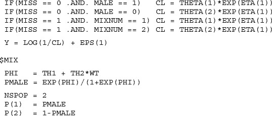where MISS is a missing data indicator (0 if the data record is complete (i.e. the covariate is not missing) and 1 if the data record is incomplete), MALE is the (partly) observed sex covariate, MIXNUM is the index of the subpopulation for which variables are to be computed (1 for male and 2 for female) and $MIX describes the mixture model with the prior information from the logistic regression model.

Note that the parameters of the logistic regression model can be estimated directly in the mixture model/estimation model. The reason why this was not done in this study was because the methods were compared using the SSE option of the mimp (multiple imputation) functionality in PsN where MOD was tested as an alternative model (i.e. fitted to a data set where the parameters of the logistic regression model were already available).

EST

The mixture model/estimation model: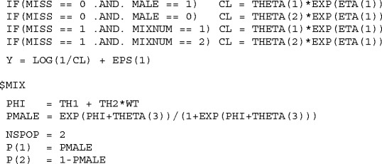where MISS is a missing data indicator (0 if the data record is complete (i.e. the covariate is not missing) and 1 if the data record is incomplete), MALE is the (partly) observed sex covariate, MIXNUM is the index of the subpopulation for which variables are to be computed (1 for male and 2 for female) and $MIX describes the mixture model with the prior information from the logistic regression model.

Note that the parameters of the logistic regression model can be estimated directly in the mixture model/estimation model. The reason why this was not done in this study was because the methods were compared using the SSE option of the multiple imputation functionality in PsN where EST was tested as an alternative model (i.e. fitted to a data set where the parameters of the logistic regression model were already available).

References

- 1.Rubin DB. Inference and missing data. Biometrika. 1976;63(3):581–592. doi: 10.1093/biomet/63.3.581. [DOI] [Google Scholar]
- 2.Little RJA, Rubin DB. Statistical analysis with missing data. 2. New Jersey: Wiley; 1987. [Google Scholar]
- 3.Orchard T, Woodbury MA, editors. A missing information principle: theory and applications. In: Proc Sixth Berkeley Symp Math Stat Probab. 1972.
- 4.Little RJA. Regression with missing X’s: a review. J Am Stat Assoc. 1992;87:1227–1237. [Google Scholar]
- 5.Schafer JL, Graham JW. Missing data: our view of the state of the art. Psychol Methods. 2002;7(2):147. doi: 10.1037/1082-989X.7.2.147. [DOI] [PubMed] [Google Scholar]
- 6.Wu H, Wu L. A multiple imputation method for missing covariates in non-linear mixed-effects models with application to HIV dynamics. Stat Med. 2001;20:1755–1769. doi: 10.1002/sim.816. [DOI] [PubMed] [Google Scholar]
- 7.Bonate PL. Pharmacokinetic-pharmacodynamic Modeling and Simulation. US: Springer; 2011. [Google Scholar]
- 8.Beal S, Sheiner LB, Boeckmann A, Bauer RJ. NONMEM User’s Guides. (1989–2009) Ellicott City: ICON Development Solutions; 2009. [Google Scholar]
- 9.Lindbom L, Ribbing J, Jonsson EN. Perl-speaks-NONMEM (PsN)—a Perl module for NONMEM related programming. Comput Methods Programs Biomed. 2004;75(2):85–94. doi: 10.1016/j.cmpb.2003.11.003. [DOI] [PubMed] [Google Scholar]
- 10.Lindbom L, Pihlgren P, Jonsson N. PsN-Toolkit—a collection of computer intensive statistical methods for non-linear mixed effect modeling using NONMEM. Comput Methods Programs Biomed. 2005;79(3):241–257. doi: 10.1016/j.cmpb.2005.04.005. [DOI] [PubMed] [Google Scholar]
- 11.Tunblad K, Lindbom L, McFadyen L, Jonsson EN, Marshall S, Karlsson MO. The use of clinical irrelevance criteria in covariate model building with application to dofetilide pharmacokinetic data. J Pharmacokinet Pharmacodyn. 2008;35(5):503–526. doi: 10.1007/s10928-008-9099-z. [DOI] [PubMed] [Google Scholar]
- 12.Johansson ÅM, Karlsson MO. Multiple imputation of missing covariates in NONMEM and evaluation of the method’s sensitivity to η-shrinkage. AAPS J. 2013 doi: 10.1208/s12248-013-9508-0. [DOI] [PMC free article] [PubMed] [Google Scholar]
- 13.Maitre P, Bührer M, Thomson D, Stanski D. A three-step approach combining Bayesian regression and NONMEM population analysis: application to midazolam. J Pharmacokinet Pharmacodyn. 1991;19(4):377–384. doi: 10.1007/BF01061662. [DOI] [PubMed] [Google Scholar]
- 14.Mandema JW, Verotta D, Sheiner LB. Building population pharmacokinetic-pharmacodynamic models. I. Models for covariate effects. J Pharmacokinet Pharmacodyn. 1992;20(5):511–528. doi: 10.1007/BF01061469. [DOI] [PubMed] [Google Scholar]
- 15.Rubin DB. Multiple Imputation for Nonresponse in Surveys. New York: Wiley; 1987. [Google Scholar]
- 16.Schafer JL. Analysis of incomplete multivariate data. London: Chapman & Hall; 1997. [Google Scholar]
- 17.Harrell FE. Regression modeling strategies: with applications to linear models, logistic regression, and survival analysis. Berlin: Springer; 2001. [Google Scholar]
- 18.Donner A. The relative effectiveness of procedures commonly used in multiple regression analysis for dealing with missing values. Am Stat. 1982;36:378–381. [Google Scholar]
- 19.Rubin DB, editor. Multiple imputations in sample surveys—a phenomenological Bayesian approach to nonresponse. In: Proceedings of the survey research methods section. American Statistical Association; 1978.
- 20.Meng XL. Multiple-imputation inferences with uncongenial sources of input. Stat Sci. 1994;9:538–558. [Google Scholar]
- 21.Rubin DB. Multiple imputation after 18+ years. J Am Stat Assoc. 1996;91:473–489. doi: 10.1080/01621459.1996.10476908. [DOI] [Google Scholar]
- 22.Collins LM, Schafer JL, Kam CM. A comparison of inclusive and restrictive strategies in modern missing data procedures. Psychol Methods. 2001;6(4):330. doi: 10.1037/1082-989X.6.4.330. [DOI] [PubMed] [Google Scholar]
- 23.Bodner TE. What improves with increased missing data imputations? Struct Equ Model. 2008;15(4):651–675. doi: 10.1080/10705510802339072. [DOI] [Google Scholar]
- 24.Gastonguay MR, French JL, Heitjan DF, Rogers JA, Ahn JE, Ravva P. Missing data in model-based pharmacometric applications. J Clin Pharmacol. 2010;50(9 suppl):63S–74S. doi: 10.1177/0091270010378409. [DOI] [PubMed] [Google Scholar]