High-accuracy prediction of transmembrane inter-helix contacts and application to GPCR 3D structure modeling

Abstract

Motivation: Residue–residue contacts across the transmembrane helices dictate the three-dimensional topology of alpha-helical membrane proteins. However, contact determination through experiments is difficult because most transmembrane proteins are hard to crystallize.

Results: We present a novel method (MemBrain) to derive transmembrane inter-helix contacts from amino acid sequences by combining correlated mutations and multiple machine learning classifiers. Tested on 60 non-redundant polytopic proteins using a strict leave-one-out cross-validation protocol, MemBrain achieves an average accuracy of 62%, which is 12.5% higher than the current best method from the literature. When applied to 13 recently solved G protein-coupled receptors, the MemBrain contact predictions helped increase the TM-score of the I-TASSER models by 37% in the transmembrane region. The number of foldable cases (TM-score >0.5) increased by 100%, where all G protein-coupled receptor templates and homologous templates with sequence identity >30% were excluded. These results demonstrate significant progress in contact prediction and a potential for contact-driven structure modeling of transmembrane proteins.

Availability: www.csbio.sjtu.edu.cn/bioinf/MemBrain/

Contact: hbshen@sjtu.edu.cn or zhng@umich.edu

Supplementary information: Supplementary data are available at Bioinformatics online.

1 INTRODUCTION

Membrane proteins constitute ∼30% of the proteins in both prokaryotic and eukaryotic genomes (Adamian and Liang, 2006), and they participate in various crucial cellular processes, from basic small-molecule transport to complicated signaling pathways (Elofsson and von Heijne, 2007). It has been shown that >50% of current drug targets are membrane proteins (Hopkins and Groom, 2002), where the top four gene families of Food and Drug Administration-approved drugs are all membrane proteins; i.e. G protein-coupled receptor (GPCR), nuclear receptors, ligand-gated ion channels and voltage-gated ion channels (Overington et al., 2006). Membrane-embedded alpha-helical polytopic proteins constitute the majority of ion channels, transporters and receptors in living organisms. This class of proteins, which accounts for ∼40% of all membrane proteins, is infamously difficult for high-resolution structural studies. Due to the intrinsic structural plasticity associated with many of these proteins, the chance of obtaining crystals suitable for X-ray or electron diffraction studies is small (Yarov-Yarovoy et al., 2006). Although helical membrane proteins have many experimental difficulties, their structural conformation has been demonstrated to be predictable in a number of ways, e.g. transmembrane helix (TMH) domain topology (Krogh et al., 2001; Shen and Chou, 2008).

Structure prediction of the TMH bundle for alpha-helical membrane proteins can be fulfilled by first predicting TMHs and then applying helix-packing constraints (White, 2003). The first step of the TMH prediction has a long history, and the current methods can achieve an accuracy of ∼90% (Nugent and Jones, 2009; Shen and Chou, 2008). In the second step, it has been widely acknowledged that residue–residue contact maps contain crucial constraints for ab initio assembly of protein structures. In the past 5 years, several methods have been proposed to predict inter-TMH residue contacts and TMH–TMH interactions from the primary sequence. These approaches generally can be classified into two categories: (i) correlated mutation analysis (CMA)-based approaches [e.g. HelixCorr (Fuchs et al., 2007)], and (ii) machine learning (ML)-based methods [e.g. TMHcon (Fuchs et al., 2009), TMhit (Lo et al., 2009), MEMPACK (Nugent and Jones, 2010) and TMhhcp (Wang et al., 2011)]. CMA-based approaches identify co-evolving residue pairs that tend to be in contact from multiple sequence alignments (MSAs). ML-based methods predict inter-TMH residue contacts by training statistical models using various sequence-derived features. The predicted contacts are used to predict TMH–TMH interactions. Despite the progress, there is much space for improvement.

First, in the case of CMA-based approaches, the performance depends highly on the number of aligned sequences in MSAs. For example, the recent CMA-based residue contact prediction algorithm PSICOV (Jones et al., 2012) performs poorly on the CASP hard targets, which tend to have few homologous sequences (Di Lena et al., 2012). This indicates that contact prediction based on CMA alone is insufficient. Second, from ML point of view, inter-TMH residue contact prediction is an imbalanced learning problem, where the number of samples in different classes (contact versus non-contact) differs significantly. Existing ML-based methods use random under-sampling (He and Garcia, 2009) to select the negative samples. Except for random forest in TMhhcp (Wang et al., 2011), which used 100 decision trees, all the existing predictors were trained with a single model using a 1:1 or 1:4 ratio of contact and non-contact samples. There is no single best ML algorithm because each has a different mathematical hypothesis. Therefore, an ensemble classifier constructed by applying multiple algorithms on multiple training sets can combine the diversities among different predictors and yield better results (Shen and Chou, 2006). Third, in all the existing ML-based models, feature vectors of two residues are serially concatenated together. Although this serial combination is widely used, the doubled feature vector dimensions may decrease performance due to over-fitting effects of high-dimensional data. The parallel strategy is another feature fusion approach (Yang et al., 2003), which represents the two vectors as real and imaginary parts in a complex space. The benefit is that the dimension of the obtained complex vector is the same as the vector of each residue, which we show improves performance.

In this study, we present a novel method called MemBrain to predict inter-TMH residue contacts by merging an ML-based engine with the CMA-based approach. Here, we use the PSICOV (Jones et al., 2012) algorithm to calculate correlated mutation scores (CMs). The ML-based engine in the proposed protocol is implemented with an ensemble classifier. It is the fusion of five OET-KNN (Zouhal and Denoeux, 1998) classifiers and five SVM classifiers, where each independent classifier is trained with a different training set obtained from five independent under-samplings. By doing so, we can get the diversities from different algorithms and, at the same time, reduce the information loss via multiple samplings.

2 MATERIALS AND METHODS

2.1 Data sets

For fair comparison, we used the same two benchmark data sets from previous studies. The training data set was taken from TMHcon (Fuchs et al., 2009) consisting of 62 alpha-helical transmembrane (TMH) proteins. Here, we only used 60 of these proteins and discarded 1l7vA and 1vf5B because of either non-standard atomic coordinate records or too few positive contacts, as defined in the next section. All the 60 proteins have at least three TMHs with the pairwise sequence identity <40% among the training data set. TMH locations and their topologies were extracted from the databases of TOPDB (Tusnady et al., 2008), PDBTM (Tusnady et al., 2005) and OPM (Lomize et al., 2006). For extra validation, an independent data set was taken from TMhhcp (Wang et al., 2011), which contains 21 TMH proteins with the pairwise sequence identity <40% in itself and to the training data set.

2.2 Contact definition and evaluation criteria

We adopted the contact definition from TMHcon (Fuchs et al., 2009), MEMPACK (Nugent and Jones, 2010) and TMhhcp (Wang et al., 2011) for the convenience of direct comparisons with these methods. Briefly, two residues from different TMHs are considered to be in contact if the minimal distance of their side chain or backbone heavy atoms is <5.5 Å.

In this work, we evaluated our method using a leave-one-out jackknife cross-validation, which is the same as previous studies. It takes one protein sequence out for testing, while keeping the remaining protein sequences for training. This procedure will be terminated when all the proteins have been tested individually. The overall prediction performance was evaluated by averaging the performances on individual proteins. We also assessed our method using a 4-fold cross-validation, where the four equal-size subsets have roughly the same number distribution of TMHs. Additionally, we used an independent data set for further validation. In this case, the final model was trained based on the whole training data set.

For inter-TMH residue contact prediction, the top L/5-predicted contacts were selected for assessing the prediction performance and then used to determine TMH–TMH interactions, which is the same as previous reports (Fuchs et al., 2009). Here, L is the length of the concatenate TMHs. Concretely, three measures are used to evaluate the performance, i.e. Accuracy, Coverage and Accuracy (δ = 4). Accuracy is defined as the fraction of correctly predicted contacts with respect to all the predicted contacts. Coverage is defined as the percentage of correctly predicted contacts from the total observed contacts. Accuracy (δ = 4) is derived from δ-analysis (Ortiz et al., 1999), which calculates the fraction of predicted contacts lying within one helix turn (four residues each side) around the observed contacts.

For TMH–TMH interaction prediction, interacting helix pairs were derived from the top L/5-predicted contacts. As defined in previous studies, a helix pair is considered to be interacting if it contains at least one contact. Applying this definition to the training/independent data set, we obtained 681/334 interacting helix pairs and 757/347 non-interacting helix pairs, respectively, where the ratios between interacting and non-interacting samples are similar to previous reports (Nugent and Jones, 2010). Based on the observed interactions, the performance of predicting TMH–TMH interactions can then be assessed. Four measures are used to evaluate the performance, i.e. Accuracy, Sensitivity, Specificity and MCC. Here, Accuracy is defined as the fraction of correctly predicted interactions with respect to all the predicted interactions.

2.3 Feature extraction

We extracted four types of sequence-based features, including position-specific scoring matrix (PSSM), residue position, relative position within TMH and sequence separation between two residues, for model training. TMH locations and their topologies were extracted from annotated databases. Details for each type of input features are described in the following text:

2.3.1 Position-specific scoring matrix

The PSSM of each protein was generated by using PSI-BLAST (Altschul et al., 1997) program to search against the UniRef90 database with three iterations and an E-value threshold of 0.001. PSSM can be represented by an L by 20 matrix, where L is the protein length. To consider neighboring residues, a sliding window centered on a target residue, with four residues on each side of that residue, was used to extract a 180-dimensional feature vector. The original score in each position was normalized by the following logistic function of Equation (1) (Fuchs et al., 2009):

(1)

where x is the original score.

2.3.2 Residue position

A 10-dimensional binary vector is used to encode the residue position along the TMH to reflect the contact site. The first seven vector elements correspond to seven equally split parts along the TMH. These elements were set to 0, other than the element at index calculated by Equation (2) defined as follows:

(2)

where N denotes the length of the TMH containing the target residue, and p denotes the position of the target residue between 1 and N on the TMH. Here, the function f returns the floor value. The vector element at index was set to 1 if the target residue is in the index-th part of the helix. The last three vector elements indicate which side of the TMH the residue lies on. We divided each TMH into three parts to encode whether the residue lies closest to the cytoplasmic side ([1 0 0]), helix core ([0 1 0]) or extracellular side ([0 0 1]). One-quarter of the TMH consists of the cytoplasmic side, another quarter the extracellular side and the remaining the helix core.

2.3.3 Residue relative position

Residue relative position was calculated by Equation (3) defined as follows:

(3)

where N and p are as previously described, and i stands for the i-th TMH along the protein sequence from N- to C-terminal. Residues with similar position and relative position may have similar membrane bilayer depth.

2.3.4 Sequence separation

Sequence separation was encoded by a nine-dimensional binary vector corresponding to the number of residues between two residues. The bins consist of less than 25, 50, 75, 100, 125, 150, 175, 200 and more than 200 residues. If the separation satisfied the threshold corresponding to the vector element j, then all vector elements no more than j were set to 1.

2.4 Feature fusion

2.4.1 Serial combination

The most straightforward way to combine the two feature vectors from candidate residue pair is to serially concatenate one after the other, as implemented in all the previous studies (Fuchs et al., 2009; Lo et al., 2009; Nugent and Jones, 2010; Wang et al., 2011). Suppose that the feature vectors x and y represent residues i and j, respectively, the serially combined feature vector z is a real vector defined as follows:

(4)

2.4.2 Parallel combination

The symmetry of feature vectors of the two residues motivates us to investigate a parallel combination approach (Yang et al., 2003). Given the two feature vectors x and y described earlier, the parallelly combined feature vector z is a complex vector instead of the real vector in Equation (4), which is defined as follows:

(5)

where i represents an imaginary unit.

2.4.3 Feature reduction

Many different kinds of feature reduction algorithms are available, and among them the principle component analysis (PCA) algorithm is widely used (Fukunaga, 1990). However, for the parallel combination in complex space [Equation (5)], PCA cannot be directly used. An extension of PCA called GPCA (generalized principle component analysis) has been proposed (Yang et al., 2003) for dealing with the complex vector feature reduction problem. Suppose that the complex feature vector z lies in a unitary space, let Q be the number of pattern classes, P(ω_i) be the prior probability of pattern class i, be the mean feature vector of pattern class i and be the mean vector of all the feature vectors. The between-class scatter matrix, within-class scatter matrix and total-scatter matrix are, respectively, defined as follows:

(6)

(7)

(8)

From Equations (6–8), it is obvious that S_b, S_w and S_t are all semi-positive definite Hermite matrices, so together with the proved theorem that each eigenvalue of Hermite matrix is a real number (Ding and Cai, 1995), we then can have the following corollary: the eigenvalues of S_b, S_w and S_t in unitary space are all non-negative real numbers. Based on the aforementioned corollary, the GPCA thus can be described as follows: Let v₁, v₂, … , v_n be the orthogonal eigenvectors of S_t, and λ₁, λ₂, … , λ_n be the associated eigenvalues, which satisfy λ₁≥λ₂≥ … ≥λ_n. By choosing the first m-maximal eigenvectors as projection axes, a given feature vector z can be projected to an m-dimensional vector g by Equation (9) as follows:

(9)

where Φ = (v₁, v₂, … , v_m). The dimensionality-reduced vector g, rather than the original combined feature vector z, is then used for classification. Note that the dimensionality-reduced vector g also lies in a unitary space. When the complex feature space degenerates to a real space, the GPCA is in fact the classic PCA.

2.5 Prediction model

The developed MemBrain predictor is composed of two engines: CMA-based and ML-based prediction modules. The flowchart of MemBrain is shown in Figure 1. The merit of CMA-based engine is that it has a clear biophysical interpretation, but its performance is highly dependent on the number of homologous sequences. The ML-based engine is not easily interpretable, but it handles the small-sample problem better. These two engines complement each other in inter-TMH residue contact prediction to drive MemBrain as an accurate prediction model.

Fig. 1.

Flow chart of residue contact prediction protocol in MemBrain

2.5.1 CMA-based prediction engine

Approaches that use CMs to detect co-evolving residue pairs work commonly through calculating the Pearson correlation coefficient (Gobel et al., 1994; Pollock and Taylor, 1997) or mutual information (Burger and van Nimwegen, 2010; Dunn et al., 2008) between columns in MSAs. PSICOV (Jones et al., 2012), a recent approach that is based on mutual information, improved significantly the accuracy of contact prediction by using a sparse inverse covariance estimation technique (Meinshausen and Buhlmann, 2006) to deal with indirect coupling effects.

We used PSICOV to calculate CMs, where the residue pairs that lie on the same TMH were removed. The initial MSAs were collected by using PSI-BLAST to search against the UniRef90 database with three iterations and an E-value threshold of 0.001. In the final alignments, all columns not belonging to any TMH regions were deleted and duplicate sequences were also discarded. The output raw scores were scaled to the range [0, 1] using the standardized function:

(10)

where x is the raw score and min and max are minimal and maximal scores for a given protein.

2.5.2 ML-based prediction engine

Applying the contact definition described earlier, we obtained 11 526 contact residue pairs (positive samples) and 532 531 non-contact residue pairs (negative samples). The ratio between the total contact pairs and all the non-contact pairs is ∼1:46, resulting in the problem of imbalanced learning. In principle, we can randomly sample a subset from the negative class and incorporate it with all positive samples to form a relative balanced training set. However, the information loss induced by random under-sampling will weaken the prediction performance. In light of this problem, we applied ensemble learning to reduce the impact of under-sampling.

We randomly sampled five subsets from the negative class independently and incorporated each subset with all positive samples to generate five different training sets. These five training sets were used to train five separate OET-KNN and SVM classifiers. The ratio between the positives and the sampled negatives is important because it will serve as a base for the statistical algorithm to learn the distributions of different classes. According to our experiments, the ratio 1:4 between positive and negative samples for each protein gives better performance and hence is used in MemBrain. OET-KNN and SVM classifiers were trained with parallel fused feature sets and serial combined feature sets, respectively, because our experimental results show that this is a better choice, and meanwhile, strong diversities can be generated among the component classifiers, which are critical for ensemble learning performance (Zhou and Yu, 2005).

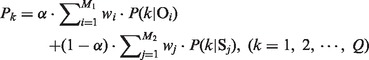
We have trained multiple classifiers consisting of five OET-KNN classifiers and five SVM classifiers, which were fused together with a linear combination scheme based on posteriori probabilities. To give a general definition, suppose that there exist M₁ OET-KNN classifiers, M₂ SVM classifiers and Q pattern classes, we then define the linear combination scheme as follows:

(11)

where P(k|O_i) and P(k|S_j) denote the probability of class k by the i-th OET-KNN classifier and the j-th SVM classifier, respectively; P_k denotes the fused probability; w_i and w_j denote the weights of the i-th OET-KNN classifier and the j-th SVM classifier, respectively, which are set to the average value for all members of the same classifier type, i.e. w_i = 1/M₁ and w_j = 1/M₂. The weight α is selected by searching the value from 0 to 1 with a step of 0.01 via a jackknife cross-validation. Obviously here, M₁ = M₂ = 5 and Q = 2. Note that the raw scores generated by each classifier for a given protein were scaled to the range [0, 1] with Equation (10) before combination. This ensemble ML predictor is denoted as OSC (OET-KNN and SVM Classifier).

2.5.3 Final prediction model

The combination of CMA-based engine PSICOV and ML-based ensemble engine OSC forms the final prediction model, which is implemented in MemBrain. The outputs of OSC and PSICOV are merged by using a linear combination defined as follows:

(12)

where P_OSC and P_PSICOV are the predicted contact probabilities generated by OSC and PSICOV, respectively, and P denotes the final contact propensity. The weight β is selected using the same search strategy as the weight α.

3 RESULTS

3.1 Benchmark test of CMA-based approach

We applied the CMA-based algorithm PSICOV (Jones et al., 2012) for inter-TMH residue contact prediction. It was performed on the concatenated sequence, which consists of the TMH regions. Residue pairs that lie on the same TMH were removed from the predictions. All the possible residue pairs were ranked according to the generated CMs. The top ranked L/5 residue pairs were selected as the predicted contacts, where L is the total number of residues in the TMHs.

PSICOV calculates CMs from MSAs by PSI-BLAST search through the UniRef90 database. The quality of MSAs is critically important for the final prediction accuracy. Supplementary Figure S1 illustrates the average performance of PSICOV on 60 TMH proteins in the training data set. As can be seen, the prediction performance is highly dependent on sufficient homology. When the number of homologous sequences increases from 250 to 5000, the prediction accuracy improves as well from 21.6 to 42.1%. Although the performance can be improved by including more homologous sequences, there is a limit. We have tried to increase this parameter to greater than 5000, but found that the prediction performance did not change much. For a balance, we set the parameter of -b to 5000 for PSI-BLAST in the following experiments. With this parameter, the prediction accuracy is 42.1% on the training data set.

To examine the effects of MSAs’ size on accuracy, we divided the training data set into five subsets based on the number of sequences in MSAs. The performance of residue contact prediction on these five subsets is shown in Supplementary Table S1. As expected, better performance was achieved for proteins with a larger set of MSAs (52.8% in Group 5 with more than 5000 aligned sequences), whereas poorer performance for those with smaller MSAs (12.8% in Group 1 with less than 250 aligned sequences). In the case of difficult targets that have few homologous sequences, the prediction of residue contacts is still a challenge to PSICOV due to the incorrect co-evolution values that are calculated from small MSAs. For instance, the average accuracy on the five proteins in Group 1 with no more than 250 homologous sequences found is only 12.8%, with a coverage rate as low as 3.4%. These results demonstrate the weakness of the CMA-based approach.

3.2 Benchmark test of ML-based engine

We have trained five OET-KNN classifiers (denoted as OET1, OET2, OET3, OET4 and OET5) (see Supplementary Fig. S2) and five SVM classifiers (denoted as SVM1, SVM2, SVM3, SVM4 and SVM5), where each of them was trained with different training sets. As shown in Supplementary Table S2, the prediction accuracy of exact contacts by individual OET-KNN classifiers varies from 45.5 to 47.8% and that with a residue variation within one helix turn (δ = 4) ranges from 78.0 to 78.5%. For individual SVM classifiers, the prediction accuracy varies from 46.9 to 49.0% and that with δ = 4 ranges from 83.1 to 85.2%. These results indicate that the prediction performance is unstable with respect to classification algorithm and the sampling. When we combined individual OET-KNN classifiers with equal weights, denoted as OETs, the prediction accuracy increased to 48.2%. Similarly, we combined individual SVM classifiers, denoted as SVMs, the prediction accuracy improved to 50.7%. As shown in Supplementary Figure S3, the areas under the curve of the combined classifiers OETs and SVMs are 0.805 and 0.841, which are superior to those of the individual OET-KNN and SVM classifiers, respectively.

Both of the improvements by OETs and SVMs demonstrate that fusing multiple classifiers is an effective way to reduce the information loss in the under-sampling process. Thus, we constructed an ensemble predictor called OSC by combining OETs and SVMs to make full use of diversities from multiple training subsets and classification algorithms according to Equation (11). Supplementary Figure S4A illustrates the results.

The combination of OETs and SVMs indeed performs better on small weights as expected because SVMs performs better than OETs. At first as the weight α increases, the prediction performance improves, and then it degrades to the performance of OETs. When α increases to the value 0.24, the highest prediction accuracy of 52.8% is obtained, which is then adopted in the ensemble classifier. As shown in Supplementary Table S2, OSC performs better than both OETs and SVMs on all the three measures. The prediction accuracy of OSC is 4.6% higher than OETs and 2.1% higher than SVMs. The area under the curve of OSC is 0.846, which is higher than 0.805 of OETs and 0.841 of SVMs (Supplementary Fig. S3). The good performance of OSC is due to the complementation of individual classifiers.

3.3 Merging CMA-based approach with ML-based engine

As the predicted CMs indicate the potential of residue pairs to form contacts, this information can be used not only as features but also as decisions. In Supplementary Table S3, we show that decision-level fusion (regarding CMs as independent prediction) discussed in this article outperforms feature-level fusion (regarding CMs as an additional feature fed into the ML model) applied in existing methods in both cases of OET-KNN and SVM. For instance, in the case of OET-KNN, feature-level fusion does not help to improve the performance, whereas decision level fusion improves the accuracy from 47.8 to 57.0%. Thus, we constructed a consensus predictor to further improve the prediction performance by merging the outputs of ensemble classifier OSC and PSICOV (Jones et al., 2012), which is implemented as MemBrain according to Equation (12). As shown in Supplementary Figure S4B, the highest prediction accuracy was obtained when the weight β is 0.56. The prediction accuracy of the consensus predictor is 62.0%, as listed in Supplementary Table S2.

The combination of OSC and PSICOV significantly improves the prediction performance in terms of all the three measures. The complementation contributes 9.2% prediction accuracy and 5.1% accuracy (δ = 4) to OSC. The consensus predictor achieves 19.9% higher prediction accuracy than PSICOV alone. We also analyzed statistical significance of the differences of the three criteria between MemBrain and OSC/PSICOV using a paired t-test. If the resulting P-value is below a level (e.g. 0.05), the performance difference between two methods is considered to be statistically significant. The resulting p-values in terms of accuracy, coverage and accuracy (δ = 4) are 1.2e-4/4.2e-7, 3.4e-3/2.6e-6 and 6.5e-3/1.7e-7, respectively. These results indicate that MemBrain is statistically better than the other two independent engines.

Supplementary Table S1 also shows the performance of MemBrain on five groups of proteins according to MSAs’ size. Comparing with PSICOV, we find that accuracies in all the five groups are improved (see Fig. 2). The largest improvement occurs in Group 2, where the accuracy is increased from 28.0 (PSICOV) to 73.5% (MemBrain). For the very difficult targets in Group 1, the accuracy is increased from 12.8 to 23.6%. These results show that the combination of OSC and PSICOV is helpful for fusing the merits of both ML-based and CMA-based methods to enhance the prediction accuracy. Supplementary Figure S5 elucidates how OSC and PSICOV complement each other by taking two TMH proteins 1bccC and 2nr9A as instances.

Fig. 2.

Performance improvement on five groups by combining OSC to PSICOV

3.4 Performance comparison of residue contact prediction with existing methods

In this section, we compared our predictor MemBrain with existing methods on both training and independent data sets, including three inter-TMH residue contact predictors [TMHcon (Fuchs et al., 2009), MEMPACK (Nugent and Jones, 2010) and TMhhcp (Wang et al., 2011)] and two globular protein residue contact predictors [SVMcon (Cheng and Baldi, 2007) and SVMSEQ (Wu and Zhang, 2008)]. On the training data set, the compared predictors for TMH proteins are evaluated on the same data set with jackknife cross-validation. On the independent data set, experimental results of TMHcon and MEMPACK were taken from TMhhcp. PSICOV (Jones et al., 2012) is also included for comparison. TMhhcp reported two types of results based on all the features and the selected features (denoted as TMhhcp1 and TMhhcp2), we list both of them for comparison. For globular protein contact predictors, we only ranked the residue pairs that lie on different TMHs.

As shown in Table 1, MemBrain performs substantially better than other methods, with a prediction accuracy of 62.0%/64.1% on the training/independent data set. Note that MEMPACK selected the predicted contacts based on scores generated by the SVM predictor rather than the top L/5 predictions, and the coverage is the fraction of the total correctly predicted contacts from all the observed contacts and hence is larger than the methods based on the top L/5 predictions. Taking the best existing method TMhhcp for comparison, MemBrain achieves 12.5%/16.0% and 16.2%/15.5% higher prediction accuracy than TMhhcp1 and TMhhcp2, respectively, on the training/independent data set, and the corresponding prediction accuracy (δ = 4) is 6.5%/5.2% and 6.6%/7.8% higher. It is noteworthy that globular protein contact predictors SVMcon and SVEMSEQ perform poorly when applied to TMH proteins. We also conducted the paired t-test to compare the statistical significance between MemBrain and SVMcon/SVMSEQ on the training data set. The resulting p-values in terms of accuracy, coverage and accuracy (δ = 4) are 1.9e-21/2.5e-19, 1.1e-17/4.9e-15 and 1.9e-12/1.8e-11, respectively. These results suggest that predictors designed for globular proteins are not suitable for predicting inter-TMH residue contacts. The reason can be the very different cellular environments of residues in and out of the membrane, and hence the features are also different. In addition, we also assessed our method using a 4-fold cross-validation and obtained comparable results with that of jackknife cross-validation. Supplementary Table S4 shows the performance on more non-redundant data sets.

Table 1.

Performance comparison of residue contact prediction

Method	Accuracy (%)	Coverage (%)	Accuracy (δ = 4) (%)
Comparison on the training data set
TMHcon	25.9	3.5	78.5
TMhhcp1	49.5	8.2	83.9
TMhhcp2	45.8	7.4	83.8
SVMcon	8.4	1.5	55.1
SVMSEQ	13.0	2.8	60.9
PSICOV	42.1	6.7	74.7
MemBraina	61.4	10.1	89.1
MemBrainb	62.0	10.2	90.4
Comparison on the independent data set
TMHcon	23.6	3.0	83.4
MEMPACK	36.2	10.4	63.0
TMhhcp1	48.1	6.1	84.4
TMhhcp2	48.6	6.1	81.8
SVMcon	10.4	1.6	68.0
SVMSEQ	17.7	2.4	66.0
PSICOV	50.9	6.6	81.1
MemBrain	64.1	8.3	89.6

Note: ^aResults obtained from 4-fold cross-validation.

^bResults obtained from jackknife cross-validation.

Interestingly, PSICOV performs better on the independent data set than the training data set, as shown in Table 1, where the prediction accuracy is improved from 42.1 to 50.9%. We found that 26 of 60 proteins from the training data set contained less than 1000 aligned sequences in MSAs, whereas for the independent data set, the ratio is 3 of 21. In addition, 10 proteins in the training data set contained less than 500 aligned sequences, whereas all the proteins in the independent data set contained more than 500 aligned sequences. The results demonstrate that the performance of PSICOV is highly dependent on sufficient homology.

3.5 Performance comparison of TMH–TMH interaction prediction with existing methods

One important use of the predicted contacts is to identify interacting TMHs. Using the observed interactions described previously, the performance of TMH–TMH interaction prediction can be assessed. The performance comparison with existing methods is shown in Supplementary Table S5. MemBrain achieves 90.1%/87.9% prediction accuracy and an MCC of 0.555/0.526 on the training/independent data set, which performs better than the existing methods. As TMH interaction prediction is derived from the predicted contacts, globular protein contact predictors perform poorly on inter-TMH residue contact prediction and thus are not as good as the TMH protein contact predictors for TMH–TMH interaction prediction. Also, as can be seen from Supplementary Figure S5, the predicted contacts obtained by PSICOV (Jones et al., 2012) are widespread. In other words, it predicted more interacting TMH pairs with higher sensitivity. Meanwhile, it predicted more spurious interacting TMH pairs as well with lower accuracy, which resulted in a relative lower MCC compared with MemBrain.

3.6 Benchmark test on MemBrain-guided GPCR structure modeling

To have a direct examination of the impact of the MemBrain contact predictions on three-dimensional (3D) GPCR modeling, we collected all 13 GPCR proteins with known structure in the PDB library (PDBID: 1u19A, 2rh1A, 2y00A, 2z73A, 3emlA, 3oduA, 3pblA, 3rzeA, 3vw7A, 4dajA, 4djhA, 4ea3A, 4grvA, see Table 2). We then generate GPCR models by I-TASSER (Roy et al., 2010; Xu et al., 2011) with MemBrain contacts and also models without using MemBrain contacts.

Table 2.

Protein structure modeling of 13 GPCRs by I-TASSER with or without using MemBrain contact predictions with RMSD and TM-score calculated in the transmembrane regions^a

PDBID	Lb	LTMc	Acc (L/5)d	Acc (L)e	RMSD/ TMf	RMSD/ TMg
1u19A	348	169	0.52	0.36	9.9/0.547	7.1/0.667
2rh1A	282	180	0.58	0.35	20.7/0.208	11.6/0.498
2y00A	286	180	0.61	0.35	6.7/0.466	5.0/0.604
2z73A	350	181	0.69	0.46	18.0/0.213	8.7/0.687
3emlA	286	186	0.35	0.25	19.1/0.196	18.6/0.315
3oduA	282	182	0.72	0.36	6.7/0.615	4.4/0.771
3pblA	272	174	0.59	0.36	15.1/0.287	15.5/0.398
3rzeA	267	176	0.57	0.31	14.4/0.243	5.1/0.616
3vw7A	284	182	0.56	0.36	9.4/0.552	8.2/0.634
4dajA	264	177	0.54	0.30	4.1/0.729	3.7/0.806
4djhA	286	177	0.57	0.37	5.9/0.686	5.2/0.768
4ea3A	278	177	0.51	0.29	5.7/0.669	3.9/0.803
4grvA	298	182	0.61	0.36	5.9/0.634	4.4/0.719
Average	291	178	0.57	0.35	10.9/0.465	7.8/0.637

Note: ^aAll GPCR templates and homologous templates with sequence identity >30% were excluded.

^bNumber of residues of the whole chain.

^cNumber of residues in the transmembrane regions.

^dAccuracy of the top L/5 contact predictions by MemBrain.

^eAccuracy of the top L contact predictions used by I-TASSER.

^fRMSD (Å) and TM-score of the first model by I-TASSER without using MemBrain predictions.

^gRMSD (Å) and TM-score of the first model by I-TASSER using MemBrain predictions.

Although MemBrain contact predictions are only on the C_α atoms, we found that the best GPCR models can be generated when the same contact restraints are extended for all C_α, C_β and side-chain center of mass in the I-TASSER simulations. Table 2 summarized the results of I-TASSER with and without using MemBrain contacts, where all GPCR templates and the homologous templates with a sequence identity >30% or detectable by PSI-BLAST are excluded. First, although no GPCR templates were used, the inherent I-TASSER fragment assembly simulation was able to assemble structures with an approximately correct TMH arrangement (TM-score >0.5) in 7 of 13 cases; in 5 cases, the models have a TM-score >0.6. The average TM-score and RMSD to the X-ray structure are 0.465 and 10.9 Å, respectively, in the TMH regions.

The average accuracy of the MemBrain contact predictions is 0.57 for the top L/5 predictions, whereas I-TASSER uses the top L contacts, which have an average accuracy of 0.35. As shown in Table 2, the incorporation of MemBrain contacts has significantly improved the quality of the GPCR models. For example, the number of cases with a TM-score >0.6 increases from 5 to 10 and the average TM-score increases by 37%. This TM-score improvement on GPCRs by MemBrain contacts is dramatically higher than that observed on the globular proteins by SVMSEQ (Wu and Zhang, 2008) contacts for the I-TASSER models, which have a TM-score increase by 4.6% (Wu et al., 2011). The major reason for the difference is the higher accuracy of the long-range contacts by MemBrain, which have been specifically trained for TMHs. If we apply SVMSEQ on the 13 GPCRs, the average accuracy of contacts is only 0.16 for top L/5 or 0.09 for top L predictions (not to mention that many of the SVMSEQ predictions are short-range contacts, which are less useful for protein 3D constructions).

As expected, there is an obvious correlation between the TM-score improvement and the accuracy of the MemBrain contacts. For the targets with the most significant improvement (e.g. 2z73A and 3rzeA), the accuracy of MemBrain for the top L contacts is 46 and 31%, respectively. For targets of relatively lower accuracy (3emlA with a contact accuracy 25%), the TM-score of the I-TASSER models is slightly improved but still in the unfoldable region (TM-score = 0.315). There are some targets, e.g. 4djhA, where the MemBrain contact accuracy is high (0.57 for L/5 and 0.37 for L), but the TM-score improvement (12%) is lower than average because a high proportion of MemBrain contacts (78%) are already included in the I-TASSER models. Nevertheless, the remaining 22% of the novel contacts from MemBrain serve to refine the models.

In Figure 3, we present the superposition of MemBrain-guided I-TASSER models and X-ray structures for all 13 GPCRs. Most of the I-TASSER models indeed show a similar topology of TMH packing to the targets. However, there are a few targets (e.g. 2z73A, 3pblA and 4djhA) where the I-TASSER models have the TMH structure bended away from the axis at the middle of the helices. This is due to the fact that the I-TASSER simulations were fully automated and no TMH requirements were implemented. Thus, the bended helices from non-homologous templates resulted in the helix bending. If TMH predictions from MEMSTAT (Jones et al., 1994) were used, the TMH bending could be eliminated but the overall TM-score was not obviously improved (data not shown).

Fig. 3.

Superposition of the first model (blue) and the X-ray structure (red) in the transmembrane regions for 13 known GPCRs. Models are generated by I-TASSER with contact restraints from MemBrain. All GPCR templates and the homologous templates with a sequence identity >30% detectable by PSI-BLAST have been excluded during I-TASSER simulations

Although the MemBrain contacts are only in the TMH regions, the overall I-TASSER models along the entire chain are also improved. As shown in Supplementary Table S6 and Supplementary Figure S6, the average TM-score of the whole-chain models is increased by 35% and RMSD reduced by 2.6 Å. The number of targets with a correct fold (TM-score >0.5) increases from 5 to 10, when the MemBrain contact predictions are used. It is worth mentioning that all GPCR templates and homologous templates with sequence identity >30% were both excluded in aforementioned I-TASSER simulations. If we only excluded the homologous templates with sequence identity >30% in I-TASSER simulations, in which case some GPCR templates can be kept, then the final average RMSD is as low as 1.8 Å with a TM-score 0.902, as demonstrated in Supplementary Table S7.

3.7 Case studies

The usefulness of MemBrain contact predictions has been demonstrated in the case of GPCR 3D structure modeling. To further demonstrate the effectiveness of MemBrain contact predictions for other TMH proteins besides GPCRs, we performed structure prediction for two newly solved membrane protein structures, i.e. heterodimeric ABC transporter (3qf4A) (Hohl et al., 2012) and channelrhodopsin (ChR) chimera between ChR1 and ChR2 (3ug9A) (Kato et al., 2012). The pairwise sequence identities of the two proteins to the training data set are <30%. Using MemBrain, 64.5 and 80.7% of the predicted top L/5 contacts are native contacts for the two proteins, respectively. Their corresponding accuracies derived from δ-analysis (δ = 4) are both 100%. These results are shown in Supplementary Figure S7.

Similar to the GPCR benchmark, homologous templates were removed. We first tried removing templates that have sequence identity >30%. In both proteins when contact predictions were not used, the RMSD in the TMH region was 4.3 and 3.0 Å for 3qf4A and 3ug9A, respectively. The results are given in Table 3. For both proteins, the accuracy without predicted contacts is already high. Although MemBrain predictions are good relative to current contact prediction methods, the probability of improving these structures further with predicted contacts is small, and the structures may even be made slightly worst. This was indeed the case for both proteins (Table 3), where no improvement occurred. Nevertheless, contact prediction can improve structures of mediocre quality, so we also tried removing templates that have sequence identity >15% to generate these structures for improvement.

Table 3.

The top I-TASSER model (largest cluster) for 3qf4A and 3ug9A with or without using MemBrain contact predictions

PDBID	Cutoff	RMSD/ TMa	RMSD/ TMb	RMSD/ TMc	RMSD/ TMd
3qf4A	30e	4.3/0.607	4.2/0.610	6.1/0.715	6.0/0.716
	15e	4.2/0.605	4.2/0.606	25.3/0.437	23.0/0.449
	A15f	6.7/0.523	4.6/0.600	26.0/0.422	25.4/0.417
	50g	16.7/0.264	16.5/0.261	22.2/0.288	22.0/0.286
3ug9A	30e	3.0/0.795	3.2/0.765	15.0/0.649	14.9/0.642
	15e	5.6/0.524	4.2/0.599	12.5/0.450	11.9/0.500
	A15f	10.9/0.369	5.3/0.600	19.9/0.323	16.0/0.500
	50g	15.0/0.219	6.9/0.564	17.4/0.231	16.3/0.472

Note: The RMSD and TM-score to native for different degrees of template structure removal are given.

^aRMSD (Å) and TM-score in the TMH region without using MemBrain predictions.

^bRMSD (Å) and TM-score in the TMH region using MemBrain predictions.

^cRMSD (Å) and TM-score of the whole chain without using MemBrain predictions.

^dRMSD (Å) and TM-score of the whole chain using MemBrain predictions.

^eTemplates whose sequence has >X% sequence identity to the protein were removed.

^fAverage results of the top 10 models, where templates whose sequence has >15% sequence identity to the protein were removed.

^gTemplates whose structure has TM-score >0.5 to the native structure were removed.

For 3qf4A, in the 15% sequence identity case, the resulting model without MemBrain contacts remained similar at 4.2 Å in the TMH region, but the RMSD of the entire chain increased significantly by >19.0 Å relative to the 30% case. With MemBrain contacts, the RMSD in the TMH region also remained similar at 4.2 Å, and the whole-chain RMSD increased by 17.0 Å. Although the predicted contacts did not have much effect on the first model, the contacts did reduce the number of poorly predicted structures among the top 10 models. Without the predicted contacts, the two worst models were 9.9 and 20.4 Å; whereas with the contacts, the worst model was 5.5 Å, which makes the significant improvement in the top 10 models in terms of both the average RMSD and TM-score (Table 3). It is worth pointing out that 3qf4A is an especially challenging case because it is a dimer, and the helices that span the membrane also protrude significantly outside the membrane to form an intracellular domain. In addition to inter-chain contacts, inter-helix contacts were not predicted for the residues outside the membrane, which limited the accuracy of helix placement and reduced the impact of MemBrain contact predictions.

For 3ug9A, in the 15% sequence identity case, the result was 5.6 and 4.2 Å in the TMH region, respectively, for the case without and with MemBrain-predicted contacts. As to the top 10 models, the MemBrain-predicted contacts are found also helpful by improving the average RMSD from 10.9 to 5.3 Å, with TM-score improved from 0.369 to 0.6.

To challenge MemBrain further, templates with TM-score >0.5 to the X-ray structure were removed to increase the dependence on the predicted contacts rather than on the templates for protein folding. In this case, the improvement was significant for 3ug9A, where the change was from 15.0 to 6.9 Å in the TMH region. We tried the same >0.5 cutoff for 3qf4A, but the result was >16 Å in the TMH region for both cases because of the lack of inter-helical contact information in the intracellular domain.

4 DISCUSSION

Our results demonstrate that the weakness of CMA (sufficient homology) can be compensated for by combining it with ML methods, and the weakness of statistical ML (local condensed predictions) can also be complemented by combining with CMA-based approaches. It would be interesting to investigate whether the idea of combining ML-based methods with CMA-based approaches in MemBrain can also be used to enhance the contact prediction accuracy in globular proteins. To demonstrate this, we used PSI-BLAST to search against UniRef90 database for the 22 targets containing free modeling or free modeling/template-based modeling domains in CASP9. Supplementary Figure S8 shows the distributions of the number of homologous sequences on the CASP9 targets.

The results in Supplementary Figure S8 demonstrate: (i) Although some targets have very few or no homologous structures in the PDB, which causes difficulties for homology structure modeling, they have a large number of homologous sequences available. For example, four of these targets have more than 1000 homologous sequences in the UniRef90 database. This means we can get reliable predicted contacts for these four proteins (∼61% average accuracy for top L/5 predictions on the training data set). (ii) In the other 18 targets, 9 of them contain less than 250 homologous sequences. According to our results, the accuracy of PSICOV in this group was very low (12.8% in this work), and the combination of ML-based method with PSICOV is expected to improve the accuracy (23.6% in this work). Furthermore, there are six proteins in the homology size region of (250 500). When directly applying PSICOV on this group, the results are also not satisfactory (28.0% in this work). However, the MemBrain prediction significantly improves the results in this group (73.5% in this work).

To further illustrate the potential merit of the combination of ML-based methods with CMA-based approaches on globular proteins, we replaced the ML-part of the MemBrain predictor with SVMSEQ. The predictions of SVMSEQ for the 22 targets were extracted from http://www.predictioncenter.org/download_area/CASP9/predictions/, which were merged with PSICOV outputs using a linear combination strategy. Supplementary Table S8 lists the detailed performance of top L/5 predictions for each range contact on the 22 targets. As can be seen, the performance improved as expected. From the results, it is very interesting to see the following: SVMSEQ performs better than PSICOV on the short-range contacts (33.6% versus 12.8%), and worse than PSICOV on the long-rang contacts (17.1% versus 20.3%). This is consistent with our previous observation that the ML-based approach gives more local condensed predictions. The results also show that SVMSEQ and PSICOV predictions are largely complementary on long-range contacts, which makes the combination of them more accurate. These results suggest that a proper consensus of CMA-based approaches with ML-based methods is also promising for enhancing the ab initio contact predictions in globular proteins.

Besides inter-TMH residue contacts in TMHs (denoted as Type 1), there exist two other contact types in TMH proteins: contacts where one residue is in the membrane region and the other residue in the water-soluble loop region (denoted as Type 2), and contacts where both residues are in the water soluble region (denoted as Type 3). These two types of contacts are also important for 3D structure prediction, especially for the loop region. By observing the native contacts from known structures in the training and the independent data set at the whole-chain level, we found that 48.0 and 45.9% are Type 3 contacts, and 14.1 and 14.8% are Type 2 contacts. Hence, predicting these two types of contacts will be important future work. In this case, the predictors developed for predicting residue contacts in globular proteins are expected to contribute.

Funding: The National Natural Science Foundation of China (61222306, 91130033, 61175024), Shanghai Science and Technology Commission (11JC1404800), a Foundation for the Author of National Excellent Doctoral Dissertation of PR China (201048), the National Science Foundation Career Award (DBI 0746198) and the National Institute of General Medical Sciences (GM083107, GM084222).

Conflict of Interest: none declared.

REFERENCES

- Adamian L, Liang J. Prediction of transmembrane helix orientation in polytopic membrane proteins. BMC Struct. Biol. 2006;6:13. doi: 10.1186/1472-6807-6-13. [DOI] [PMC free article] [PubMed] [Google Scholar]
- Altschul SF, et al. Gapped BLAST and PSI-BLAST: a new generation of protein database search programs. Nucleic Acids Res. 1997;25:3389–3402. doi: 10.1093/nar/25.17.3389. [DOI] [PMC free article] [PubMed] [Google Scholar]
- Burger L, van Nimwegen E. Disentangling direct from indirect co-evolution of residues in protein alignments. PLoS Comput. Biol. 2010;6:e1000633. doi: 10.1371/journal.pcbi.1000633. [DOI] [PMC free article] [PubMed] [Google Scholar]
- Cheng J, Baldi P. Improved residue contact prediction using support vector machines and a large feature set. BMC Bioinformatics. 2007;8:113. doi: 10.1186/1471-2105-8-113. [DOI] [PMC free article] [PubMed] [Google Scholar]
- Di Lena P, et al. Deep architectures for protein contact map prediction. Bioinformatics. 2012;28:2449–2457. doi: 10.1093/bioinformatics/bts475. [DOI] [PMC free article] [PubMed] [Google Scholar]
- Ding XR, Cai MK. Matrix Theory in Engineering. Tianjin: Tianjin University Press; 1995. [Google Scholar]
- Dunn SD, et al. Mutual information without the influence of phylogeny or entropy dramatically improves residue contact prediction. Bioinformatics. 2008;24:333–340. doi: 10.1093/bioinformatics/btm604. [DOI] [PubMed] [Google Scholar]
- Elofsson A, von Heijne G. Membrane protein structure: prediction versus reality. Annu. Rev. Biochem. 2007;76:125–140. doi: 10.1146/annurev.biochem.76.052705.163539. [DOI] [PubMed] [Google Scholar]
- Fuchs A, et al. Co-evolving residues in membrane proteins. Bioinformatics. 2007;23:3312–3319. doi: 10.1093/bioinformatics/btm515. [DOI] [PubMed] [Google Scholar]
- Fuchs A, et al. Prediction of helix–helix contacts and interacting helices in polytopic membrane proteins using neural networks. Proteins. 2009;74:857–871. doi: 10.1002/prot.22194. [DOI] [PubMed] [Google Scholar]
- Fukunaga K. Introduction to Statistical Pattern Recognition. San Diego: Academic Press; 1990. [Google Scholar]
- Gobel U, et al. Correlated mutations and residue contacts in proteins. Proteins. 1994;18:309–317. doi: 10.1002/prot.340180402. [DOI] [PubMed] [Google Scholar]
- He HB, Garcia EA. Learning from imbalanced data. IEEE Trans. Knowl. Data Eng. 2009;21:1263–1284. [Google Scholar]
- Hohl M, et al. Crystal structure of a heterodimeric ABC transporter in its inward-facing conformation. Nat. Struct. Biol. 2012;19:395–402. doi: 10.1038/nsmb.2267. [DOI] [PubMed] [Google Scholar]
- Hopkins AL, Groom CR. The druggable genome. Nat. Rev. Drug Discov. 2002;1:727–730. doi: 10.1038/nrd892. [DOI] [PubMed] [Google Scholar]
- Jones DT, et al. A model recognition approach to the prediction of all-helical membrane protein structure and topology. Biochemistry. 1994;33:3038–3049. doi: 10.1021/bi00176a037. [DOI] [PubMed] [Google Scholar]
- Jones DT, et al. PSICOV: precise structural contact prediction using sparse inverse covariance estimation on large multiple sequence alignments. Bioinformatics. 2012;28:184–190. doi: 10.1093/bioinformatics/btr638. [DOI] [PubMed] [Google Scholar]
- Kato HE, et al. Crystal structure of the channelrhodopsin light-gated cation channel. Nature. 2012;482:369–374. doi: 10.1038/nature10870. [DOI] [PMC free article] [PubMed] [Google Scholar]
- Krogh A, et al. Predicting transmembrane protein topology with a hidden Markov model: application to complete genomes. J. Mol. Biol. 2001;305:567–580. doi: 10.1006/jmbi.2000.4315. [DOI] [PubMed] [Google Scholar]
- Lo A, et al. Predicting helix–helix interactions from residue contacts in membrane proteins. Bioinformatics. 2009;25:996–1003. doi: 10.1093/bioinformatics/btp114. [DOI] [PMC free article] [PubMed] [Google Scholar]
- Lomize MA, et al. OPM: orientations of proteins in membranes database. Bioinformatics. 2006;22:623–625. doi: 10.1093/bioinformatics/btk023. [DOI] [PubMed] [Google Scholar]
- Meinshausen N, Buhlmann P. High-dimensional graphs and variable selection with the lasso. Ann. Stat. 2006;34:1436–1462. [Google Scholar]
- Nugent T, Jones DT. Transmembrane protein topology prediction using support vector machines. BMC Bioinformatics. 2009;10:159. doi: 10.1186/1471-2105-10-159. [DOI] [PMC free article] [PubMed] [Google Scholar]
- Nugent T, Jones DT. Predicting transmembrane helix packing arrangements using residue contacts and a force-directed algorithm. PLoS Comput. Biol. 2010;6:e1000714. doi: 10.1371/journal.pcbi.1000714. [DOI] [PMC free article] [PubMed] [Google Scholar]
- Ortiz AR, et al. Ab initio folding of proteins using restraints derived from evolutionary information. Proteins. 1999;37:177–185. doi: 10.1002/(sici)1097-0134(1999)37:3+<177::aid-prot22>3.3.co;2-5. [DOI] [PubMed] [Google Scholar]
- Overington JP, et al. How many drug targets are there? Nat. Rev. Drug Discov. 2006;5:993–996. doi: 10.1038/nrd2199. [DOI] [PubMed] [Google Scholar]
- Pollock DD, Taylor WR. Effectiveness of correlation analysis in identifying protein residues undergoing correlated evolution. Protein Eng. 1997;10:647–657. doi: 10.1093/protein/10.6.647. [DOI] [PubMed] [Google Scholar]
- Roy A, et al. I-TASSER: a unified platform for automated protein structure and function prediction. Nat. Protoc. 2010;5:725–738. doi: 10.1038/nprot.2010.5. [DOI] [PMC free article] [PubMed] [Google Scholar]
- Shen HB, Chou JJ. MemBrain: improving the accuracy of predicting transmembrane helices. PLoS One. 2008;3:e2399. doi: 10.1371/journal.pone.0002399. [DOI] [PMC free article] [PubMed] [Google Scholar]
- Shen HB, Chou KC. Ensemble classifier for protein fold pattern recognition. Bioinformatics. 2006;22:1717–1722. doi: 10.1093/bioinformatics/btl170. [DOI] [PubMed] [Google Scholar]
- Tusnady GE, et al. PDB_TM: selection and membrane localization of transmembrane proteins in the protein data bank. Nucleic Acids Res. 2005;33:D275–D278. doi: 10.1093/nar/gki002. [DOI] [PMC free article] [PubMed] [Google Scholar]
- Tusnady GE, et al. TOPDB: topology data bank of transmembrane proteins. Nucleic Acids Res. 2008;36:D234–D239. doi: 10.1093/nar/gkm751. [DOI] [PMC free article] [PubMed] [Google Scholar]
- Wang XF, et al. Predicting residue-residue contacts and helix-helix interactions in transmembrane proteins using an integrative feature-based random forest approach. PLoS One. 2011;6:e26767. doi: 10.1371/journal.pone.0026767. [DOI] [PMC free article] [PubMed] [Google Scholar]
- White SH. Translocons, thermodynamics, and the folding of membrane proteins. FEBS Lett. 2003;555:116–121. doi: 10.1016/s0014-5793(03)01153-0. [DOI] [PubMed] [Google Scholar]
- Wu S, et al. Improving protein structure prediction using multiple sequence-based contact predictions. Structure. 2011;19:1182–1191. doi: 10.1016/j.str.2011.05.004. [DOI] [PMC free article] [PubMed] [Google Scholar]
- Wu S, Zhang Y. A comprehensive assessment of sequence-based and template-based methods for protein contact prediction. Bioinformatics. 2008;24:924–931. doi: 10.1093/bioinformatics/btn069. [DOI] [PMC free article] [PubMed] [Google Scholar]
- Xu D, et al. Automated protein structure modeling in CASP9 by I-TASSER pipeline combined with QUARK-based ab initio folding and FG-MD-based structure refinement. Proteins. 2011;79:147–160. doi: 10.1002/prot.23111. [DOI] [PMC free article] [PubMed] [Google Scholar]
- Yang J, et al. Feature fusion: parallel strategy vs. serial strategy. Pattern Recognit. 2003;36:1369–1381. [Google Scholar]
- Yarov-Yarovoy V, et al. Multipass membrane protein structure prediction using Rosetta. Proteins. 2006;62:1010–1025. doi: 10.1002/prot.20817. [DOI] [PMC free article] [PubMed] [Google Scholar]
- Zhou ZH, Yu Y. Ensembling local learners through multimodal perturbation. IEEE Trans. Syst. Man Cybern. 2005;35:725–735. doi: 10.1109/tsmcb.2005.845396. [DOI] [PubMed] [Google Scholar]
- Zouhal LM, Denoeux T. An evidence-theoretic k-NN rule with parameter optimization. IEEE Trans. Syst. Man Cybern. 1998;28:263–271. [Google Scholar]
Associated Data
This section collects any data citations, data availability statements, or supplementary materials included in this article.