Powerful Regression-Based Quantitative-Trait Linkage Analysis of General Pedigrees

Abstract

We present a new method of quantitative-trait linkage analysis that combines the simplicity and robustness of regression-based methods and the generality and greater power of variance-components models. The new method is based on a regression of estimated identity-by-descent (IBD) sharing between relative pairs on the squared sums and squared differences of trait values of the relative pairs. The method is applicable to pedigrees of arbitrary structure and to pedigrees selected on the basis of trait value, provided that population parameters of the trait distribution can be correctly specified. Ambiguous IBD sharing (due to incomplete marker information) can be accommodated in the method by appropriate specification of the variance-covariance matrix of IBD sharing between relative pairs. We have implemented this regression-based method and have performed simulation studies to assess, under a range of conditions, estimation accuracy, type I error rate, and power. For normally distributed traits and in large samples, the method is found to give the correct type I error rate and an unbiased estimate of the proportion of trait variance accounted for by the additive effects of the locus—although, in cases where asymptotic theory is doubtful, significance levels should be checked by simulations. In large sibships, the new method is slightly more powerful than variance-components models. The proposed method provides a practical and powerful tool for the linkage analysis of quantitative traits.

Introduction

The Haseman-Elston (H-E) method of quantitative-trait linkage analysis for sib-pair data is based on regression of squared trait difference on the estimated proportion of alleles shared identical-by-descent (IBD) at a marker locus (Haseman and Elston 1972). This method has the advantages of simplicity and robustness (Allison et al. 2000) but is less powerful than variance-components (VC) models (Fulker and Cherny 1996). Several groups have recently proposed modifications to the original H-E method, to improve its power (Wright 1997; Drigalenko 1998; Elston et al. 2000; Xu et al. 2000; Forrest 2001; Sham and Purcell 2001; Visscher and Hopper 2001). In addition to the squared difference, these methods also use the squared sum of mean-centered trait values. Sham and Purcell (2001) showed that weighting the squared sum and squared difference by the inverse of their variances leads to a test that has similar power to VC. The method retains the advantages of the original H-E regression method in being computationally less demanding than VC and, more importantly, is more suited to the analysis of selected samples, which are collected in the vast majority of linkage studies.

Given that linkage studies typically are not simple sib-pair designs, it would be desirable to develop a general method of quantitative trait locus (QTL) linkage analysis that can accommodate larger sibships and complex pedigrees, while retaining the advantages of the regression-based methods. In a recent review on QTL linkage analysis, Feingold (2001) concludes that a key question that remains to be answered is “…whether there is a procedure (existing or to be discovered) that can retain the robustness and computational convenience of Haseman-Elston regression while approaching the greater power of variance components methods.” Here, we outline a novel procedure with these desirable properties. This method involves regression of multipoint IBD sharing on trait squared sums and squared differences, among all pairs of relatives. The method takes into account that IBD information may be incomplete, as is always the case with real data. We also report the results of simulation studies that demonstrate the properties of the method in terms of power, as compared with that of VC, and its robustness to model misspecification, non-normality, and phenotypic selection.

Method

Nonparametric linkage analysis is based on the relation of IBD sharing at a putative locus to some function of trait values. The most fundamental assumption of the proposed method is that most of the linkage information in a pedigree is summarized by pairwise relationships: pairwise identity-by-descent (IBD) sharing at the putative locus, and pairwise squared differences and squared sums for the trait. In relating these two sets of variables, the standard H-E regression treats the squared difference as the dependent variable and IBD sharing as the independent variable. However, because sample selection is often through trait values but almost never through marker genotypes, it may be more natural to regard IBD sharing as the dependent variable, to be related to functions of the trait values (Henshall and Goddard 1999; Dudoit and Speed 2000; Chatziplis et al. 2001). This is because the estimate of a regression coefficient is not biased by sample selection through the independent variable but can be biased by sample selection through the dependent variable. We therefore define IBD sharing as dependent variables and the squared sums and squared differences as independent variables in the regression model.

Within a single pedigree, the proposed analysis is a particular case of multivariate regression, with as many observations as there are pairs of family members, each contributing an estimated proportion of alleles shared IBD. These estimated IBD sharing proportions are regressed on an equal number of squared sums and an equal number of squared differences. Note that, in this multivariate regression, the estimated IBD sharing of a pair of relatives is modeled by the squared sums and squared differences of all relative pairs in the pedigree. Since, under imperfect marker information, the full distribution of IBD sharing is uncertain, a weighted-least-squares estimation procedure is adopted that requires only the covariance matrix of IBD sharing. The weighted-least-squares estimators of the regression coefficients can be written as a function of three covariance matrices: (1) the covariance matrix of the IBD sharing proportions, (2) the covariance matrix of the squared sums and squared differences, and (3) the covariance matrix between the estimated IBD proportions and the squared sums and squared differences. The elements of the last of these matrices are proportional to the additive variance explained by a linked QTL. We will show that the solution of this multivariate regression in a single pedigree provides an estimate of the additive QTL variance, together with its sampling variance. It is then straightforward to combine these estimates across all the pedigrees in a sample, weighting them by the inverse of their variances. This also provides the sampling variance of the combined estimate, and a χ² test for linkage (an additive QTL variance of >0). The asymptotic distribution of this test statistic in large samples is ensured by the central limit theorem.

The method outlined above does not require numerical optimization. The computationally demanding parts of the procedure are the calculations of the three covariance matrices and the necessary inversions and multiplications of these matrices. Several approximations are made in these calculations. In particular, the covariance matrix of IBD sharing under incomplete marker information can be laborious to compute. As described below, we propose to use an “imputed” value for the covariance between the IBD sharing proportions of two pairs of relatives that requires only the joint IBD distribution for the two pairs, given the marker genotype data of the pedigree.

Data Structure and Notation

For a pedigree with n members, let the values of a quantitative trait X of the family members be denoted X₁,X₂,…,X_n, respectively. It is assumed that X has been standardized to have mean 0 and variance 1 and that the joint distribution of X₁,X₂,…,X_n is multivariate normal. The effects of misspecifying trait mean and variance and of non-normality have been examined by simulation (see below). For each pair of pedigree members, we define the squared sum S_ij=(X_i+X_j)² and the squared difference D_ij=(X_i-X_j)², for i≠j. In addition, the proportion of alleles IBD for pedigree members i and j is denoted π_ij. An estimate of π_ij obtained from marker genotype data is denoted . The calculation of these estimates for general pedigrees can be done by use of the Elston-Stewart algorithm (Elston and Stewart 1971), as implemented in extended relative-pairs analysis (ERPA) (Curtis and Sham 1994); by use of the Lander-Green algorithm (Lander and Green 1987), as implemented in such programs as Genehunter (Kruglyak et al. 1996), Allegro (Gudbjartsson et al. 2000), or Merlin (Abecasis et al. 2002); or by use of Markov chain–Monte Carlo (MCMC) methods (Heath 1997; Thompson 2000; Sobel et al. 2001). The arrays [S_ij], [D_ij], and for the entire pedigree are inserted into the vectors S, D, and , respectively, each having dimension n(n-1)/2.

Covariance Matrices of Squared Sums and Squared Differences

Given a standardized trait, the covariance between individuals i and j is the correlation r_ij, whose value can be estimated from a preliminary analysis of the pedigree data or from previous family or twin studies of the same trait. For extended pedigrees, a correlation needs to be specified for every type of relationship present. However, it should be adequate for most polygenic traits to let these be determined by the product of heritability and twice the kinship coefficient. For pair (i,j), the expectations of the squared sums and squared differences are E(S_ij)=2(1+r_ij) and E(D_ij)=2(1-r_ij), respectively. For convenience, we write the vectors of these expectations as and .

It can be shown (see appendix A) that, under the assumption of multivariate normality, the covariances between squared sums and squared differences are given by

and

These elements define the covariance matrices Σ_SS, Σ_DD, and Σ_SD.

Covariance Matrix of Estimated IBD Sharing

In the case of perfect IBD information, the covariance matrix of for a pedigree can be computed from the prior probability distribution of all possible inheritance vectors. For each inheritance vector, we calculate prior probability p, pairwise IBD sharing proportion π_ij and its square π²_ij for each pair (i,j), and the cross product π_ijπ_kl for each pair of pairs [(i,j),(k,l)]. The expected proportion of alleles IBD for relatives i and j is given by , and the covariance between and is given by

When IBD information is incomplete, evaluation of the covariance between and is difficult, because the joint distribution of and must be evaluated over all possible genotype combinations, a feat that is generally impractical for multilocus data. We therefore suggest using an “imputed” value for the covariance that is based only on the posterior distribution of inheritance vectors. We consider an appropriate “imputed covariance” to have three desirable properties: (1) it reduces to the full-information covariance when IBD is fully specified by the marker genotype data; (2) it is 0 in the absence of marker information, when the posterior IBD distribution is equal to the prior IBD distribution; and (3) its expectation is equal to the true covariance for all levels of marker informativeness. Let q represent the posterior probabilities of the inheritance vectors, then is the estimate of π_ij given the marker genotype data, and an “imputed covariance” between and that has the above properties is given by

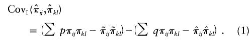The quantity is the difference between the unconditional covariance between the IBD sharing proportions of two pairs of relatives and the conditional covariance of these IBD sharing proportions given the marker genotype data. This difference can be thought of as the information provided by the marker in reducing the level of uncertainty regarding IBD sharing. The fact that the expectation of is equal to the true covariance is shown in appendix B. However, may be negative, seemingly implying that the marker data have increased the uncertainty about IBD sharing. For example, if the posterior probabilities of sharing 0, 1, and 2 alleles IBD for sib pair (i,j) are 0.5, 0, and 0.5, respectively, then the value of is −1/8. Our justification for using despite this curious behavior is that it satisfies the three above properties and appears to result in correct type I error rate in our simulation studies (see below). The matrix of for all pairs of IBD sharing proportions is denoted as .

To give an example of an “imputed covariance matrix,” we consider a sibship of size 3, where sibs 1, 2, and 3 have genotypes AB, AB, and AA, respectively, and the parents are untyped. If the two alleles A and B each have frequency 0.5, then the possible IBD configurations and their prior and posterior probabilities are as given in table 1.

Table 1.

Possible IBD Configurations and Prior and Posterior Probabilities for a Sib Trio with Genotypes AB, AB, and AA, in Which the Two Alleles Have Frequency 0.5

	π for Sib Pair
IBDConfiguration	1-2	1-3	2-3	pa	qb
1	1.0	.0	.0	1/16	1/6
2	.5	.5	.0	1/8	1/6
3	.5	.0	.5	1/8	1/6
4	.0	.5	.5	1/8	1/6
5	1.0	.5	.5	1/8	1/3
6	1.0	1.0	1.0	1/16	0
7	.5	1.0	.5	1/8	0
8	.5	.5	1.0	1/8	0
9	.0	1.0	.0	1/16	0
10	.0	.0	1.0	1/16	0

^ap = prior probability.

^bq = posterior probability.

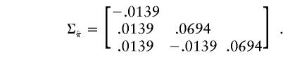
The vector of values of for the three sib pairs, 1-2, 1-3, and 2-3 is (0.67, 0.33, 0.33). By use of equation (1), the “imputed covariance matrix” is calculated as

Covariances between Squared Sums, Squared Differences, and IBD Sharing

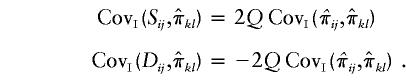
If the phenotypic variance explained by the additive effects of the QTL is Q, then the regression of S_ij on is 2Q (Wright 1997; Drigalenko 1998). The regression of on is . Hence, the regression of S_ij on is , and their covariance is . Similarly, the regression of D_ij on is -2Q (Haseman and Elston 1972), implying that the covariance between S_ij and is .

Because we have only “imputed covariances” between and , we define the required covariances as follows:

These elements define the covariance matrices and , respectively.

Regression of IBD Sharing on Squared Sums and Squared Differences

The proposed method is based on the regression of on S and D. However, for families with four or more individuals, there is collinearity among the elements of S and D. This is because each element is a linear combination of two squares and a cross-product and there are n(n+1)/2 squares and cross-products, whereas there are n(n-1)/2 elements in each of the vectors S and D. For families of size ⩾4, it is clear that there are a greater number of squared sums and squared differences than of their constituent squares and cross-products. To remove this collinearity, we arbitrarily trim the D vector to n elements, such that each individual is represented at least once. Because all the eliminated elements of D are linear combinations of the retained elements of S and D, there is no loss of information. We denote the trimmed vector as d and the corresponding trimmed covariance matrices as Σ_dd, Σ_Sd, and .

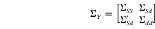
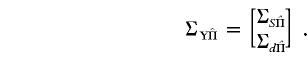
The independent variables S and d are stacked in a single vector . The covariance matrix of Y and the covariance matrix between Y and are the block matrices

and

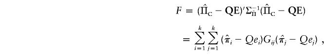
So that the method can be applicable to selected samples, we mean center both the dependent and independent variables around their population means. If the mean-centered vectors are Y_C=Y-E(Y) and , then the multivariate regression equation of on Y_C is

where e is a vector of residuals. The matrix can be factorized into , where Q is a diagonal matrix with diagonal elements Q. Matrix H is composed of two blocks stacked horizontally, where the first block is a square matrix with diagonal elements of 2 and off-diagonal elements of 0 and the second block consists of the first n columns of a similar matrix with diagonals of −2.

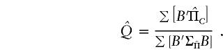
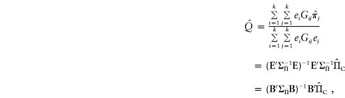
Writing HΣ^-1_YY_C as matrix B, we calculate scalar quantities and . For a given family, the ratio of gives an estimate of Q with sampling variance (see appendix C). Across all pedigrees in a sample, an optimally weighted estimate of Q is given by

Note that these calculations require the inverse of Σ_Y but not the inverse of . By the central limit theorem, a test statistic that in large samples has asymptotically a χ² distribution with 1 df under the null hypothesis is

Since only positive values of Q are biologically meaningful, we adopt a one-tailed test by redefining T as 0 when is negative. The resulting test statistic is distributed as a 50:50 mixture of 0 and χ² with 1 df, under the null hypothesis.

Family Informativeness

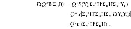
In very large samples, approaches Q, and the test statistic T has expected value

This is the noncentrality parameter (NCP) of the asymptotic noncentral χ² distribution of T. The expected contribution of a family to λ, conditional on the trait values of the family members, and assuming complete marker information, is therefore Q²B^′Σ_ΠB. This index may be used for the selection of informative families for genotyping. It gives values of informativeness similar to those given by another recently proposed index (Purcell et al. 2001), provided that the latter is calculated under a “base model” that assumes equal allele frequencies and additive effects at the QTL.

The expected contribution of a randomly selected family, without knowledge of trait values, is the expected value of Q²B^′Σ_ΠB over all possible trait values:

For general families, there may be no simpler form. However, for sibships, the only parameters in Σ^-1_Y are sibship size s and sib-pair correlation r, and Σ_Π is simply a diagonal matrix with elements Var(π)= 1/8. Although the simplification of this expression is tedious, we have found it to be exactly equivalent to the first non-zero term of the Taylor expansion of the noncentrality parameter of the standard likelihood-ratio test for a QTL in a VC model (appendix D). This turns out to be

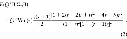For large sibships, this expression gives NCPs that are greater than the corresponding values for VC models. The difference increases with increasing sibship size, as shown in figure 1.

Figure 1.

Theoretical sibship NCP over squared QTL variance Q², obtained from equation (2) for the regression method and from appendix D for the VC method, under the assumption of a sibling correlation of 0.25.

Alternative Specification in Terms of Squares and Cross-Products

An alternative way of removing the collinearity between the squared sums and squared differences is to use the squares and cross-products as independent variables. In other words, the vector of independent variables Y will be the column vector of n(n-1)/2 cross-products and n squares. The trait squares are marginally independent of IBD sharing but do nevertheless explain some variance of IBD sharing jointly with the cross-products. The mean vector of Y, required for mean-centering, will consist of correlations for the cross-products and 1s for the squares. The covariance matrix of Y will be given by the variances and covariances of cross-products and squares, derived by using the formulae in appendix A. The H matrix is then defined as two blocks stacked horizontally, where the first block is an identity matrix of dimension n(n-1)/2 and the second block is a zero matrix of n(n-1)/2 rows and n columns. This alternative specification is equivalent to the one described above, based on all nonredundant squared sums and squared differences, but may have some advantages when the method is generalized to multivariate phenotypes.

Software Implementation

We have combined our new regression-based procedure with the fast pedigree likelihood calculations provided by Merlin (Abecasis et al. 2002). To allow for memory-efficient calculations, our implementation analyzes each pedigree in turn. First, trait squared sums and differences and their covariances are calculated for all family members. Then, the expected allele-sharing scores and imputed covariance matrices are calculated at each position along the chromosome in turn and are used to estimate the contribution of each position to the phenotypic variance. Only one matrix inversion per family is required, and, typically, our method performs much faster than VC analyses.

Our implementation can also conveniently rank families according to their expected informativeness, on the basis of phenotypic values (which can be useful when selecting families to genotype), and can perform gene-dropping simulations for calculation of empirical significance levels. The likelihood calculations required for obtaining IBD sharing probabilities are based on the Lander-Green algorithm and can handle pedigrees of ∼20 individuals for multipoint analysis and ∼30 individuals for single-point analyses. Users must provide a standard pedigree file with normalized trait values, a genetic map for the region of interest, and an estimate of the trait heritability (used for estimation of correlations between relatives).

Simulation Studies

To explore the properties of the new regression-based linkage test and to compare it with the VC method, we conducted a number of simulations. All our simulations share a number of common features. In each data set, we simulated phenotypes for 500 sib-pairs, 333 sets of three siblings (sib-trios), 250 sets of four siblings (sib-quads), or 166 sets of six siblings (sib-hexes), for a total of 1,000 phenotyped individuals in each case. When conducting simulations under the null hypothesis, we examined 20,000 replicate data sets. When examining alternative hypotheses to estimate power, we examined 2,000 replicate data sets in each case. We simulated a diallelic QTL accounting for 0%, 20%, or 50% of the trait variance, with the remaining variance due to additive polygenic effects and random error. In each case, we set the sum of QTL variance and polygenic effects to be 25%, 50%, or 75% of the trait variance. We conducted analyses using either a fully informative marker and parental genotypes, to represent perfect IBD information (a situation that might be approximated with a set of closely spaced microsatellite markers), or genotypes for a diallelic marker with equifrequent alleles and no parental genotypes, to represent imperfect IBD information (an extreme situation of low information that should not be encountered often in practice). Data were analyzed with a new version of Merlin (Abecasis et al. 2002) that implements VC analyses and our new approach.

We first examined whether the method performs correctly under the null hypothesis and provides adequate control of type I error. We varied the overall additive genetic variance from 0.25 to 0.75, arising from either polygenic (normally distributed) effects, an unlinked additive diallelic QTL, or a mixture of the two. Table 2 shows that, under all conditions, the average χ² statistics obtained by use of the regression approach were very near their expected value of 0.5 (since they are 50:50 mixtures of χ²₁ and a point mass of zero), indicating that the expected type I error rate is not biased. As expected, this is also the case for VC analysis. Additionally, the average estimate of Q is zero, indicating a lack of bias. We note that this is not the case for VC, since variance estimates are constrained to be positive. However, this difference is not likely to be of practical importance, since negative estimates of Q from the new method will also be interpreted as 0.

Table 2.

Comparison of Regression and VC Methods under the Null Hypothesis

	Statistic for Hypothesisa
	Perfect Marker				Diallelic Marker
	Regression		VC		Regression		VC
Subjects, Q,and GR	χ2	Q	χ2		χ2		χ2	Q
500 sib pairs:
Q=.00:
.25	.50	.00	.49	.05	.50	−.01	.42	.08
.50	.51	.00	.52	.05	.46	−.02	.50	.09
.75	.50	.00	.50	.04	.44	−.02	.50	.09
Q=.20:
.05	.49	.00	.48	.05	.48	−.01	.41	.08
.30	.49	.00	.50	.05	.45	−.02	.49	.09
.55	.52	.00	.53	.04	.45	−.02	.51	.09
Q=.50:
.00	.50	.00	.52	.05	.45	−.02	.51	.09
.25	.50	.00	.53	.04	.44	−.03	.53	.09
333 sib trios:
Q=.00:
.25	.51	.00	.50	.03	.52	.00	.47	.06
.50	.51	.00	.50	.03	.50	.00	.49	.06
.75	.51	.00	.50	.03	.49	.00	.49	.05
Q=.20:
.05	.49	.00	.48	.03	.50	.00	.46	.06
.30	.51	.00	.50	.03	.51	.00	.50	.06
.55	.51	.00	.50	.03	.50	−.01	.50	.05
Q=.50:
.00	.51	.00	.52	.03	.50	.00	.51	.06
.25	.50	.00	.52	.03	.49	.00	.51	.05
250 sib quads:
Q=.00:
.25	.51	.00	.50	.03	.53	.00	.48	.05
.50	.52	.00	.50	.03	.53	.00	.50	.05
.75	.51	.00	.49	.02	.52	.00	.50	.04
Q=.20:
.05	.52	.00	.50	.03	.55	.00	.50	.05
.30	.51	.00	.49	.03	.50	.00	.48	.04
.55	.51	.00	.49	.02	.50	.00	.48	.04
Q=.50:
.00	.53	.00	.53	.03	.52	.00	.50	.05
.25	.49	.00	.50	.02	.50	.00	.50	.04
166 sib hexes:
Q=.00:
.25	.52	.00	.50	.02	.54	.00	.48	.04
.50	.52	.00	.49	.02	.53	.00	.48	.03
.75	.51	.00	.48	.02	.52	.00	.47	.03
Q=.20:
.05	.51	.00	.49	.02	.52	.00	.47	.04
.30	.51	.00	.49	.02	.55	.00	.50	.03
.55	.52	.00	.50	.02	.55	.00	.50	.03
Q=.50:
.00	.52	.00	.51	.02	.53	.00	.50	.03
.25	.51	.00	.51	.02	.50	.00	.48	.03

^aAverage χ² statistics (χ²) and QTL variance estimates () are based on 20,000 simulated replicates. θ=0.5 in all cases. “Perfect marker” represents complete IBD information; “diallelic marker” has equally frequent alleles. Q and G_R represent QTL and residual polygenic variances, respectively.

We next explored the power of the regression test, for sibships of varying sizes, to detect a QTL explaining either 20% or 50% of the phenotypic variance, while varying the residual polygenic component. As shown in table 3, in the case of sib pairs, power is very similar for the two methods, with perhaps a trivial advantage given to VC. This is the case for both the fully informative marker and the diallelic marker. Estimates of the QTL variance are unbiased in the case of the fully informative marker and are slightly low in the case of the diallelic marker, regardless of the method of analysis. The average χ² statistics from simulations under perfect information agree well with the theoretical values calculated as noncentrality parameter plus 0.5, using equation (2) for the regression method and the equation in appendix D for the VC method (implemented in the Web-based Genetic Power Calculator software).

Table 3.

Comparison of Regression and VC Methods under Various Alternative Hypotheses

	Statistic under Hypothesisa
	Theoretical		Perfect Marker				Diallelic Marker
	Regression	VC	Regression		VC		Regression		VC
Subjects, Q,and GR	χ2	χ2	χ2		χ2		χ2		χ2
500 sib pairs:
Q=.2:
.05	3.12	3.14	3.50	.20	3.29	.18	1.43	.19	1.13	.15
.30	3.52	3.55	4.08	.20	4.14	.20	1.38	.17	1.5	.21
.55	4.36	4.41	4.80	.20	4.93	.20	1.53	.17	1.78	.22
Q=.5:
.00	19.39	20.33	19.25	.49	20.27	.47	4.44	.42	4.8	.41
.25	24.63	26.5	23.93	.48	26.99	.50	4.98	.39	6.23	.48
333 sib trios:
Q=.2:
.05	5.85	5.72	6.42	.20	5.95	.18	2.47	.19	2.07	.16
.30	6.91	6.75	7.31	.20	7.12	.20	2.76	.19	2.66	.20
.55	8.98	8.76	9.37	.20	9.16	.20	3.28	.19	3.26	.20
Q=.5:
.00	40.58	39.78	39.66	.49	39.49	.47	11.74	.46	11.28	.44
.25	53.51	53.39	51.34	.48	53.38	.50	15.03	.45	15.52	.50
250 sib quads:
Q=.2:
.05	8.68	8.24	9.33	.20	8.55	.17	3.83	.20	3.19	.19
.30	10.57	9.99	11.14	.20	10.48	.20	4.34	.20	3.99	.20
.55	14.12	13.27	14.49	.20	13.55	.20	5.45	.20	5.03	.20
Q=.5:
.00	63.43	58.26	61.83	.48	57.81	.45	21.35	.49	18.45	.48
.25	85.62	79.5	82.93	.48	80.39	.50	27.5	.48	24.91	.50
166 sib hexes:
Q=.2:
.05	14.45	12.97	15.21	.20	13.26	.19	6.31	.20	5.06	.18
.30	18.26	16.21	18.98	.20	16.69	.20	7.78	.20	6.54	.20
.55	25.14	21.97	25.82	.20	22.49	.20	10.31	.20	8.53	.20
Q=.5:
.00	111.51	90.73	107.51	.48	90.49	.48	40.89	.51	30.41	.46
.25	154.51	125.4	141.65	.46	124.07	.50	53.25	.48	40.37	.49

^aTheoretical χ² statistics were obtained analytically from equation (2) for the regression method and from appendix D for the VC method. Average χ² statistics and were obtained from 2,000 simulated replicates. θ=0 in all cases. Q and G_R represent QTL and residual polygenic variances, respectively. “Perfect marker” represents complete IBD information; “diallelic marker” has equally frequent alleles.

When examining progressively larger sibships, we see the regression approach showing greater power than VC, and, for sibships of size 6, this can be as large as a 30% increase in the estimated noncentrality parameter. This difference appears more pronounced when we analyze the less informative diallelic marker, although is still quite apparent in the case of complete information.

Table 4 shows the results of simulations conducted to explore the properties of the regression method when selected samples of various types are analyzed. VC was not compared, since it is known to be liberal when applied to selected samples (Dolan et al. 1999). In all cases, the QTL and polygenic effects explained 20% and 30% of the total variance, respectively. For each replicate, 10,000 phenotyped individuals were simulated, with 10% of the sample selected for analysis. Three different types of selection were explored: (1) affected sibships (ASP), where at least two members of the sibship were required to score above a certain threshold, (2) discordant sibship (DSP), where at least one member of the sibship was required to score above a chosen threshold and another below a chosen threshold, and (3) the most informative sibships, selected according to the criterion B^′Σ_ΠB as described above. Under the null case of no linkage to the trait locus (recombination fraction [θ] 0.5), the average χ² is, in all cases, very close to its expected value of 0.5, and Q is correctly estimated at zero. Under the case of linkage, the regression method appears to be performing correctly, recovering 55% of the full-sample χ² with the most-informative 10% of sib pairs and a fully informative marker. The method also estimates the QTL variance without any noticeable bias in all cases.

Table 4.

Average χ² Statistics of the Regression Method in Selected Samples

	Statistic under Hypothesisa
	Perfect Marker					Diallelic Marker
	θ=0.5		θ=0.0			θ=0.5		θ=0.0
Families and Selection Strategy	χ2		χ2		Efficiency(%)	χ2		χ2		Efficiency(%)
500/5,000 sib pairs:
Random	.49	.00	4.08	.20	10	.45	−.02	1.38	.17	10
ASP	.50	.00	4.46	.17	11	.57	−.02	2.06	.21	15
DSP	.49	.00	19.69	.22	48	.46	−.01	4.30	.18	31
INF	.50	.00	22.62	.20	55	.47	−.01	5.36	.18	39
333/3,330 sib trios:
Random	.51	.00	7.31	.20	10	.51	.00	2.76	.19	10
ASP	.51	.00	14.70	.20	20	.52	.00	5.11	.20	19
DSP	.50	.00	29.27	.20	40	.49	.00	8.80	.19	32
INF	.51	.00	37.04	.20	51	.48	.00	11.07	.19	40
250/2,500 sib quads:
Random	.51	.00	11.14	.20	10	.50	.00	4.34	.20	10
ASP	.52	.00	22.17	.19	20	.52	.00	8.22	.20	19
DSP	.50	.00	42.31	.21	38	.50	.00	13.92	.20	32
INF	.50	.00	52.05	.20	47	.50	.00	17.02	.20	39

^aAverage χ² statistics and obtained from 20,000 simulated replicates for θ=0.5, and 2,000 simulated replicates for θ=0.0. In each case, Q = 0.2, G_R = 0.3, and 10% of the simulated sample is selected for analysis. The ASP, DSP, and INF methods of selection correspond to affected sib pairs, discordant sib pairs, and information index (see text), respectively. “Perfect marker” represents complete IBD information; “diallelic marker” has equally frequent alleles. Efficiency is calculated as the ratio of the average χ² statistic of each selection scheme to that of the entire sample.

We next evaluated the performance of the regression method when analyzing a non-normally distributed trait. The trait was simulated as before, and the trait values of each family were divided by a χ² random variable with 12 df. This transforms a multivariate normal distribution to a markedly leptokurtic multivariate t distribution. Outliers >3 SD away from the mean were winsorized to exactly 3 SD from the mean. Table 5 shows that with a fully informative marker, the regression method has the correct type I error rate, as evidenced by the average χ² statistics of ∼0.5, whereas the VC method consistently produces inflated average χ² statistics, in the range 0.7–0.8, as shown in table 6. However, in the case of the diallelic marker with low information, the regression method does show an increased type I error rate. This is shown by both the inflated average χ² statistics and the significant proportions of replicates that exceed the 0.01 critical value. This liberal behavior can also be seen in examination of the linked case, where the test appears to be more powerful for the diallelic marker than for the perfectly informative marker, in the case of the larger sibships and a QTL explaining 50% of trait variance. We have shown, by further simulation studies, that the liberal behavior of the regression method, in the case of poor marker information, is reduced as the number of pedigrees increases. For the case where the QTL and residual polygenes account for 50% and 25% of trait variance, respectively, the average χ² statistics for 250, 500, 1,000, and 2,000 sibships of size 4 are 1.180, 0.705, 0.628, and 0.545, respectively. For the VC method, similar simulations of larger sample sizes show that the average χ² statistics remain inflated, in the range 0.7–0.8. Comparing the fully informative case to the comparable situation in table 3, we see that power is lost when analyzing this extremely non-normally distributed trait, but it is still possible to detect the QTL if an informative marker situation is available, as would be the case in a multipoint analysis using microsatellite markers.

Table 5.

Average χ² Statistics of the Regression Method in Non-Normal Samples

	Statistic under Hypothesisa
	θ=0.5						θ=0.0
	Perfect Marker			Diallelic Marker			Perfect Marker		Diallelic Marker
Subjects, Q,and GR	χ2	α.01		χ2	α.01		χ2		χ2
500 sib pairs:
Q=.00:
.25	.50	.009	.00	.57	.017	.02	…	…	…	…
.50	.51	.009	.00	.63	.019	.03	…	…	…	…
.75	.50	.009	.00	.69	.027	.04	…	…	…	…
Q=.20:
.05	.50	.010	.00	.55	.014	.01	2.58	.14	1.28	.15
.30	.50	.008	.00	.64	.021	.03	2.57	.13	1.43	.16
.55	.49	.009	.00	.66	.023	.03	2.39	.12	1.52	.17
Q=.50:
.00	.49	.009	.00	.62	.020	.03	10.82	.33	3.93	.39
.25	.49	.009	.00	.65	.023	.03	10.10	.30	4.04	.38
250 sib quads:
Q=.00:
.25	.51	.012	.00	.60	.021	.01	…	…	…	…
.50	.52	.011	.00	.81	.028	.04	…	…	…	…
.75	.52	.012	.00	1.54	.037	.09	…	…	…	…
Q=.20:
.05	.52	.012	.00	.60	.021	.01	6.14	.14	3.03	.17
.30	.52	.012	.00	.73	.027	.01	6.01	.14	3.83	.22
.55	.51	.013	.00	1.77	.038	.08	5.46	.12	5.22	.25
Q=.50:
.00	.53	.013	.00	.71	.023	.02	33.60	.35	17.43	.48
.25	.53	.013	.00	1.18	.035	.05	29.76	.31	38.14	1.01

^aAverage χ² statistics, empirical α_.01 levels, and obtained from 20,000 simulated replicates for θ=0.5, and 2,000 simulated replicates for θ=0.0. In each case, the trait values of sibships have been transformed to a multivariate t distribution with 12 df, to simulate a leptokurtic distribution. Q and G_R represent QTL and residual polygenic variances, respectively. “Perfect marker” represents complete IBD information; “diallelic marker” has equally frequent alleles.

Table 6.

Average χ² Statistics of the VC Method in Non-Normal Samples

	Statistic under Hypothesisa
	θ=0.5				θ=0.0
	Perfect Marker		Diallelic Marker		Perfect Marker		Diallelic Marker
Subjects, Q,and GR	χ2		χ2		χ2		χ2
500 sib pairs:
Q=.00:
.25	.697	.055	.549	.086	…	…	…	…
.50	.752	.057	.726	.110	…	…	…	…
.75	.785	.051	.781	.106	…	…	…	…
Q=.20:
.05	.711	.056	.548	.085	1.830	.213	1.258	.150
.30	.780	.058	.721	.110	4.640	.206	3.460	.166
.55	.817	.053	.765	.105	5.276	.200	2.156	.228
Q=.50:
.00	.791	.058	.743	.111	20.166	.452	5.124	.392
.25	.831	.053	.819	.045	27.774	.500	6.821	.470
250 sib quads:
Q=.00:
.25	.709	.033	.661	.055	…	…	…	…
.50	.727	.031	.709	.054	…	…	…	…
.75	.739	.027	.717	.046	…	…	…	…
Q=.20:
.05	.714	.033	.666	.055	8.765	.181	3.395	.165
.30	.718	.031	.692	.053	10.999	.201	4.465	.203
.55	.712	.026	.697	.046	14.387	.202	5.556	.203
Q=.50:
.00	.748	.031	.721	.054	24.810	.492	18.579	.446
.25	.783	.028	.752	.047	80.226	.500	59.055	.472

^aAverage χ² statistics and H², obtained from 20,000 simulated replicates for θ=0.5, and 2,000 simulated replicates for θ=0.0. In each case, the trait values of sibships have been transformed to a multivariate t distribution with 12 df, to simulate a leptokurtic distribution. Q and G_R represent QTL and residual polygenic variances, respectively. “Perfect marker” represents complete IBD information; diallelic marker has equally frequent alleles.

Next, we explored the robustness of our regression method to misspecification of population mean, variance, and correlation, as shown in figure 2. In an unselected sample of 250 sibships of size 4, we simulated a QTL explaining 20% of the variance, with polygenic variance set at 30%, as was done for table 4. The trait was simulated to have a mean of 0 and a variance of 1. To test the robustness of the method to misspecification, in both the unlinked and linked cases, in panel a, we fixed the mean to a range of values from −1 to 1, including the true value 0. In the unlinked case, we detected a small bias in the average χ² when analyzing the diallelic marker, although no suggestion of increased type I error results in the fully informative case. Misspecification of the variance (panel b) from 0.5 to 2 also appears to have little impact on type I error rate. However, fixing the heritability at 0 (panel c) does result in a slight increase in type I errors in the case of a diallelic marker. Fixing the heritability at 1 does not have such an effect. Turning to the issue of power under misspecification (the curves representing the alternate hypotheses), it appears that misspecification of the mean can have a nontrivial impact, reducing power considerably. However, we do not see such a large effect for the variance or the heritability.

Figure 2.

Effect of model misspecification. Each point represents the average χ² statistic obtained from 2,000 simulated replicates, containing 250 sib quads. The QTL and residual polygenic variances are 0.2 and 0.3, respectively. In each case, the true trait model has mean 0, variance 1, and heritability 0.5. The misspecified mean, variance, and covariance are shown on the X-axes of panels a, b, and c, respectively. “Perfect marker” represents complete IBD information; “imperfect marker” represents a diallelic marker with equally frequent alleles.

Thus far, we have explored only sibship data. However, the method is applicable to general pedigrees of all types. Our last set of simulations deals with the case of cousin pedigrees, where each pedigree contains 10 individuals, comprising a set of two grandparents and their four grandchildren distributed in two sibships of size 2 (see fig. 3). We simulated 200 pedigrees per replicate and compared the performance of our regression approach with VC in table 7. In the unlinked case, there is little suggestion of bias in type I error rate for the regression method, as can be seen from all average χ² values being very close to their expected value of 0.5 for the fully informative case and showing only a hint of inflated type I for the uninformative diallelic marker. Average χ² statistics are also extremely close to their expected value of 0.5 for VC.

Figure 3.

Structure for simulated cousin pedigree

Table 7.

Average χ² Statistics of the Regression and VC Methods for Cousin Pedigrees

	Statistic for Hypothesisa
	Perfect Marker				Diallelic Marker
	Regression		VC		Regression		VC
θ, Q, andGR for 200CousinPedigrees	χ2		χ2		χ2		χ2
θ.=5:
Q=.00:
.25	.51	.00	.50	.02	.54	.00	.50	.05
.50	.51	.00	.50	.02	.54	.00	.51	.04
.75	.53	.00	.51	.02	.55	.00	.51	.04
Q=.20:
.05	.52	.00	.51	.03	.53	.00	.49	.05
.30	.49	.00	.48	.03	.53	.00	.50	.04
.55	.50	.00	.49	.02	.53	.00	.50	.04
Q=.50:
.00	.52	.00	.52	.02	.53	.00	.51	.04
.25	.51	.00	.52	.02	.53	.00	.51	.04
θ=.0:
Q=.20:
.05	4.45	.21	3.76	.18	11.75	.20	11.02	.19
.30	4.94	.21	4.43	.20	13.21	.20	12.56	.20
.55	6.26	.22	5.56	.20	16.80	.20	15.95	.20
Q=.50:
.00	26.00	.56	21.24	.46	73.85	.49	71.42	.48
.25	33.94	.56	28.27	.50	93.68	.48	93.41	.50

^aAverage χ² statistics and obtained from 20,000 replicates for θ=0.5 and 2,000 simulated for θ=0.0. Each replicate has 200 three-generation pedigrees (see fig. 3). Q and G_R represent QTL and residual polygenic variances, respectively. “Perfect marker” represents complete IBD information; “diallelic marker” has equally frequent alleles.

In the linked case, it appears the regression method is again slightly more powerful than VC, for the fully informative marker case. This is also somewhat true for the diallelic marker, although the small difference in power may in fact be attributable to the slightly inflated type I error rate. However, such bias was not seen for the fully informative case, suggesting that the increased power is, in fact, real.

Discussion

Several methods are currently available for QTL linkage analysis, but none is entirely satisfactory. The penetrance-based method requires the specification of allele frequencies, genotype-specific trait means, and the residual covariance structure (Hasstedt 1994). This method assumes multivariate normality conditional on QTL genotype and is computationally intensive for large pedigrees. Moreover, power is optimal only when the true QTL model is diallelic, and it may be substantially reduced when the underlying QTL has multiple alleles of variable effects (Goring et al. 2001).

The VC method (Hopper and Matthews 1982; Schork 1993; Amos 1994; Eaves et al. 1996; Fulker and Cherny 1996; Almasy and Blangero 1998) specifies the covariances between relatives as a function of the proportion of alleles IBD (π) at the putative QTL. This method assumes multivariate normality conditional on IBD sharing and produces liberal P values when applied to samples selected for phenotypic extremes (Dolan et al. 1999). Robustness to phenotypic selection can be achieved by conditioning on trait values (Sham et al. 2000b), but this is computationally intensive in large pedigrees because of the need to invert the implied covariance matrices of all possible inheritance vectors. Score tests from the VC model have been recently derived (Putter et al. 2002; Wang and Huang 2002), but the properties of these tests in phenotypically selected samples have yet to be examined.

Regression-based methods (Wright 1997; Drigalenko 1998; Elston et al. 2000; Xu et al. 2000; Forrest 2001; Sham and Purcell 2001) have been shown to have power equivalent to that of VC models for sib pairs (Sham and Purcell 2001). Attempts have been made to extend the regression approach to sibships but not to general pedigrees (Elston et al. 2000). Similarly, although composite statistics have been proposed to enhance the power of regression-based methods in phenotypically selected samples (Forrest and Feingold 2000), this has yet to be extended to general pedigrees.

The proposed regression-based method combines the advantages of existing methods: (1) it is conceptually and computationally simple; (2) it is applicable to general pedigrees; (3) it provides an estimate of the proportion of variance accounted for by the QTL; (4) it provides a test of linkage that is asymptotically χ²; (5) it makes appropriate use of incomplete IBD information; (6) it is applicable to samples selected for phenotypic extremes, provided that approximate values of the population mean, variance, and correlations (between relatives) can be specified; and (7) it leads naturally to a simple measure of family informativeness. In addition, the new test has slightly greater power than VC in large sibships. Some of these desirable properties follow directly from the way that the method is constructed; others have been established by the simulation studies reported above.

The noncentrality parameter of the proposed regression method is equivalent to the second-order term of the Taylor expansion of the VC likelihood-ratio test, at least for the case of sibships. This suggests that our regression-based method is closely related to the score test of the VC model. It is somewhat surprising that the regression test is more powerful than VC; this is due to higher-order terms in the VC likelihood-ratio test. Such terms may be particularly prominent in sibship data, because for sibships of size ⩾3, IBD sharing is pairwise independent but not jointly independent (Hodge 1984; Blackwelder and Elston 1985). Recently, Wang and Huang (2002) and Putter et al. (2002) have independently derived score tests from the VC model; both have shown the modified H-E method of Sham and Purcell (2001) to be a special case of their tests. It is unclear whether these methods can be directly applied to selected samples. Our proposed regression-based method is applicable to selected samples and, furthermore, provides an estimate of the proportion of variance explained by the additive effects of the QTL.

The treatment of incomplete marker information by the use of “imputed covariances” of IBD sharing is another novel feature. Other authors have suggested the use of sample estimates of variances and covariances of IBD sharing (Dudoit and Speed 2000; Wang and Huang 2002). This has the disadvantage that sample estimates may be inaccurate if only a small number of pedigrees of a certain configuration are present in the sample. Furthermore, sample variances and covariances of IBD sharing may be different from their respective population values for phenotypically selected samples and therefore are likely to result in lower power. The use of an “imputed covariance” that can be calculated from the joint IBD probabilities for two relative pairs appears to be simple and effective in our simulations. However, we have not shown that the proposed definition for “imputed covariance” is the only suitable one, and it may be possible to find alternative definitions that are equally appropriate. One interesting alternative definition for the “imputed covariance” is , which satisfies the last two properties that we considered desirable, but not the first one.

One problem with the proposed method is that it can be liberal in some circumstances, as is shown in the simulations. Since the test relies on the central limit theorem for its asymptotic distribution, liberal significance levels can result from a combination of two factors: (1) a small number of families contributing to the test statistic and (2) highly skewed contributions from some families. Low marker informativeness can reduce the effective number of contributing families, whereas a highly leptokurtic trait distribution can lead to highly skewed contributions from some pedigrees with extreme scores. The combination of these two factors is why our simulations revealed an inflated type I error rate for the situation where a highly leptokurtic trait is coupled with an uninformative marker. In practice, multipoint analysis should provide almost complete IBD information. Furthermore, any apparent non-normality in the data should have been minimized by a normalizing transformation. An additional safeguard against outlying observations that persist after transformation is winsorization; any observations that are ⩾k SD from the mean are recoded to precisely k SD from the mean (for a reasonable choice of k). If these precautions are taken and the sample consists of a reasonably large number of families, then the test we propose based on the χ² distribution should provide very accurate P values. Nevertheless, it should be straightforward to verify significance levels for any interesting findings by using Monte Carlo methods (such as gene-dropping simulations). Since our method is based on linear regression, it is ideally suited to these empirical analyses.

The proposed regression-based method provides a practical and powerful tool for the linkage analysis of quantitative traits. At present, the method is limited to additive genetic effects on a single quantitative trait. However, it has the potential to be extended to include dominance and epistatic effects, qualitative traits, and multiple phenotypes.

Appendix A: Covariances of Squared Sums and Squared Differences

If X_i, X_j, X_k, and X_l are multivariate normal with means 0 and variance 1, then, from Mardia et al. (1979, p. 95), it can be shown that

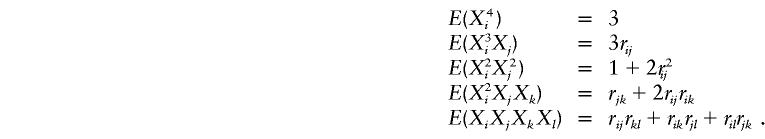These expressions are used to obtain

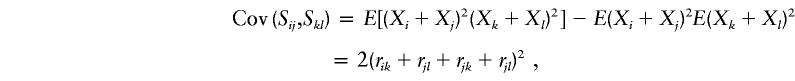and similarly for Cov(S_ij,D_kl) and Cov(D_ij,D_kl).

Appendix B : Expectation of “Imputed Covariances” of IBD Sharing

The expectation of the “imputed covariance” of estimated IBD sharing proportions is

The expectation of π_ijπ_kl conditional on a family’s genotype combination over all possible genotype combinations is equal to unconditional expectation of π_ijπ_kl. Furthermore, . Therefore,

Appendix C : Estimation of

We wish to minimize

Define as the vector E, then

where G_ij is element (i,j) of . Differentiating with respect to Q and equating to 0, we obtain

Hence,

with variance

Appendix D : Taylor Expansion of Noncentrality Parameter of Likelihood-Ratio Test

We have shown elsewhere (Sham et al. 2000a) that the NCP for the linkage test in the VC model is λ=-E(ln|Σ_π|)+ln|Σ₀|, where Σ_π is the covariance matrix conditional on a pattern of IBD sharing π, and Σ₀ is Σ_π evaluated at the expected values of π (e.g., 0.5 for sib pairs).

The expectation can be expanded around the expected values of π as follows:

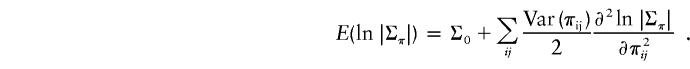There are no terms involving first-order derivatives, because expected deviations from the mean are 0. For sibships, the covariance between any two πs is 0, so that the second-order terms involve only the variances of π. By symmetry, we need only consider one particular pair, say π₁₂. Treating π₁₂ as variable and fixing all other π’s at their expected values, it can be shown that |Σ_π| is

where π_C is the mean-centered value of π₁₂. Differentiating this twice and setting π_c to zero, we obtain

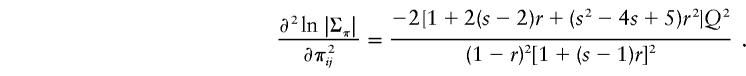There are s(s-1)/2 possible sib pairs, each making an equal contribution, and so the NCP is approximated to the second order by equation (2).

References

- Abecasis GR, Cherny SS, Cookson WO, Cardon LR (2002) Merlin—rapid analysis of dense genetic maps using sparse gene flow trees. Nat Genet 30:97–101 [DOI] [PubMed] [Google Scholar]
- Allison DB, Fernandez JR, Heo M, Beasley TM (2000) Testing the robustness of the new Haseman-Elston quantitative-trait loci-mapping procedure. Am J Hum Genet 67:249–252 [DOI] [PMC free article] [PubMed] [Google Scholar]
- Almasy L, Blangero J (1998) Multipoint quantitative-trait linkage analysis in general pedigrees. Am J Hum Genet 62:1198–1211 [DOI] [PMC free article] [PubMed] [Google Scholar]
- Amos CI (1994) Robust variance-components approach for assessing genetic linkage in pedigrees. Am J Hum Genet 54:535–543 [PMC free article] [PubMed] [Google Scholar]
- Blackwelder WC, Elston RC (1985) A comparison of sib-pair linkage tests for disease susceptibility loci. Genet Epidemiol 2:85–97 [DOI] [PubMed] [Google Scholar]
- Chatziplis DG, Hamann H, Haley CS (2001) Selection and subsequent analysis of sib pair data for QTL detection. Genet Res 78:177–186 [DOI] [PubMed] [Google Scholar]
- Curtis D, Sham PC (1994) Using risk calculation to implement an extended relative pair analysis. Ann Hum Genet 58:151–162 [DOI] [PubMed] [Google Scholar]
- Dolan CV, Boomsma DI, Neale MC (1999) A simulation study of the effects of assignment of prior identity-by-descent probabilities to unselected sib pairs, in covariance-structure modeling of a quantitative-trait locus. Am J Hum Genet 64:268–280 [DOI] [PMC free article] [PubMed] [Google Scholar]
- Drigalenko E (1998) How sib pairs reveal linkage. Am J Hum Genet 63:1242–1245 [PMC free article] [PubMed] [Google Scholar]
- Dudoit S, Speed TP (2000) A score test for the linkage analysis of qualitative and quantitative traits based on identity by descent data from sib-pairs. Biostatistics 1:1–26 [DOI] [PubMed] [Google Scholar]
- Eaves LJ, Neale MC, Maes H (1996) Multivariate multipoint linkage analysis of quantitative trait loci. Behav Genet 26:519–525 [DOI] [PubMed] [Google Scholar]
- Elston RC, Buxbaum S, Jacobs KB, Olson JM (2000) Haseman and Elston revisited. Genet Epidemiol 19:1–17 [DOI] [PubMed] [Google Scholar]
- Elston RC, Stewart J (1971) A general model for the analysis of pedigree data. Hum Hered 21:523–542 [DOI] [PubMed] [Google Scholar]
- Feingold E (2001) Methods for linkage analysis of quantitative trait loci in humans. Theor Popul Biol 60:167–180 [DOI] [PubMed] [Google Scholar]
- Forrest W (2001) Weighting improves the “new Haseman-Elston” method. Hum Hered 52:47–54 [DOI] [PubMed] [Google Scholar]
- Forrest W, Feingold E (2000) Composite statistics for QTL mapping with moderately discordant sibling pairs. Am J Hum Genet 66:1642–1660 [DOI] [PMC free article] [PubMed] [Google Scholar]
- Fulker DW, Cherny SS (1996) An improved multipoint sib-pair analysis of quantitative traits. Behav Genet 26:527–532 [DOI] [PubMed] [Google Scholar]
- Goring H, Williams J, Blangero J (2001) Linkage analysis of quantitative traits in randomly ascertained pedigrees: comparison of penetrance-based and variance component analysis. Genet Epidemiol 21:S783–S788 [DOI] [PubMed] [Google Scholar]
- Gudbjartsson D, Jonasson K, Frigge M, Kong A (2000) Allegro, a new computer program for multipoint linkage analysis. Nat Genet 25:12–13 [DOI] [PubMed] [Google Scholar]
- Haseman JK, Elston RC (1972) The investigation of linkage between a quantitative trait and a marker locus. Behav Genet 2:3–19 [DOI] [PubMed] [Google Scholar]
- Hasstedt SJ (1994) PAP: pedigree analysis package. Rev. 4. Department of Human Genetics, University of Utah, Salt Lake City [Google Scholar]
- Heath SC (1997) Markov chain Monte Carlo segregation and linkage analysis for oligogenic models. Am J Hum Genet 61:748–760 [DOI] [PMC free article] [PubMed] [Google Scholar]
- Henshall JM, Goddard ME (1999) Multiple-trait mapping of quantitative trait loci after selective genotyping using logistic regression. Genetics 151:885–894 [DOI] [PMC free article] [PubMed] [Google Scholar]
- Hodge SE (1984) The information contained in multiple sibling pairs. Genet Epidemiol 1:109–122 [DOI] [PubMed] [Google Scholar]
- Hopper JL, Matthews JD (1982) Extensions to multivariate normal models for pedigree analysis. Ann Hum Genet 46:373–383 [DOI] [PubMed] [Google Scholar]
- Kruglyak L, Daly MJ, Reeve-Daly MP, Lander ES (1996) Parametric and nonparametric linkage analysis: a unified multipoint approach. Am J Hum Genet 58:1347–1363 [PMC free article] [PubMed] [Google Scholar]
- Lander ES, Green P (1987) Construction of multilocus genetic maps in humans. Proc Natl Acad Sci USA 84:2363–2367 [DOI] [PMC free article] [PubMed] [Google Scholar]
- Mardia KV, Kent JT, Bibby JM (1979) Multivariate analysis. Academic Press, London [Google Scholar]
- Purcell S, Cherny S, Hewitt J, Sham P (2001) Optimal sibship selection for genotyping in quantitative trait locus linkage analysis. Hum Hered 52:1–13 [DOI] [PubMed] [Google Scholar]
- Putter H, Sandkuijl LA, van Houwelinegen JC (2002) A score test for detecting linkage to quantitative traits. Genet Epidemiol 22:345–355 [DOI] [PubMed] [Google Scholar]
- Schork NJ (1993) Extended multipoint identity-by-descent analysis of human quantitative traits: efficiency, power, and modeling considerations. Am J Hum Genet 53:1306–1319 [PMC free article] [PubMed] [Google Scholar]
- Sham PC, Cherny SS, Purcell S, Hewitt JK (2000a) Power of linkage versus association analysis of quantitative traits, by use of variance-components models, for sibship data. Am J Hum Genet 66:1616–1630 [DOI] [PMC free article] [PubMed] [Google Scholar]
- Sham PC, Purcell S (2001) Equivalence between Haseman-Elston and variance-components linkage analyses for sib pairs. Am J Hum Genet 68:1527–1532 [DOI] [PMC free article] [PubMed] [Google Scholar]
- Sham PC, Zhao JH, Cherny S, Hewitt J (2000b) Variance-components QTL linkage analysis of selected and non-normal samples: conditioning on trait values. Genet Epidemiol 19:S22–S28 [DOI] [PubMed] [Google Scholar]
- Sobel E, Sengul H, Weeks DE (2001) Multipoint estimation of IBD probabilities at arbitrary positions among marker loci on general pedigrees. Hum Hered 52:121–131 [DOI] [PubMed] [Google Scholar]
- Thompson EA (2000) MCMC estimation of multilocus genome sharing and multipoint gene location scores. Int Stat Rev 68:53–73 [Google Scholar]
- Visscher PM, Hopper JL (2001) Power of regression and maximum likelihood methods to map QTL from sib-pair and DZ twin data. Ann Hum Genet 65:583–601 [DOI] [PubMed] [Google Scholar]
- Wang K, Huang J (2002) A score-statistic approach for the mapping of quantitative-trait loci with sibships of arbitrary size. Am J Hum Genet 70:412–424 [DOI] [PMC free article] [PubMed] [Google Scholar]
- Wright FA (1997) The phenotypic difference discards sib-pair QTL linkage information. Am J Hum Genet 60:740–742 [PMC free article] [PubMed] [Google Scholar]
- Xu X, Weiss S, Xu X, Wei LJ (2000) A unified Haseman-Elston method for testing linkage with quantitative traits. Am J Hum Genet 67:1025–1028 [DOI] [PMC free article] [PubMed] [Google Scholar]