Simultaneous modeling of visual saliency and value computation improves predictions of economic choice

Significance

Many everyday decisions require viewing displays with several alternatives and then rapidly choosing one, e.g., choosing a snack from a vending machine. Each item has objective visual properties, such as saliency, and subjective properties, such as value. Objective and subjective properties are usually studied independently. We have implemented a single integrated paradigm that links perceptual with economic decision making by having subjects search through visual displays to choose a single food item that they want to eat. We demonstrate that two linked accumulator models, one modeling perceptual and the other modeling economic decisions, account for subjects’ viewing patterns and choices.

Abstract

Many decisions we make require visually identifying and evaluating numerous alternatives quickly. These usually vary in reward, or value, and in low-level visual properties, such as saliency. Both saliency and value influence the final decision. In particular, saliency affects fixation locations and durations, which are predictive of choices. However, it is unknown how saliency propagates to the final decision. Moreover, the relative influence of saliency and value is unclear. Here we address these questions with an integrated model that combines a perceptual decision process about where and when to look with an economic decision process about what to choose. The perceptual decision process is modeled as a drift–diffusion model (DDM) process for each alternative. Using psychophysical data from a multiple-alternative, forced-choice task, in which subjects have to pick one food item from a crowded display via eye movements, we test four models where each DDM process is driven by (i) saliency or (ii) value alone or (iii) an additive or (iv) a multiplicative combination of both. We find that models including both saliency and value weighted in a one-third to two-thirds ratio (saliency-to-value) significantly outperform models based on either quantity alone. These eye fixation patterns modulate an economic decision process, also described as a DDM process driven by value. Our combined model quantitatively explains fixation patterns and choices with similar or better accuracy than previous models, suggesting that visual saliency has a smaller, but significant, influence than value and that saliency affects choices indirectly through perceptual decisions that modulate economic decisions.

One important goal of neuroscience and economics is to understand the computational mechanisms that underlie decision making between multiple alternatives. Interestingly, this goal has proceeded along two seemingly parallel paths that consider either perceptual decision making, namely decisions about perceptual properties of alternatives, or economic decision making, which considers the value of alternatives (1). Although these types of decisions can be constructed to be mutually exclusive in the laboratory, in more natural contexts, decisions nearly always involve perceptual decisions about how to sample information and value-based decisions about which alternatives are more valuable. Importantly, however, very little attention has been paid to how perceptual and economic decision processes may interact. One recent paper reported a visual saliency bias where, independent of consumer preferences, visually salient options are more likely to be chosen than less salient alternatives. It is not clear, however, which mechanism gives rise to this effect or how perceptual processes interact with economic choices (2).

Choices and reaction times during perceptual decision making have been accurately modeled by stochastic accumulator models such as the drift–diffusion model (DDM) (3), the race model (4), and the leaky competing accumulator model (LCA) (5). Such accumulator models also quantitatively model economic choices in a wide array of tasks (6–9).

These models assume that noisy evidence is accumulated over time and that decisions are made by comparing the evidence between each alternative. When the relative evidence for one option exceeds a threshold, that option is chosen. In perceptual decision-making tasks, the noise typically comes from the stimulus itself, e.g., in moving-dot experiments where the noise is set by the dots’ movement coherence (cf. ref. 10). In economic decision-maki2ng tasks, the noise can come from several sources including shifts in attention between alternatives or sampling (11, 12).

Eye movements are considered a good measure of overt attention (13, 14) and recent work has used eye movements as a measure of the shifts in attention that influence economic decisions. This model [the attentional DDM (aDDM)] has been shown to accurately model choices and mean reaction times in two- and three-alternative economic decisions (6, 8, 9). This model clearly shows how fixation durations and fixation sequences affect choices. However, in these studies, fixations were always measured empirically and then used as input to their model, thus “taking the fixation process as exogenously given” (ref. 9, p. 2).

Meanwhile, decades of research in visual neuroscience have yielded numerous models of the fixation process in many different tasks, including free viewing (cf. ref. 15), reading (cf. ref. 16), and visual search (cf. ref. 17). In economic decision tasks between simultaneously presented alternatives, the task resembles a multiple-target visual search. Eye movements during visual search are generally assumed to be the result of a winner-take-all process operating on an underlying saliency map (17–21). The saliency map can include exogenous, physical conspicuity (“bottom–up” saliency) and/or intrinsic or behavioral relevance (“top–down” information) (21). By assuming that the observer’s gaze transitions between regions of high saliency, these models accurately predict fixation locations with up to 90% accuracy (22, 23).

Accumulator models also account for saccade target selection and time to saccade (or reaction time) in tasks where monkeys make single saccades from a central fixation point to a chosen stimulus (24, 25). Such models are particularly attractive for this task because, in addition to quantitatively explaining the psychometrics and reaction times during perceptual choice, they have a neurally plausible implementation. Specifically, visually responsive neurons in the frontal eye fields (FEFs) change their firing rates in response to both bottom–up saliency and top–down goals (26–31). These neurons drive the firing rates of the FEFs and superior colliculus (SC) movement neurons, which behave like stochastic integrators by increasing their firing rates to a fixed threshold and then initiating a saccade via the oculomotor brainstem nuclei (24, 32–36). However, most of these studies consider only one decision per trial (e.g., the first saccade) and allow the decision process to reset between trials. Although this type of task allows clean modeling of target selection and reaction times, it does not necessarily generalize to tasks where subjects are allowed to overtly search a display through multiple, sequential eye movements.

One recent paradigm for studying decisions during multiple-target search involves subjects searching an array of food items for an item they would like to eat (cf. ref. 8). These decisions involve a combination of perceptual decision making about where to move the eyes and economic decision making about which alternative to choose. We present a model assuming two parallel processes are involved in visual search for a liked item. One process evaluates an item’s value as it is being viewed whereas the other process determines where the eyes will go next. The former we expect is influenced explicitly by value and implicitly by saliency. The latter we expect is explicitly influenced by both saliency and value (cf. refs. 37 and 38). The model is tested with eye-tracking and psychophysical data from subjects performing a search task for a liked food item.

Our combined model of perceptual and economic decision making, validated with an eye-tracking experiment, addresses the following questions. First, to what extent can stochastic accumulator models account for the fixation locations, durations, and sequences in an economic visual search task? Second, to what extent do bottom–up saliency and top–down value influence choices? And, third, can parallel perceptual and economic decision-making processes account for fixations and choices during behaviorally relevant decision making?

Computational Model

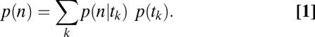
Ultimately, we want to model the probability that subjects will choose a particular item n, which we denote . We decomposed this problem into two simpler pieces, using the law of total probability (Eq. 1). This allows us to model the probability that a subject’s gaze will follow a certain trajectory, , and the conditional probability that a subject chose item n given that his/her gaze followed a certain trajectory, , separately. We call the model of the “gaze model” and the model of the “conditional choice model”:

The Gaze Model of .

To model the gaze trajectory, , we assume that each fixation location is the outcome of a decision about the next fixation location. We model this decision process using the DDM, assuming that each fixation location has a DDM unit driven by a weighted combination of saliency and value. By solving for the first passage times, we calculate the probability that gaze will transition from one fixation location to another, , and the probability of the transition time, .

The DDM.

The drift–diffusion model has been widely used to model decision making (3, 10, 39–41) and saccadic target selection in single-saccade paradigms (24, 25). It can be formulated as shown in Eq. 2, where is the variable that is accumulating, is the drift of the jth accumulator, t is time, c is the SD of zero-mean Gaussian-distributed noise, and is a Wiener process:

Here, the drift is either the sum or the product of saliency and value with normalized weights and , respectively:

In the single alternative DDM, noisy evidence accumulates to a specific threshold, θ, whereupon a decision is made. When there are multiple alternatives and one accumulator for each alternative, the first accumulator to reach the threshold indicates a decision toward that accumulator’s alternative. Using stochastic integration methods to solve for the probability distribution of first passage times of each accumulator, , one can obtain the following closed-form solution (Eq. 4), which follows an inverse Gaussian distribution (42, 43). Fig. 1C shows that this is a right-skewed distribution that is valid only on the positive-real axis:

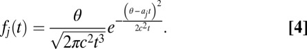Fig. 1.

(A) Task. Subjects fixated on the fixation cross, viewed the display image, and then looked at the gray region coincident with their chosen item and pressed the spacebar. (B) Calculation of saliency and value ranks. Saliency map for display image was obtained with EyeQuant Attention Analytics software, which includes standard channels such as color, intensity, and orientation, as well as shapes. To obtain ranks, pixel values are summed in the region corresponding to each object and ranked (4 = highest, 1 = lowest). Value ranks are obtained by looking up the liking rating for each item shown (4 = highest, 1 = lowest). (C) Calculation of . (Top) , the probability that each item’s DDM unit (Inset) reaches a threshold for an arbitrary fixation in the sequence. Drifts shown in Inset are calculated from saliency and value ranks shown in B according the equation . Solid blue line indicates of the example unit of interest. (Middle) with the same color code as in Top. There is no blue because this is the item of interest. is shown as a thick black line. 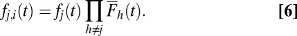(Bottom) (from Eq. 6), i.e., the probability of transitioning from the currently fixated item, i, to item j. The currently fixated item could be any item except the blue item. Shaded region corresponds to Eq. 7 result for the blue unit. There is only a small probability that the blue unit will cross the threshold first, with this event occurring near 190 ms.

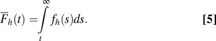
To determine the probability that each accumulator j will reach the threshold first as a function of time, we multiply the probability density function for the jth accumulator, , by the survival function, , for all other accumulators as shown in Eq. 6. Fig. 1C shows this operation for an example case of four alternatives:

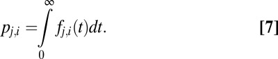
By integrating Eq. 6 over all positive time, we obtain the probability that the acculumator is the first to cross the threshold. In our formulation, this is equivalent to the probability that the gaze transitions from the current location i to location j, namely, the transition probability :

Accounting for cortical processing and movement planning/execution delays.

Eq. 6 describes the probability of making the decision as a function of time. Importantly, because we are measuring the decision in terms of eye movements, the dwell time that we measure includes not only the time required to make the decision, but also the time to extract the object features and the time required to plan and execute an eye movement. As discussed in the introduction, there is a large body of evidence suggesting that the decision process about where to look next occurs in the FEF (24, 26–36).

On the basis of data from neurophysiological measurements in awake monkeys, we can assume that the delay between the retina and the FEF is normally distributed at 75 ± 10 ms (44). Similarly, in awake monkeys, studies have shown that the delay between FEF threshold crossings and eye movements is normally distributed at 30 ± 10 ms (45). To include these delays in our model, we simply convolve the result of Eq. 6 with a normal distribution centered at 75 ms and a normal distribution centered at 30 ms, both with a SD of 10 ms. Because these distributions are probability density distributions and thus integrate to one, the magnitude of the distribution should not change as a result of this convolution:

Importantly, another candidate region for the decision process about where to look next is the lateral interparietal cortex (LIP) (cf. ref. 10). However, the latency to LIP is normally distributed at 90 ± 10 ms (44) and so the discrepancy should be only 15 ms (or 7% of a typical fixation duration). Changing the latency to cortex by 15 ms does not change the results of this study in any way.

Use the Markov property to determine .

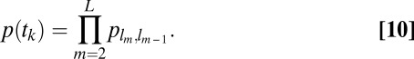
Eq. 7 is the probability of transitioning from location i to location j. To determine the probability of visiting a certain sequence of L locations , i.e., following trajectory , we assume the Markov property. In this context, this means that the probability of fixating on an item does not depend on any past history of fixations, including whether or not one is currently fixated on a certain item. We can therefore multiply the probabilities of making each transition together as in Eq. 10. We show that the Markov property is a good assumption for our data in Results:

Importantly, because subjects make relatively few transitions during each trial, we assume that each transition is similar and thus we treat the initial fixations (i.e., the transition away from the fixation cross-location made by the first saccade) the same as later fixations. Furthermore, as we show in Results, subjects often make refixations onto the same items and so we have allowed refixations in the model. This means that is the probability of making a transition from the current item onto the current item as a function of time or of remaining at the same location. In practice, subjects typically fixate on a different part of the packaging when refixating on the same item. Future versions of the model could easily take this into account by increasing the granularity over which saliency is calculated.

The Conditional Choice Model of .

Using the equations above, we can calculate the probability of every possible gaze trajectory, including its associated temporal structure. To calculate we also need to determine the probability of choosing each item in a display based on this gaze trajectory, . To do this, we use a modified version of the model proposed in ref. 8. The basic idea behind this model is that the longer you spend looking at an item that you like, the more likely you are to choose that item. Mathematically, this is modeled as a DDM, where the drift is proportional to the value of the item and scaled by whether or not you are looking at it. In contrast to the gaze model, the conditional choice model operates on the difference between the accumulators rather than on the absolute value of the accumulators. The difference between accumulators is defined as a “max-vs.-next” operation where the absolute value of the next-highest accumulator is subtracted from the absolute value of a particular accumulator. More concretely, the model follows the following equations.

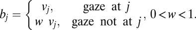
The drift associated with each item is defined as the value of the item j multiplied by a scale factor (w) that is less than 1 when the item is not being looked at:

A drift–diffusion process then describes how each item accumulates “information” subject to the same equation we used for the gaze model, Eq. 2,

where and (6, 8, 9). Importantly, the models described in the Krajbich and Rangel papers (6, 8, 9) all assume that the noise (or spread of the drift) at each time step is constant. This assumption causes their model to differ from the standard drift–diffusion model, where the noise is a function of time (46). Ultimately, a model with a constant noise term will predict a Gaussian and much narrower reaction time distribution, whereas a model with a time-dependent noise term will predict an inverse Gaussian, a much broader and more skewed reaction time distribution. Because reaction times are commonly known to have a right-skewed distribution (Fig. 2), we use the standard drift–diffusion model with a time-dependent noise term .

Fig. 2.

Probability of choosing an item as a function of the time spent looking at it. (A) Individual fixation durations. (Upper) Histogram of fixation durations including all subjects and trials. Shaded line shows fitted inverse Gaussian probability density function. Last bar on right includes all fixations longer than 600 ms. (Lower) Mean ± SEM probability that the item fixated on for a specific duration was ultimately chosen. We use the mean here because probabilities were not significantly different from normal [, Kolmogorov–Smirnov test; 30-ms bins (both Upper and Lower)]. Increase in variance toward 600 ms is due to the low number of samples in this region (Upper). (B) Total dwell time. (Upper) Histogram of total dwell times across all subjects and trials. This distribution had a very long tail (out to 2 s) and the last bar on the right includes all dwell times greater than or equal to 1,000 ms. (Lower) Mean ± SEM probability that the item fixated on for a specific dwell time was ultimately chosen [50-ms bins (both Upper and Lower)]. Chance is 1/4.

Notably, because this is a standard DDM process, the value of at each point in time can be described by the Gaussian in Eq. 12 as shown in Fig. S1:

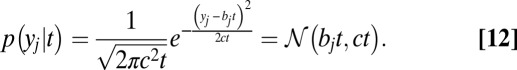Because this is a max-vs.-next process, the random variable of interest is actually the accumulation for each item minus the maximum of the rest of the accumulators at every point in time as shown below. Because these are all Gaussians, the difference is easily computed without need of convolution:

Accordingly, the value of will be increasing only when the accumulator for item j has accumulated more than any other process (Fig. S2). Then the decision problem becomes finding the probability that each is the first to reach a threshold of +1.

Calculating the probability of choosing each item.

To calculate the probability of choosing each item, we consider each possible fixation sequence separately. Using the observed range of fixations to set the range, we considered fixation sequences involving two to six fixations, resulting in 5,456 possible trajectories. For each fixation sequence, we calculate the probability of each relative decision process (from Eq. 13) crossing the threshold of +1. We compute this by integrating the temporal probability distribution described by Eq. 13, evaluated at +1 across all t. This results in the probability that an item n is chosen given a particular trajectory , or . After calculating this for every , by Eq. 1, we compute the total probability of choosing item n by multiplying by the .

Results

Nineteen California Institute of Technology (Caltech) undergraduate students completed an experiment where they were asked to view a 2 × 2 grid of snack food items for 2 s and indicate which item they would like to eat most at the end of the experiment. At the end of the experiment a random trial was chosen and subjects were asked to eat the item they chose on that trial. During the decision process, subjects’ eye movements were measured and used to record their choices. On the basis of subjective preference ratings and quantitative measurement of visual salience, each item could be described in terms of its rank salience and value to the subject. The measured eye movements and rank salience and values form the basis for validating and testing the computational model described above.

Basis of the Model.

Fixation durations predict choices.

The standard drift–diffusion model described above predicts that the fixation durations will follow an inverse Gaussian distribution. Consistent with previous studies (47), we found that the distribution of all fixation durations followed a right-skewed distribution with a median of 214 ms and a median average deviation (MAD) of ±82 ms (Fig. 2A). We use the median to describe this distribution because it is nonnormal. On a per subject basis, this distribution was not significantly different from an inverse Gaussian distribution for all subjects, after removing anticipatory saccades that resulted in fixation durations less than 80 ms (, Kolmogorov–Smirnov test). This demonstrates that the standard DDM is a good choice to model these data.

During the 2-s viewing time subjects made a median of 5 ± 1.2 fixations, ranging between 2 and 10 fixations. There were differences between subjects, with individual subjects ranging from 3 ± 1.1 fixations up to 7 ± 1.3 fixations per trial (median ± MAD). Because the display contained only four different items, subjects often refixated on items that had already been fixated on in the trial. Fig. 2B shows the distribution of the total fixation time on each item (the sum of all fixation durations on the item), which also follows a right-skewed distribution with a median of 390 ± 215 ms.

Using this total fixation duration, we confirmed previous findings (6, 8) that the probability of choosing a particular item increases the longer an item is fixated on (Fig. 2B). The increase is approximately linear, beginning with a zero chance of choosing an item and crossing the chance level between 300 ms and 400 ms. These data are consistent with the predictions of many choice process models, including the aDDM (6–8).

Testing the Markov assumption.

To test whether the Markov property holds, we calculated the probability of fixating on item given that the previous fixation was on location and compared it to the probability of fixating on item given that the previous two fixations had been on items and . For the Markov property to hold, these probabilities should be equal. Indeed, we found no statistical difference between the two distributions and either on an individual subject basis (, -test) or with all subjects pooled (, -test). Thus, the Markov property holds in this dataset and is a reasonable assumption.

Validation of the Gaze Model.

Parameter fits.

The parameter fits were performed as discussed in Materials and Methods. Table 1 shows the fitted values and the fit statistics (, , and ) averaged across all 19 subjects and all seed points. Briefly, is the Pearson -statistic between observed and predicted transition times, is the Akaike information criterion, and is the area under the receiver–operator characteristic (ROC) curve. The _n before each statistic indicates that they were normalized by the number of valid saliency–value combinations for each subject see Materials and Methods for details. Models that have an closer to 1 and smaller and statistics provide a better fit to the data.

Table 1.

Gaze model parameter fits

Parameter or Metric	Model
	s only	v only	s + v	s × v
θ	672 ± 19	630 ± 17	623 ± 12	661 ± 16
c	27 ± 2.4	28 ± 2.0	43 ± 1.4	51 ± 1.5
	3.30 ± 0.15	0	0.42 ± 0.08	1.95 ± 0.16
	0	3.21 ± 0.15	1.45 ± 0.10	2.89 ± 0.17
P of	0.33 ± 0.22	0.61 ± 0.14	0. 77 ± 0.24	0.87 ± 0.21
	141 ± 21	129 ± 21	122 ± 17	116 ± 14
	560 ± 65	483 ± 55	258 ± 23	198 ± 6
	0.63 ± 0.06	0.70 ± 0.06	0.89 ± 0.04	0.93 ± 0.02

Values reported are the mean across subjects ± the SEM.

Table 1 shows four main results. First, the model containing only value information outperforms the model containing only saliency information. Second, the models containing both saliency information and value information provide a better fit to the data than do the models containing only one or the other, even when evaluated with the , which accounts for the increase from three to four parameters. Third, the multiplicative model outperforms the additive model. And, finally, for the combined saliency and value models, saliency has roughly one-third to two-thirds the influence of value.

However, the and fit statistics vary approximately based on which subject was left out of our leave-one-out analysis, making it difficult to establish the difference in fit statistics between the models. Thus, we also looked at the fit statistics for each subject that was left out. Fig. 3 shows the percentage of difference in the between the multiplicative model and the three other models. A positive percentage difference indicates that the multiplicative model had a smaller than the indicated model (and vice versa), and thus fitted the data better (per degree of freedom).

Fig. 3.

Fit comparison between subjects left out. (Top) Percentage of difference between the multiplicative model and the three other models. Ratio of to for the additive model (Middle) and the multiplicative model (Bottom) is shown. Horizontal lines indicate the ratio reported in Table 1. Values plotted are mean ± SEM across subjects and parameter fitting seeds (Materials and Methods).

Fig. 3 shows that for 9 of the 19 subjects, all of the trends from Table 1 remain valid. If we look at each trend on the basis of which subject was left out, we find the following. First, in 14 of the 19 subjects (74%), the value-only model outperforms the saliency-only model. Second, the combined models outperform the saliency-only and value-only models in 15 subjects (79%). And, finally, for 15 subjects (79%), the multiplicative model outperforms all of the other models. Fig. 3 also shows that the ratio of to was robust across subjects, maintaining a ratio near for 11 of the 19 subjects (58%) for the additive model and a ratio near for 16 of the 19 subjects (84%) for the multiplicative model (all verified at , Wilcoxon’s signed-rank test).

Saliency and value are both correlated with the fixation duration.

In addition to predicting the overall fixation sequence with high accuracy (Table 1), the gaze model also predicts how the fixation durations change with increasing value and saliency. From the model equations, it is clear that transitions to highly liked and highly salient items will occur quickly because they will have large drift terms. However, once centered at a highly liked and highly salient location, transitions away from this location will take longer because the magnitude of the drift will be lower. Thus, the model predicts that fixations on highly liked and highly salient items will last longer than fixations on other items. Further, because is 1.5–3 times greater than , the model also predicts that the fixation durations will increase more rapidly as a function of value than as a function of saliency.

Fig. 4A shows the actual fixation durations as a function of value with the modeled fixation durations superimposed. As expected, the model containing only saliency information does not show any difference in the fixation durations as a function of value (P > 0.05, Kruskal–Wallis test). Models containing value information (v only, , and ), however, show an increase in the fixation durations for items with value rankings of 3 or 4 (P < 0.001, Kruskal–Wallis test). Moreover, the multiplicative model fitted the data best, with a P value of 0.71, followed by the additive model (P = 0.67), the value-only model (P = 0.57), and the salience model (P = 0.04, P values of the –goodness-of-fit test).

Fig. 4.

Modeled vs. actual gaze. (A) Fixation durations as a function of value. –goodness-of-fit test: v only, ; s only, ; , ; and , . (B) Fixation durations as a function of saliency. Gray bars indicate actual fixation durations. Model results are shown as colored lines (mean ± SEM) and offset on the x axis to facilitate comparison. Error bars for modeling results were computed across all 576 possible combinations and parameter values. –goodness-of-fit test: v only, ; s only, ; , ; and , . (C) Two actual subject trajectories (white and gray). Number “1” indicates the first fixation location after subjects looked away from the fixation cross. (D) Two computer-simulated gaze trajectories. Locations were offset to allow easier viewing. Circles enclose the fixation locations and the diameter of the circle is proportional to the fixation duration.

Similarly, Fig. 4B shows that the value-only model does not account for the increase in fixation duration as a function of saliency rank (P > 0.05, Kruskal–Wallis test), whereas the combined models follow this increase (P < 0.01, Kruskal–Wallis test). The additive model fitted the data best, with a P value of 0.91, followed by the value-only model (P = 0.85), the salience-only model (P = 0.60), and the multiplicative model (P = 0.53, P values of the –goodness-of-fit test). Interestingly, the multiplicative model and the saliency-only model overpredict the influence of saliency, showing a steeper slope than in the data. The results from Fig. 4 A and B are also consistent when broken down by all combinations of saliency and value, as shown in Figs. S3 and S4. In summary, the multiplicative model fits the data better when grouped by value, but the additive model fits better when grouped by saliency. Thus, we can see that both saliency information and value information are required to predict the fixation durations, although we cannot definitively distinguish between an additive and a multiplicative combination.

Finally, to illustrate the model fits, we also simulated two scan paths from one subject, using the multiplicative model for a randomly chosen image. Fig. 4 C and D shows the actual scan paths and the simulated scan paths for each image. In addition to the quantitative fits above, there is a clear qualitative match between the two.

From the fit statistics and comparison of predicted and actual fixation durations we can see that the multiplicative model tends to perform better than the additive model, although there are exceptions. In Table 1, the metric is lower for the multiplicative model, but the other two fit statistics ( and ) show that the models may have similar accuracy. Thus, on the basis of predicting fixations alone, it would be difficult to claim that one outperformed the other. However, it is possible that one of these models will provide a better account of choices. We investigate this next.

Modeling Choices.

The conditional choice model presented in Materials and Methods is very similar to previously published models showing that by using the actual fixation patterns measured from subjects, a max-vs.-next accumulation model can accurately predict choices (6, 8, 9). This model has been extensively studied in the literature and here we sought to merely demonstrate that our model of fixation patterns can be used as input to this conditional choice model to achieve similar accuracy.

Using the parameters for the gaze model and the parameters reported in ref. 8, we calculated the probability of choosing each item, , as a function of the item’s value and saliency for all 576 possible combinations of value and saliency. Fig. 5 shows the actual probability of choosing an item on the basis of its saliency and value rank as well as the simulated probabilities. Similar to the results for fixation durations, we found that the saliency-only model was uninformative about choice probabilities relative to values and vice versa (P > 0.05, Kruskal–Wallis test). Furthermore, we found that the multiplicative model tended to overemphasize saliency information compared with value information. This is consistent with the fitted values of and for the gaze model, which show that the additive model weights saliency and value in a 1-to-3 ratio and the multiplicative model weights saliency and value in a 2-to-3 ratio.

Fig. 5.

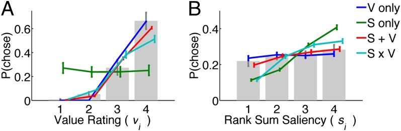
(A and B) Choice probabilities as a function of (A) value and (B) saliency rank. Gray bars and error bars indicate for our data. Model results are shown as colored lines (mean ± SEM) and are offset on the x axis to facilitate comparison. Error bars for modeling results were computed across all 576 possible combinations and parameter values. (A) –goodness-of-fit test: v only, ; s only, ; , ; and , . (B) –goodness-of-fit test: v only, ; s only, ; , ; and , .

Thus, given that the additive and multiplicative models have similar accuracy for predicting gaze, we conclude that the additive model is a better predictor of choices from gaze.

Discussion

We have shown that two independent stochastic accumulator models, one that models the gaze trajectory and one that models the valuation process, can account not only for the pattern of fixations across a display but also for the subsequent choices. Furthermore, we have demonstrated that bottom–up visual saliency influences choices and that it affects the decision process by biasing the location and duration of fixations, but not the valuation process directly. We found that visual fixations are driven by a combination of saliency and value information, likely in a 1-to-3 additive combination or 2-to-3 multiplicative combination. This model brings together modeling approaches from visual neuroscience, decision making, and neuroeconomics to provide a unique perspective on how visually based appetitive decisions are made and influenced by the properties of visual displays.

The Relative Effect of Saliency and Value.

We found that saliency , or bottom–up information, has less of a contribution than value , or top–down information, with a ratio of ∼1-to-3 or 2-to-3 (saliency to value). At least one previous study also investigated the relative effects of saliency and value in a similar task, and, contrary to our findings, reported a ratio of 2:1 (saliency to value) (48). There are two likely reasons for this discrepancy. First, bottom–up saliency was computed differently here. Although van der Lans et al. (48) included three important perceptual features (color, luminance, and edges), these were measured only on a per-pixel basis after smoothing at a single spatial scale. Such an algorithm massively underestimates the effects of neighboring regions on the current region. Our saliency map was generated by measuring many perceptual features (color, luminance, edges, shapes, orientations, etc.) at many different spatial scales (i.e., from single pixels up to groups of pixels) and combining these measurements into a comprehensive saliency map. Second, although top–down information was defined here as an endogenous personal preference, van der Lans et al. (48) used an exogenous definition of top–down information by instructing subjects to look for a specific item before each trial. This type of top–down motivation may correspond well to certain types of tasks (for example, when shopping from someone else’s shopping list). However, our results here indicate that when using personal preferences as a purchasing guide, the effect of top–down information may be much stronger.

One other study has also looked at the effect of saliency and value in economic decision making and, consistent with our results here, concluded that both saliency information and value information are required to explain these choices (49). Importantly, although the Navalpakkam et al. (49) study did not determine the ratio between saliency information and value information or analyze sequences of multiple fixations, it did propose an alternative model of how saliency and value are combined based on Bayesian inference. Their model proposed that expected reward was determined through a multiplicative combination of value (assigned before each trial) and a Bayesian estimate of low-level features such as orientation. Subjects then simply chose the location with the highest expected reward. One very important difference between the model presented here and the Navalpakkam model is that whereas we have assumed visual saliency implicitly affects the final choice process only through biasing fixations, Navalpakkam et al. assumed that visual saliency was explicitly combined with value to calculate the expected reward. We discuss this distinction further below. Although their model fitted their data well, we believe there are several advantages of the DDM-based model proposed here over a Bayesian model. First, the Bayesian approach requires an estimate of stimulus reliability (cf. ref. 50), which is often not available in naturalistic decision making when behavior is not overtrained. Second, Bayesian models do not account for the required decision-making time and thus are ill-suited for modeling the gaze process’s temporal aspect. Finally, a growing body of evidence suggests the firing properties of neurons that likely drive decisions in the LIP and the FEF are well described by stochastic accumulator models (cf. refs. 10 and 24). Although we cannot rule out that a Bayesian model would also model these data well, we believe that stochastic accumulator models provide a more comprehensive explanation of choices that includes time and a neurally plausible implementation.

Importantly, we considered each fixation as independent and grouped all fixations before fitting the model. This approach was necessary here because subjects made relatively few fixations per trial. However, numerous studies have shown that initial fixations may differ from later fixations during visual search tasks (8, 51, 52) and free viewing (53). One difference between this task and other similar tasks is that we used a grayscale mask to enforce a specific viewing time (2 s). A consequence of this manipulation was that the final saccades before choice were often between visually meaningless gray boxes. Thus, we eliminated the final fixations from our analysis because they are likely to be guided by memory and value and not by salient visual information. As mentioned, this study was part of a larger data collection effort and we hope to investigate these saccades in future work.

One intriguing hypothesis for future work comes from studies showing that early fixations are driven toward higher-saliency locations whereas later fixations are driven to more top–down relevant locations (53, 54). Here, value is top–down, so one might expect that the influence of value and saliency would change later in the trial. Namely, one might expect that saliency contributes most to the first fixation and falls off later in the trial, whereas value contribution is lowest early but increases throughout the trial. Unfortunately because subjects made relatively few fixations in this study, our dataset did not provide enough statistical power to test this hypothesis. Future experiments with larger displays to encourage more eye movements could be conducted to test this hypothesis.

The DDM vs. Other Accumulator Models.

Here we have made extensive use of the drift–diffusion model to predict not only fixations but also the valuation process. Although the DDM is a very popular stochastic accumulator model, it is only one of many, including the leaky competing accumulator (5), race (4), the linear approach to threshold with ergodic rate (LATER) (55), the Ornstein–Uhlenbeck model (11), the sequential probability ratio test (SPRT) (56), and indeed, conceptually, even integrate-and-fire neural models (cf. ref. 57). Furthermore, this model does not include additional features that have proved useful elsewhere, such as inhibition (58) or gating (24).

Moreover, whereas the gaze model uses the classical threshold crossing to trigger a decision, the choice model was applied in a fixed-duration paradigm where the subject is asked to make a decision at a specific time. In this task, the decisions are relatively easy to make and may occur before the 2-s viewing period is complete. Practically, this experimental paradigm was chosen to encourage eye movements and to ensure that a sufficient number of eye movements were made in each trial to allow our gaze modeling effort. Providing a very large display with many items would have been an equally effective experimental design, but would have made the computational modeling intractably slow due to the increased number of combinatoric trajectories. However, the fixed-duration experimental design is still consistent with the DDM framework, assuming that the decision, once made, can be held in memory until the end of the trial.

Importantly, the DDM has a distinct advantage over other models in that the time of first passage has been solved for in closed form, significantly simplifying computations (42). Moreover, as shown by Bogacz et al., many of these other models reduce to the DDM under certain parameter assumptions (46). Thus, although accuracy may improve through use of other models and/or features, the model presented here is faster to compute and retains the same basic response features. This makes this model useful for marketers who seek to understand how to design product packaging to gain the most attentional advantage for their products.

The Markov Assumption and Inhibition of Return.

We assume that each fixation is independent of past fixations, namely, the Markov property. However, many studies report that subjects are less likely to look at locations already visited [inhibition of return (IOR)] (59, 60), thus violating the Markov property. Notably, there is some controversy over the IOR effect strength during search and for different measures of IOR (latency, probability of returning to the same location or region, etc.) (60). Although we did not find that subjects were more or less likely to look at items already viewed, it is possible that other measures of IOR would reveal this phenomenon. However, given the 2 × 2 granularity of our search array and that subjects had ample time to search, it is unlikely that a strong effect will emerge. As display sizes and number of options increase, it is possible that IOR will become significant. In this case, the order of the Markov process could be increased to account for some past history of viewing.

A Combined Model of Perceptual and Economic Decision Making.

We have investigated a unique two-part model that links a perceptual decision process with a value-based (economic) decision process. Although each process has been previously modeled with stochastic accumulators, this study combines models of both processes in a single model. To create this integrated model we have made several assumptions.

First, we assume both processes are governed by the same formalisms and can be modeled as stochastic accumulation processes. Although there is some controversy about whether economic and perceptual decisions have similar neurobiological substrates (cf. ref. 61), both have been successfully, and separately, modeled by stochastic accumulator models (10, 40, 62, 63).

Second, we assume that the perceptual decision process integrates absolute evidence and the economic decision process integrates relative evidence on the basis of a max-vs.-next operation. We assumed this on the basis of prevailing trends in both literatures (2). However, because this is an open question in each field separately, it is clearly an open question here as well. We can say that our data support these prevailing trends.

Third, we assume that these processes run in parallel and that the perceptual process is the limiting factor for the economic process. It is widely accepted that during fixation at least two things need to occur: (i) high-quality sensory information needs to be extracted from the (para)foveal region of the eye and (ii) plans need to be made about where to move the eyes next. Given that the visual system is divided into the ventral (“what”) and the dorsal (“where”) pathways, it would seem reasonable that these two tasks are completed in parallel because they are likely to involve different neural substrates (cf. ref. 64). What is currently unclear is which one of these two processes should be the limiting factor. In other words, does the information extraction phase end when the location of future fixation has been determined? Or, conversely, does the eye move when the information extraction phase is complete? In our model we have assumed the former because in this task there is no time pressure and therefore no pressure to gather as much information as possible in a single fixation. It is certainly possible that under different conditions this assumption may need to be reversed.

Fourth, although these processes are distinct, they have access to the same value signals. There is an abundance of evidence to support the claim that the perceptual process could be implemented in visually responsive neurons of the FEF, the LIP, and/or the SC (24, 28, 30, 65–67). Similarly, many recent studies have indicated that the economic decision process takes place in various regions of the frontal and parietal cortices (68–71), including the orbitofrontal cortex (OFC) (72–74), the ventro-medial prefrontal cortex (vmPFC) (75, 76), and the amygdala (77). Connections between putative perceptual decision-making areas (FEF, LIP, and/or SC) and putative economic decision-making areas (OFC, vmPFC, and/or amygdala) abound, creating the possibility that value information is shared directly between these processes. Moreover, many of these areas receive input from common regions, creating the possibility of a common source for value signals in both processes. Thus, we consider this assumption reasonable.

Finally, we assume that the only link between these processes is that the perceptual decision process limits the durations for which the economic decision process is amplified, implying that the perceptual decision process is independent of the economic decision process, but not vice versa. However, it is possible that these processes are more intricately linked (via the anatomical connections discussed above) and that these processes could interact on a more subtle level through modulation between these regions. Such modulation could happen at timescales much shorter than the time required to move the eyes and so may be especially apparent in quick decisions. For the timescale of decisions modeled, however, our results show that we need not assume such an interaction to effectively model both the fixation process and choices.

Model Predictions and Future Directions.

Each of our assumptions can also be seen as a hypothesis to be tested empirically. Although testing each of these assumptions was outside the scope of this paper, future work should investigate whether these assumptions hold as display sizes or search difficulty are increased, for example by including items with the same value.

Despite these assumptions, however, our model is able to predict fixation patterns with accuracy similar to that of other models as measured by (here, 116–141; the best from ref. 24, 106–157), and as measured by (here, 0.89–0.93; ref. 78, 0.83; ref. 79, 0.88; ref. 80, 0.89; ref. 22, 0.90; and ref. 23, 0.95). Moreover, our model can predict choices with better accuracy than previous models that do not model fixation patterns, measured by the P value of the –goodness-of-fit test (here, 0.75–0.90; ref. 8, 0.64).

As presented, this model represents a unique integrated model of perceptual and economic decision making, which has applications not only for understanding the neural basis of decision making, but also to fields such as marketing that have a vested interest in the factors affecting decisions. This model provides a viable alternative to collecting eye-tracking data. Our model uses only the display itself and a measure of subjective value to predict the fixation patterns and durations and subsequently choices. The saliency can be computed a priori and thus does not require extensive experimentation. In addition, there are many established methods for gathering subjective preferences that use either surveys or data about the current market share of various products. Thus, this model provides a framework in which marketers could examine how certain displays affect choices without the need to collect time- and data-intensive eye-tracking data.

Overall, our model makes three unique contributions. In the realm of economic decision making, we extend the aDDM by incorporating a model of the fixation process. In the realm of perceptual decision making, we extend current stochastic models of saccades beyond the first saccade to account for the entire sequence of fixations and fixation durations during visual search for a liked item. And, in the realm of visual decision making as a whole, we present a unique model that combines perceptual and economic decision making to account for choices using only the stimulus as input.

Materials and Methods

Subjects.

Subjects were 16 male and 3 female Caltech students aged from 18 to 30 (mean 21) y and of mixed racial and ethnic backgrounds. Six subjects were eliminated during prescreening because they had never tasted more than six items in this study. At the beginning of the session subjects were instructed to look at the items displayed in each trial and choose the item they most wanted to eat at the end of the experiment (see Trials for details). Subjects were also told that at the end of the experiment, one random trial would be chosen and they would need to eat the item they chose on that trial. This instruction was to motivate subjects to make realistic choices on each trial. Subjects completed five practice trials before the start of the session. These practice trials used stimuli that were not used for data collection.

Measuring “Value”.

At the beginning of the session, subjects viewed individual photographs of each item that they would be choosing among during the session. There were 41 snack food items in total. After the initial viewing, subjects rated how much they would like to eat each item on a Likert scale from “1” (“would not like to eat at all”) to “5” (“would like to eat very much”). If subjects had never tasted the item, they marked it as a “3” and these items were excluded from the possible stimuli. Thus, valid liking ratings were 1, 2, 4, and 5; however, to avoid confusion, these ratings were recoded to 1, 2, 3, and 4 for the analysis and modeling. If subjects had never tasted more than 6 items of the 41 items (14.6%), they were eliminated from this study. The subject’s liking ratings were considered to be the subject’s “value” of each item. Previous research has demonstrated that dollar willingness-to-pay for similar foods is highly correlated with liking ratings (74, 81, 82), as well as charities (75), and thus liking ratings are considered a reasonable measure of intrinsic value.

Measuring Salience.

The stimuli originated from 100 photographs of 28 snack food items (e.g., chips and candy) arranged on a shelf in four rows and seven columns in a random order. From each photograph, we created 18 different stimuli by cropping out groups of 4 items in a 2 × 2 arrangement and applying a Gaussian smoothing function to the cropped edges. An example stimulus is shown in Fig. 1A. This procedure produced 1,800 possible stimuli. For each stimulus, the saliency map was computed across the entire image, using an extended version of the Itti–Koch algorithm (78), including proprietary channels developed by EyeQuant Attention Analytics (www.eyequant.com) (Fig. 1B). Unlike standard saliency algorithms (e.g., those available at ilab.usc.edu/toolkit and saliencytoolbox.net), EyeQuant software is optimized using machine learning techniques to deal with Web-page images, which contain large regions of a solid background color similar to the images used in our experiments. We then computed the “rank-sum saliency” from this map by taking the sum of all pixels in the region corresponding to each item and ranking the sums in ascending order (lowest rank sum saliency = 1, highest rank sum saliency = 4).

Importantly, the saliency of a single item varied from display to display, depending on what items were surrounding it. For example, when a relatively bright item, such as Lays Classic potato chips, is surrounded by items of similar brightness (e.g., other items with predominantly yellow packaging), the saliency rank of the Lays Classic potato chips will likely be lower than when that item is surrounded by relatively dark items such as chocolate. Thus, the saliency rank of each item was computed independently for all possible displays and each item had a range of saliency ranks (one per display).

Because we did not manipulate salience, we carefully investigated our stimulus images to ensure that the range of saliencies was sufficiently large to measure a meaningful effect and that the salience ranks indicated legitimate changes in salience and not just variations on the order of one or two pixels.

We determined the total salience for each display and then calculated the salience of each item as the percentage of this total possible salience. If the salience range were small, then we would expect the range and SD of percentage saliencies to be small as well. However, we found that the range of percentage saliencies was from 13.5% to 40.6% (27.1% average) and the SD was ±5.1%, indicating that item salience existed over a meaningful range.

Moreover, in a single display, the difference in percentage salience between pairs of items ranged from −14.8% to 13.7% (28.6% average range) with a SD of ±4%, demonstrating that the item salience in a single display typically represented substantial differences in salience. A one-way ANOVA verified that there was a significant difference between the percentage salience associated with different ranks (P = 1.17 × 10⁻⁶⁷, F = 145.57, one-way ANOVA). Further analysis revealed that the mean difference was 2.3 ± 1.1% (±SD) of the total image salience. Thus, images provided a large range of salience values providing a meaningful measure and the salience ranks indicate a legitimate salience change between items.

Stimuli.

From the measures of value and salience described above, for each four-item stimulus we have a measure of the values of each item in the image (1, 2, 3, or 4 for each item) and the saliency of the items in the image (1, 2, 3, or 4). Stimuli were excluded from the final stimulus set if there were items with the same value in the stimulus or items that the subject had never tasted. This exclusion produced 24 possible saliency permutations and 24 possible value permutations, for a total of 576 possible saliency–value permutations in the stimuli.

However, because the photographs from which the stimuli came did not span all possible permutations of the items (we created 100 permutations of the possible), there was a limit to the number of the 576 saliency–value combinations that we could produce for each subject. The number of permutations for each individual subject ranged from 12 to 110 with a median of 47.

Within each subject we also ensured that there was no correlation between the saliency and the value of any option (minimum r² = 0.21 with a P value = 0.542, F-test). The value was constant across all trials within a subject, but the saliency varied on the basis of the particular combination of items in the display as explained above.

Familiarity.

In our experiment, salience was defined to account only for bottom–up factors. A subject’s history with an item was not considered a bottom–up feature because this is not exogenous to the item itself, but rather endogenous to the subject. We did consider, however, that a subject’s familiarity with an item might be a separate top–down factor that could bias the subject’s gaze and choices. Because we are working with human subjects that will inevitably have different experiences with these items, a perfect control for familiarity was not possible. However, we endeavored to control for familiarity in the following three ways.

First, we did not use items unfamiliar to subjects in the displays shown to that subject. Second, we recruited only subjects that reported that they really liked junk food to increase the chances of subjects being equally familiar with all items. Third, in a subset of subjects we collected familiarity ratings as well as value ratings. These were collected in the same way as value ratings; namely, subjects had to rank each item individually from 1 (“Not at all familiar: I have never seen this item before”) to 5 [“Extremely familiar: I eat this item regularly (at least once a month)”].

We found that a subject’s familiarity with an item (range from 2 to 5 because items of familiarity 1 were not used) was not correlated with either the subject’s value for that item (mean across subjects = 0.09) or the subject’s probability of choosing that item (mean across subjects = 0.11). Under conditions of time pressure or very large displays, these relations may change. However, for the purposes of this experiment, we do not consider familiarity to play a large role in subjects’ choice behavior.

Trials.

Each trial consisted of three phases. First, subjects fixated on a gray fixation cross for 500 ms. To minimize the effect of the center bias (83, 84), this fixation cross was randomly displayed at the location of 1 of the 4 items subsequently shown. Further, the grid of 4 items was located randomly at 1 of 18 locations on the screen. Second, the stimulus with 4 items appeared on the screen and subjects were permitted to freely look around the stimulus for 2 s. Preliminary data revealed that 2 s was ample time for subjects to make this type of choice. In addition, previous research found that participants typically make similar types of decisions in less than 2 s (6, 81, 85) and even that subjects can make accurate choices among 16 food items in less than 3 s (86). During this phase, eye movements were recorded at 1,000 Hz with an EyeLink 1000 (SR Research). After the 2-s exposure time, the stimulus was replaced with the grayscale mask shown in Fig. 1A. Third, subjects looked at the gray region at the location of their chosen item and pressed the spacebar. Choices were measured by computing which gray region contained the subject’s gaze at the time of the spacebar press. This task was a part of a larger data collection effort, not all of which is reported here. Tasks were counterbalanced to avoid any cross-contamination from other tasks.

Each subject performed a number of trials set by the number of possible permutations and the number of stimuli in the set that matched those permutations. For each individual subject the number of trials ranged from 29 to 133 with a median of 95. Importantly, during these trials, all subjects were presented with multiple items in each of the 16 salience–value combinations.

Parameter Fitting.

We fitted the parameters of the gaze model , using a leave-one-subject-out cross-validation. In other words, the model is fitted on the basis of the data of 18 subjects, leaving 1 subject out, and then the fitted parameters are tested with the data from the left-out subject. This is repeated 19 times, each time leaving out a different subject. The optimization was performed using Matlab’s interior-point algorithm (The Mathworks) with constraints to ensure that the threshold θ was greater than the noise c, that k was greater than (where necessary), and that none of the parameters fell below zero. The optimization was performed from 10 different seed points to ensure the robustness of our parameter fits.

The fit was performed by minimizing the Pearson -statistic between the observed transition times and the predicted transition times. All transitions were considered independent, following the assumed Markov property. For each possible transition , the Pearson -statistic was computed by taking the difference of the frequency of observed and predicted transition times falling within bins defined by the 10th, 30th, 50th, 70th, and 90th percentiles after the methods of Van Zandt (87) and Ratcliff and Tuerlinckx (88). Because the predicted transition times followed a continuous probability distribution function (Eq. 8), they were converted to frequencies by multiplying by the total number of observed transitions (n). The statistic was summed across each of the 16 possible transitions and all possible saliency and value combinations according to the following equation:

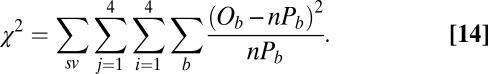We also computed two other metrics to assess our model fits. The first is a version of the area-under-the-ROC curve statistic that is more intuitive than the -statistic. For the ROC analysis, we considered each combination of saliency and value separately. For a given combination, all transitions were calculated from the equations above. Then, for each possible transition , we systematically lowered a threshold from the maximum of the transition time probability curve to zero in 100 steps and calculated the number of subject fixations that were coincident with the part of the probability distribution above the threshold (hits) and the number that were not coincident with this portion (false positives). Fig. S5 illustrates this process. For each transition pair we also counted the total number of transitions (number of positives) and the number of time bins in which no transition occurred (number of negatives).

These four numbers were calculated for each of the 16 possible transitions . The ROC for a given saliency and value combination was then calculated by summing the total number of hits and dividing it by the total number of transitions (positives) to get the true positive rate and plotting this against the false positive rate (calculated as the sum of false positives divided by the total number of negatives). The AUC was then computed from the graph. Fig. S5 shows an example of this procedure. Because of intersubject variability, the model could not be expected to perform better than the AUC obtained by using one subject to predict another. Thus, we normalized the model AUC values by the average ideal AUC obtained by using a single subject’s data to predict the remaining n − 1 subjects’ data, which was 0.90 for this dataset. Normalized values are reported as . The second metric was used to assess whether model fits improved simply due to the addition of more parameters (M is the number of free parameters for each model). The metric chosen was the AIC, which is a penalized maximum-likelihood statistic. Like the statistic, the AIC was computed from the frequency of observed and predicted transition times falling within bins defined by the 10th, 30th, 50th, 70th, and 90th percentiles. Eq. 15 shows how this statistic was computed:

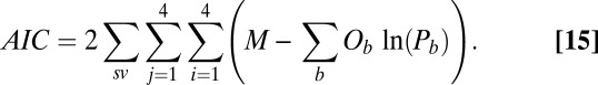To compare the - and AIC statistics across subjects with different numbers of valid saliency and value combinations , we divided each statistic by the number of valid combinations for each subject to get the average value for the statistic per saliency–value combination such that and . Model performance increases as the approaches 1 and as and decrease.

References

- 1.Summerfield C, Tsetsos K. Building bridges between perceptual and economic decision-making: Neural and computational mechanisms. Front Neurosci. 2012;6:70. doi: 10.3389/fnins.2012.00070. [DOI] [PMC free article] [PubMed] [Google Scholar]
- 2.Milosavljevic M, Navalpakkam V, Koch C, Rangel A. Relative visual saliency differences induce sizable bias in consumer choice. J Consum Psychol. 2012;22(1):67–74. [Google Scholar]
- 3.Smith PL, Ratcliff R. Psychology and neurobiology of simple decisions. Trends Neurosci. 2004;27(3):161–168. doi: 10.1016/j.tins.2004.01.006. [DOI] [PubMed] [Google Scholar]
- 4. Vickers D (1979) Decision Processes in Visual Perception (Academic Press, New York), pp 374–396.
- 5.Usher M, McClelland JL. The time course of perceptual choice: The leaky, competing accumulator model. Psychol Rev. 2001;108(3):550–592. doi: 10.1037/0033-295x.108.3.550. [DOI] [PubMed] [Google Scholar]
- 6.Krajbich I, Armel C, Rangel A. Visual fixations and the computation and comparison of value in simple choice. Nat Neurosci. 2010;13(10):1292–1298. doi: 10.1038/nn.2635. [DOI] [PubMed] [Google Scholar]
- 7.Milosavljevic M, Malmaud J, Huth A, Koch C, Rangel A. The drift diffusion model can account for the accuracy and reaction time of value-based choices under high and low time pressure. Judgm Decis Mak. 2010;5(6):437–449. [Google Scholar]
- 8.Krajbich I, Rangel A. Multialternative drift-diffusion model predicts the relationship between visual fixations and choice in value-based decisions. Proc Natl Acad Sci USA. 2011;108(33):13852–13857. doi: 10.1073/pnas.1101328108. [DOI] [PMC free article] [PubMed] [Google Scholar]
- 9.Krajbich I, Lu D, Camerer C, Rangel A. The attentional drift-diffusion model extends to simple purchasing decisions. Front Psychol. 2012;3:193. doi: 10.3389/fpsyg.2012.00193. [DOI] [PMC free article] [PubMed] [Google Scholar]
- 10.Gold JI, Shadlen MN. The neural basis of decision making. Annu Rev Neurosci. 2007;30:535–574. doi: 10.1146/annurev.neuro.29.051605.113038. [DOI] [PubMed] [Google Scholar]
- 11.Busemeyer JR, Townsend JT. Decision field theory: A dynamic-cognitive approach to decision making in an uncertain environment. Psychol Rev. 1993;100(3):432–459. doi: 10.1037/0033-295x.100.3.432. [DOI] [PubMed] [Google Scholar]
- 12.Usher M, McClelland JL. Loss aversion and inhibition in dynamical models of multialternative choice. Psychol Rev. 2004;111(3):757–769. doi: 10.1037/0033-295X.111.3.757. [DOI] [PubMed] [Google Scholar]
- 13.Kustov AA, Robinson DL. Shared neural control of attentional shifts and eye movements. Nature. 1996;384(6604):74–77. doi: 10.1038/384074a0. [DOI] [PubMed] [Google Scholar]
- 14.Mohler CW, Wurtz RH. Organization of monkey superior colliculus: Intermediate layer cells discharging before eye movements. J Neurophysiol. 1976;39(4):722–744. doi: 10.1152/jn.1976.39.4.722. [DOI] [PubMed] [Google Scholar]
- 15.Walther D, Koch C. Modeling attention to salient proto-objects. Neural Netw. 2006;19(9):1395–1407. doi: 10.1016/j.neunet.2006.10.001. [DOI] [PubMed] [Google Scholar]
- 16.Reichle ED, Rayner K, Pollatsek A. The E-Z reader model of eye-movement control in reading: Comparisons to other models. Behav Brain Sci. 2003;26(4):445–476, discussion 477–526. doi: 10.1017/s0140525x03000104. [DOI] [PubMed] [Google Scholar]
- 17. Wolfe JM (2007) Guided Search 4.0: Current Progress with a Model of Visual Search in Integrated Models of Cognitive Systems, ed. Gray WD (Oxford Univ Press, New York), pp 99–119.
- 18.Treisman A, Gormican S. Feature analysis in early vision: Evidence from search asymmetries. Psychol Rev. 1988;95(1):15–48. doi: 10.1037/0033-295x.95.1.15. [DOI] [PubMed] [Google Scholar]
- 19.Navalpakkam V, Itti L. Search goal tunes visual features optimally. Neuron. 2007;53(4):605–617. doi: 10.1016/j.neuron.2007.01.018. [DOI] [PubMed] [Google Scholar]
- 20.Bundesen C, Habekost T, Kyllingsbaek S. A neural theory of visual attention: Bridging cognition and neurophysiology. Psychol Rev. 2005;112(2):291–328. doi: 10.1037/0033-295X.112.2.291. [DOI] [PubMed] [Google Scholar]
- 21.Itti L, Koch C. Computational modelling of visual attention. Nat Rev Neurosci. 2001;2(3):194–203. doi: 10.1038/35058500. [DOI] [PubMed] [Google Scholar]
- 22. Hou X, Zhang L (2008) Dynamic visual attention: Searching for coding length increments. Advances in Neural Information Processing Systems, eds Koller D, Schuurmans D, Bengio Y, Bottou L, Culotta A (MIT Press, Cambridge, MA), pp 651–688.
- 23.Zhao Q, Koch C. Learning a saliency map using fixated locations in natural scenes. J Vis. 2011;11(3):1–15. doi: 10.1167/11.3.9. [DOI] [PubMed] [Google Scholar]
- 24.Purcell BA, Schall JD, Logan GD, Palmeri TJ. From salience to saccades: Multiple-alternative gated stochastic accumulator model of visual search. J Neurosci. 2012;32(10):3433–3446. doi: 10.1523/JNEUROSCI.4622-11.2012. [DOI] [PMC free article] [PubMed] [Google Scholar]
- 25.Schall JD, Purcell BA, Heitz RP, Logan GD, Palmeri TJ. Neural mechanisms of saccade target selection: Gated accumulator model of the visual-motor cascade. Eur J Neurosci. 2011;33(11):1991–2002. doi: 10.1111/j.1460-9568.2011.07715.x. [DOI] [PMC free article] [PubMed] [Google Scholar]
- 26.Schall JD, Hanes DP. Neural basis of saccade target selection in frontal eye field during visual-search. Nature. 1993;366(6454):467–469. doi: 10.1038/366467a0. [DOI] [PubMed] [Google Scholar]
- 27.Gottlieb JP, Kusunoki M, Goldberg ME. The representation of visual salience in monkey parietal cortex. Nature. 1998;391(6666):481–484. doi: 10.1038/35135. [DOI] [PubMed] [Google Scholar]
- 28.Bichot NP, Schall JD. Effects of similarity and history on neural mechanisms of visual selection. Nat Neurosci. 1999;2(6):549–554. doi: 10.1038/9205. [DOI] [PubMed] [Google Scholar]
- 29.Constantinidis C, Steinmetz MA. Posterior parietal cortex automatically encodes the location of salient stimuli. J Neurosci. 2005;25(1):233–238. doi: 10.1523/JNEUROSCI.3379-04.2005. [DOI] [PMC free article] [PubMed] [Google Scholar]
- 30.Ipata AE, Gee AL, Gottlieb J, Bisley JW, Goldberg ME. LIP responses to a popout stimulus are reduced if it is overtly ignored. Nat Neurosci. 2006;9(8):1071–1076. doi: 10.1038/nn1734. [DOI] [PMC free article] [PubMed] [Google Scholar]
- 31.Thomas NWD, Paré M. Temporal processing of saccade targets in parietal cortex area LIP during visual search. J Neurophysiol. 2007;97(1):942–947. doi: 10.1152/jn.00413.2006. [DOI] [PubMed] [Google Scholar]
- 32.Hanes DP, Schall JD. Neural control of voluntary movement initiation. Science. 1996;274(5286):427–430. doi: 10.1126/science.274.5286.427. [DOI] [PubMed] [Google Scholar]
- 33.Hanes DP, Patterson WF, 2nd, Schall JD. Role of frontal eye fields in countermanding saccades: Visual, movement, and fixation activity. J Neurophysiol. 1998;79(2):817–834. doi: 10.1152/jn.1998.79.2.817. [DOI] [PubMed] [Google Scholar]
- 34.Paré M, Hanes DP. Controlled movement processing: Superior colliculus activity associated with countermanded saccades. J Neurosci. 2003;23(16):6480–6489. doi: 10.1523/JNEUROSCI.23-16-06480.2003. [DOI] [PMC free article] [PubMed] [Google Scholar]
- 35.Boucher L, Palmeri TJ, Logan GD, Schall JD. Inhibitory control in mind and brain: An interactive race model of countermanding saccades. Psychol Rev. 2007;114(2):376–397. doi: 10.1037/0033-295X.114.2.376. [DOI] [PubMed] [Google Scholar]
- 36.Ratcliff R, Hasegawa YT, Hasegawa RP, Smith PL, Segraves MA. Dual diffusion model for single-cell recording data from the superior colliculus in a brightness-discrimination task. J Neurophysiol. 2007;97(2):1756–1774. doi: 10.1152/jn.00393.2006. [DOI] [PMC free article] [PubMed] [Google Scholar]
- 37.Shimojo S, Simion C, Shimojo E, Scheier C. Gaze bias both reflects and influences preference. Nat Neurosci. 2003;6(12):1317–1322. doi: 10.1038/nn1150. [DOI] [PubMed] [Google Scholar]
- 38. Summerfield C, Koechlin E (2010) Economic value biases uncertain perceptual choices in the parietal and prefrontal cortices. Front Hum Neurosci 4:208. [DOI] [PMC free article] [PubMed]
- 39.McMillen T, Holmes P. The dynamics of choice among multiple alternatives. J Math Psychol. 2006;50(1):30–57. [Google Scholar]
- 40. Busemeyer JR, Johnson JG (2004) Computational models of decision making. Blackwell Handbook of Judgment and Decision Making, eds Koehler DJ, Harvey N (Blackwell Publishing, Oxford), pp 133–154.
- 41.Bogacz R. Optimal decision-making theories: Linking neurobiology with behaviour. Trends Cogn Sci. 2007;11(3):118–125. doi: 10.1016/j.tics.2006.12.006. [DOI] [PubMed] [Google Scholar]
- 42.Schrödinger E. The theory of drop and rise tests on Brownian motion particles. Phys Z. 1915;16:289–295. [Google Scholar]
- 43.Smoluchowski M. Notes on the calculation of the Brownian motion of molecules in Millikan-honourable test arrangements. Phys Z. 1915;16:318–321. [Google Scholar]
- 44.Schmolesky MT, et al. Signal timing across the macaque visual system. J Neurophysiol. 1998;79(6):3272–3278. doi: 10.1152/jn.1998.79.6.3272. [DOI] [PubMed] [Google Scholar]
- 45. Wurtz RH, Goldberg ME (1972) Activity of superior colliculus in behaving monkey. 3. Cells discharging before eye-movements. J Neurophysiol 35(4):575–586. [DOI] [PubMed]
- 46.Bogacz R, Brown E, Moehlis J, Holmes P, Cohen JD. The physics of optimal decision making: A formal analysis of models of performance in two-alternative forced-choice tasks. Psychol Rev. 2006;113(4):700–765. doi: 10.1037/0033-295X.113.4.700. [DOI] [PubMed] [Google Scholar]
- 47.White CT, Eason RG, Bartlett NR. Latency and duration of eye movements in the horizontal plane. J Opt Soc Am. 1962;52(2):210–213. doi: 10.1364/josa.52.000210. [DOI] [PubMed] [Google Scholar]
- 48.Van Der Lans R, Pieters R, Wedel M. Competitive brand salience. Mark Sci. 2008;27(5):922–931. [Google Scholar]
- 49.Navalpakkam V, Koch C, Rangel A, Perona P. Optimal reward harvesting in complex perceptual environments. Proc Natl Acad Sci USA. 2010;107(11):5232–5237. doi: 10.1073/pnas.0911972107. [DOI] [PMC free article] [PubMed] [Google Scholar]
- 50.Yuille A, Bulthoff HH. Bayesian Decision Theory and Psychophysics in Perception as Bayesian Inference. Cambridge, UK: Cambridge Univ Press; 1996. pp. 123–162. [Google Scholar]
- 51.Markowitz DA, Shewcraft RA, Wong YT, Pesaran B. Competition for visual selection in the oculomotor system. J Neurosci. 2011;31(25):9298–9306. doi: 10.1523/JNEUROSCI.0908-11.2011. [DOI] [PMC free article] [PubMed] [Google Scholar]
- 52.Theeuwes J. Top-down and bottom-up control of visual selection. Acta Psychol. 2010;135(2):77–99. doi: 10.1016/j.actpsy.2010.02.006. [DOI] [PubMed] [Google Scholar]
- 53.Mackay M, Cerf M, Koch C. Evidence for two distinct mechanisms directing gaze in natural scenes. J Vis. 2012;12(4):9. doi: 10.1167/12.4.9. [DOI] [PubMed] [Google Scholar]
- 54.Mannan SK, Kennard C, Husain M. The role of visual salience in directing eye movements in visual object agnosia. Curr Biol. 2009;19(6):R247–R248. doi: 10.1016/j.cub.2009.02.020. [DOI] [PubMed] [Google Scholar]
- 55.Reddi BAJ, Carpenter RHS. The influence of urgency on decision time. Nat Neurosci. 2000;3(8):827–830. doi: 10.1038/77739. [DOI] [PubMed] [Google Scholar]
- 56. Wald A (1947) Foundations of a general theory of sequential decision functions. Econometrica 15(4):279–313.
- 57. Koch C, Idan S (1998) Methods in Neuronal Modeling (MIT Press, Cambridge, MA)
- 58.Ditterich J, Mazurek ME, Shadlen MN. Microstimulation of visual cortex affects the speed of perceptual decisions. Nat Neurosci. 2003;6(8):891–898. doi: 10.1038/nn1094. [DOI] [PubMed] [Google Scholar]
- 59. Posner MI, Cohen Y (1984) Components of visual orienting. Attention and Performance X: Control of Language Processes, 32, eds Bouma H, Bouwhuis DG (Erlbaum, Hilsdale, NJ) pp 531–556.
- 60.Klein RM. Inhibition of return. Trends Cogn Sci. 2000;4(4):138–147. doi: 10.1016/s1364-6613(00)01452-2. [DOI] [PubMed] [Google Scholar]
- 61. Shadlen MN, Kiani R, Hanks TD, Churchland AK (2008) Neurobiology of decision making: An intentional framework. Better Than Conscious?, eds. Engel C, Singer W (MIT Press, Cambridge, MA), pp 71–101.
- 62.Rangel A, Camerer CF, Montague PR. A framework for studying the neurobiology of value-based decision making. Nat Rev Neurosci. 2008;9(7):545–556. doi: 10.1038/nrn2357. [DOI] [PMC free article] [PubMed] [Google Scholar]
- 63.Kable JW, Glimcher PW. The neurobiology of decision: Consensus and controversy. Neuron. 2009;63(6):733–745. doi: 10.1016/j.neuron.2009.09.003. [DOI] [PMC free article] [PubMed] [Google Scholar]
- 64. Ungerleider LG, Mishkin M (1982) Two cortical visual systems. Analysis of Visual Behavior, eds Ingle DJ, Goodale MA, Mansfield RJW (MIT Press, Cambridge, MA), pp 549–586.
- 65.Thompson KG, Bichot NP. A visual salience map in the primate frontal eye field. Prog Brain Res. 2005;147:251–262. doi: 10.1016/S0079-6123(04)47019-8. [DOI] [PubMed] [Google Scholar]
- 66.Fecteau JH, Munoz DP. Salience, relevance, and firing: A priority map for target selection. Trends Cogn Sci. 2006;10(8):382–390. doi: 10.1016/j.tics.2006.06.011. [DOI] [PubMed] [Google Scholar]
- 67.Bisley JW, Goldberg ME. Attention, intention, and priority in the parietal lobe. Annu Rev Neurosci. 2010;33:1–21. doi: 10.1146/annurev-neuro-060909-152823. [DOI] [PMC free article] [PubMed] [Google Scholar]
- 68.Montague PR, Berns GS. Neural economics and the biological substrates of valuation. Neuron. 2002;36(2):265–284. doi: 10.1016/s0896-6273(02)00974-1. [DOI] [PubMed] [Google Scholar]
- 69.Platt ML, Glimcher PW. Response fields of intraparietal neurons quantified with multiple saccadic targets. Exp Brain Res. 1998;121(1):65–75. doi: 10.1007/s002210050438. [DOI] [PubMed] [Google Scholar]
- 70.Musallam S, Corneil BD, Greger B, Scherberger H, Andersen RA. Cognitive control signals for neural prosthetics. Science. 2004;305(5681):258–262. doi: 10.1126/science.1097938. [DOI] [PubMed] [Google Scholar]
- 71.Schultz J, Imamizu H, Kawato M, Frith CD. Activation of the human superior temporal gyrus during observation of goal attribution by intentional objects. J Cogn Neurosci. 2004;16(10):1695–1705. doi: 10.1162/0898929042947874. [DOI] [PubMed] [Google Scholar]
- 72.Padoa-Schioppa C, Assad JA. Neurons in the orbitofrontal cortex encode economic value. Nature. 2006;441(7090):223–226. doi: 10.1038/nature04676. [DOI] [PMC free article] [PubMed] [Google Scholar]
- 73.Deaner RO, Khera AV, Platt ML. Monkeys pay per view: Adaptive valuation of social images by rhesus macaques. Curr Biol. 2005;15(6):543–548. doi: 10.1016/j.cub.2005.01.044. [DOI] [PubMed] [Google Scholar]
- 74.Plassmann H, O’Doherty JP, Rangel A. Orbitofrontal cortex encodes willingness to pay in everyday economic transactions. J Neurosci. 2007;27(37):9984–9988. doi: 10.1523/JNEUROSCI.2131-07.2007. [DOI] [PMC free article] [PubMed] [Google Scholar]
- 75.Hare TA, Camerer CF, Knoepfle DT, Rangel A. Value computations in ventral medial prefrontal cortex during charitable decision making incorporate input from regions involved in social cognition. J Neurosci. 2010;30(2):583–590. doi: 10.1523/JNEUROSCI.4089-09.2010. [DOI] [PMC free article] [PubMed] [Google Scholar]
- 76.Lim SL, O’Doherty JP, Rangel A. The decision value computations in the vmPFC and striatum use a relative value code that is guided by visual attention. J Neurosci. 2011;31(37):13214–13223. doi: 10.1523/JNEUROSCI.1246-11.2011. [DOI] [PMC free article] [PubMed] [Google Scholar]
- 77.Jenison RL, Rangel A, Oya H, Kawasaki H, Howard MA. Value encoding in single neurons in the human amygdala during decision making. J Neurosci. 2011;31(1):331–338. doi: 10.1523/JNEUROSCI.4461-10.2011. [DOI] [PMC free article] [PubMed] [Google Scholar]
- 78. Itti L, Koch C, Niebur E (1998) A model of saliency-based visual attention for rapid scene analysis. IEEE Trans Patt Anal Machine Intell 20(11):1254–1259.
- 79. Gao D, Mahadevan V, Vasconcelos N (2007) The discriminant center-surround hypothesis for bottom-up saliency. Advances in Neural Information Processing Systems 20, eds Platt JC, Koller D, Singer Y, Roweis S (MIT Press, Cambridge, MA), pp 497–504.
- 80.Bruce ND, Tsotsos JK. Saliency, attention, and visual search: An information theoretic approach. J Vis. 2009;9(3):1–24. doi: 10.1167/9.3.5. [DOI] [PubMed] [Google Scholar]
- 81.Hare TA, Camerer CF, Rangel A. Self-control in decision-making involves modulation of the vmPFC valuation system. Science. 2009;324(5927):646–648. doi: 10.1126/science.1168450. [DOI] [PubMed] [Google Scholar]
- 82.Hare TA, O’Doherty JP, Camerer CF, Schultz W, Rangel A. Dissociating the role of the orbitofrontal cortex and the striatum in the computation of goal values and prediction errors. J Neurosci. 2008;28(22):5623–5630. doi: 10.1523/JNEUROSCI.1309-08.2008. [DOI] [PMC free article] [PubMed] [Google Scholar]
- 83. Tatler BW (2007) The central fixation bias in scene viewing: Selecting an optimal viewing position independently of motor biases and image feature distributions. J Vis 7(14):4.1–17. [DOI] [PubMed]
- 84.Tatler BW, Baddeley RJ, Gilchrist ID. Visual correlates of fixation selection: Effects of scale and time. Vision Res. 2005;45(5):643–659. doi: 10.1016/j.visres.2004.09.017. [DOI] [PubMed] [Google Scholar]
- 85.Milosavljevic M, Koch C, Rangel A. Consumers can make choices in as little as a third of a second. Judgm Decis Mak. 2011;6(6):520–530. [Google Scholar]
- 86.Reutskaya E, Nagel R, Camerer C, Rangel A. Search dynamics in consumer choice under time pressure: An eye-tracking study. Am Econ Rev. 2011;101(2):900–926. [Google Scholar]
- 87.Van Zandt T. How to fit a response time distribution. Psychon Bull Rev. 2000;7(3):424–465. doi: 10.3758/bf03214357. [DOI] [PubMed] [Google Scholar]
- 88.Ratcliff R, Tuerlinckx F. Estimating parameters of the diffusion model: Approaches to dealing with contaminant reaction times and parameter variability. Psychon Bull Rev. 2002;9(3):438–481. doi: 10.3758/bf03196302. [DOI] [PMC free article] [PubMed] [Google Scholar]
Associated Data
This section collects any data citations, data availability statements, or supplementary materials included in this article.