Why abundant tropical tree species are phylogenetically old

Significance

Neutral population models assume that competing species are ecologically equivalent and predict several properties of extant ecosystems. Ecological aspects of neutral models have been tested repeatedly, with a special focus on tropical trees, but their macroevolutionary predictions have received little attention. We show that neutral models predict flat or humped relationships between a species’ abundance and phylogenetic age. In contrast, abundances and ages of Panamanian tree species are positively correlated. Similar correlations have been reported for other groups and explained by deterministic niche theories. However, we show that neutral models predict positive age–abundance relationships with the addition of speciation rates that vary among lineages.

Abstract

Neutral models of species diversity predict patterns of abundance for communities in which all individuals are ecologically equivalent. These models were originally developed for Panamanian trees and successfully reproduce observed distributions of abundance. Neutral models also make macroevolutionary predictions that have rarely been evaluated or tested. Here we show that neutral models predict a humped or flat relationship between species age and population size. In contrast, ages and abundances of tree species in the Panamanian Canal watershed are found to be positively correlated, which falsifies the models. Speciation rates vary among phylogenetic lineages and are partially heritable from mother to daughter species. Variable speciation rates in an otherwise neutral model lead to a demographic advantage for species with low speciation rate. This demographic advantage results in a positive correlation between species age and abundance, as found in the Panamanian tropical forest community.

The neutral theory of biodiversity (NTB) introduced the idea that geologic time scales may be directly relevant to ecological population dynamics (1). In NTB models, individuals produce offspring, disperse, and die at random, and species are ecologically equivalent because they share the same per capita birth and death probabilities. In most NTB models, new species arise by a process analogous to mutation; every new offspring has a (low) probability of mutating into the first member of a new species (1–4). In others, species randomly split into two new species with a probability proportional to population size (1, 5, 6). NTB models are remarkably successful in predicting distributions of species abundances, particularly with the assumption of mutation speciation (4, 7, 8). Although the assumption of ecological neutrality has been continuously challenged (9–13), the predictions of NTB have been shown to be robust to the existence of niches if species diversity is sufficiently high (2, 14, 15), because random drift can still occur between the relative abundances of species within the same niche or between species that share very similar niches (16, 17).

For realistically large number of individuals in a region, NTB models also predict that the abundances of species change slowly over geologic time before eventually drifting (randomly walking) to extinction (1, 18, 19). The taxon cycle that has occurred over intervals on the order of millions of years in several independent lineages of Lesser Antillean birds (20) provides some indirect empirical evidence for slow population dynamics over geologic time scales. However, recent studies also suggested that taxonomic turnover in very abundant clades, like birds (21, 22) and planktonic foraminifera (23), is sometimes much faster than that predicted by purely ecological drift.

Here, we focus on geologic time scales and derive the predictions of NTB models for the relationship between a species’ current abundance and its phylogenetic age: the time since the divergence of a species and its closest extant relative. When a lineage splits into two species, the phylogenetic ages of both are set to zero at the time of speciation, because practical phylogenetic trees are constructed based on trait or molecular distance among lineages, which tells about the divergence time between relatives but not who is the mother or the daughter. Despite their potential to bridge between ecological and evolutionary theories, age–abundance relationships have rarely been investigated. NTB models quantitatively couple population dynamics and speciation and thus allow age–abundance relationships to be quantitatively derived or simulated.

We also investigate the empirical age–abundance relationship for tree species in the Panama Canal watershed. The abundance data come from a network of 48 census plots (Fig. S1) containing 593 angiosperm species, among which 530 species are identified to species level and thus used in the analysis (Materials and Methods). Age estimates are derived from a phylogeny for the 1,177 angiosperm species found in this region (Materials and Methods).

Results and Discussion

NTB models with mutation speciation predict a humped relationship between a species’ abundance and its average age (Fig. 1A). In almost all NTB models, the average rate at which a species produces a new daughter species is proportional to its population size (exceptions in refs. 5 and 7). Therefore, abundant species are more likely than rare species to have recently produced an extant daughter and thus to be phylogenetically young (Fig. 1A) (6). In contrast, rare species may range from very young (just been born) to old (unlikely to have a recent daughter because they are rare) (Fig. S2). The hump in average age at intermediate abundances occurs because recently produced daughter species are invariably rare. Also, species with intermediate abundance are less likely to have produced a recent daughter than species with high abundance and thus tend to be phylogenetically old.

Fig. 1.

Simulated phylogenetic age (generations) and species abundance under Hubbell’s NTB model with (A) point mutation speciation (per capita speciation rate: v = 0.002) and (B) random fission speciation (v = 0.0001). Solid and dashed lines showed the average age ± SD. The abundance bins in A are 1, 2–100, 101–300, 301–500, 501–700, 701–1,500, and >1,500 and the bins in B are 1–50, 51–100, 101–150, 151–200, 201–300, 301–500, and >500. Other bin widths were also examined and produced the same qualitative patterns. See SI Text for details of calculations. Scatter plots showing all species can be found in Figs. S2–S5.

NTB models with the fission mode of speciation produce flat age–abundance relationships (Fig. 1B; Fig. S3), because they create new species with uniform distribution of abundance. Fission speciation divides a population of size N in two, with sizes N − k and k, where k is uniformly distributed from 1 to N − 1, and the smaller species is labeled as the daughter species (1, 19). In addition, humped or flat age–abundance relationships are also obtained from NTB models in which only a subset of species have known ages or in which a new daughter species and its mother would be distinct enough to be classified as separate species only after a waiting period (protracted speciation; Figs. S4 and S5) (3). These results are especially critical for model testing, because real phylogenies are always incomplete and may be systematically biased to ignore cryptic young species.

In contrast to the humped or flat age–abundance relationship predicted by NTB models, the estimated age–abundance relationship for Panamanian trees shows a positive correlation (Fig. 2). This relationship is statistically significant (P < 0.05) by a variety of tests, using a collection of 1,200 data sets on regional abundance produced from different permutations of plot data (Materials and Methods). For example, an ordinary least squares (OLS) regression of log₁₀(age) vs. abundance has a significantly positive slope for all 1,200 estimates of regional abundance (average P = 0.022). Because the data are highly skewed, we also performed a Gamma family generalized linear model (GLM) analysis of the relationship between age and abundance, which again returned a significantly positive slope for all possible datasets (average P = 0.029).

Fig. 2.

Relationship between phylogenetic age (My) and relative abundance for Panamanian tree species. (A) Scatter plots of age vs. species relative regional abundance. Red and blue lines showed the regression lines from ordinary least-square regression for log₁₀(age) vs. abundance (OLS) and generalized linear model (GLM) for age vs. abundance, respectively. Note the most abundant species Gustaviasuperba (average species abundance = 1,183 and phylogenetic age = 32.5 My) is not shown in the figure. (B) The average age and the fraction of young species (phylogenetic age ≤ 10 My) in relative abundance bins: 1–10 (n = 254), 11–100 (n = 193), >100 (n = 48). Other set of bins were also examined and produced the same qualitative patterns.

One complication with the census data is that it covers a relatively wide range of annual precipitation and extends from forests dominated by drought deciduous species to forests dominated by tropical evergreens (24). The fact that tropical tree diversity increases with rainfall has been reported previously (25–27) and is confirmed here. Within-plot diversity significantly increases with annual rainfall (P < 0.0001), which causes the average within-plot abundance to decrease with rainfall (P < 0.01). To ensure that effects of rainfall are not solely responsible for the age–abundance relationship explored in this paper, we performed a partial correlation analysis of log₁₀(age) and abundance that controlled for both species-specific mean rainfall (the cross-plot mean of precipitation times abundance for each species) and species-specific rainfall range (maximum minus minimum rainfall for plots in which the species is present). The partial correlation of log₁₀(age) and abundance is significant (for all 1,200 datasets, average P = 0.022) after controlling for both the mean and range of precipitation. The positive relationship between age and abundance in the data emerges even though estimates of both age and abundance are likely to contain large errors, whose distributions are not possible to be estimated with confidence and even though the Panama Canal Watershed is not a random subset of the Neotropics, which could bias the age estimation of some clades.

The difference between the age–abundance relationships observed in the Panama Canal tree community and those predicted by the NTB models suggests that it is necessary to modify the NTB models by introducing some new mechanisms. Here, we show that a simple extension of the NTB models predicts and explains the observed positive age–abundance relationship and, like previous NTB models, is also able to predict observed species–abundance relationships for Panamanian tree species.

Many previous studies have shown that speciation rates vary among evolutionary lineages and are at least partly heritable from mother to daughter species (28–33). We therefore modified Hubbell’s NTB model (1) by allowing the per capita speciation probability ν to vary among species. We also developed this model to investigate adaptive radiations (34). In each of the three cases considered, speciation rates are confined to a range [ν_min, ν_max]. In the first case (M_r), speciation rates vary among species but are not heritable. When a new daughter species is produced, its speciation rate is randomly drawn from a constant uniform probability density over the interval [v_min, v_max]. In the remaining two cases, the speciation rate v of a new species (v_new) is uniformly distributed around that of its parental species (v_parent), i.e., v_new ∼ U [v_parent − L/2, v_parent + L/2], where 1/L is a measure of heritability. Two alternative boundary conditions ensure that v_new stays within the interval of [v_min, v_max]. In model M_t, the uniform distribution is truncated once reaching the outside of [v_min, v_max], such that v_new ∼ U [v_min, v_parent + L/2] if v_parent − L/2 <v_min, and v_new ∼ U [v_parent − L/2, v_max] if v_parent + L/2 > v_max. In model M_a, the boundaries are absorbing: any v_new less than v_min is set to v_min and any larger than v_max is set to v_max. In addition, Hubbell’s original NTB model is a special form of our model, in which ν_min= ν_max (hereafter referred as M_h). Despite the modifications of the speciation rate assumptions, our model is consistent with the assumptions of NTB in that individuals of all species share the same per capita birth and death probabilities.

We solved the extended NTB models for S(n, ν), the stationary ensemble distribution of species with abundance n and speciation rate ν (closed form solutions for models M_r and M_t with mutation speciation, numerical solution for model M_a with mutation speciation, simulations for fission speciation; SI Text). The equilibrium distribution of species abundance (SAD) is simply the marginal of S(n, ν) with respect to ν: 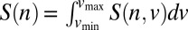. Like Hubbell’s original NTB model, when diversity is large, our models predict log-series SADs under point mutation and multinomial distributions under random fission speciation (Figs. S6 and S7). Using S(n, ν), we can also calculate , the average speciation rate for species with abundance n, and show that it declines as n increases in all our models (Fig. 3 A and B; Figs. S8 and S9). Abundant species are predicted to have low speciation rates, simply because speciation reduces a parent species’ population size by removing the individuals that are transferred to the daughter species. This mechanism is easy to understand for fission speciation but is also remarkably strong for mutation speciation. For example, let f(ν) be the probability density of v for newly produced daughter species with mean and variance . If is small, then is approximately (SI Text)

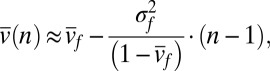and thus the average speciation rate declines with abundance and with a slope that is proportional to the variance of speciation rates among newly born species.

Fig. 3.

Relationships between average speciation rate and abundance (A and B) and between phylogenetic age (generations) and abundance (C and D), predicted by the variable speciation-rate models with mutation speciation (A and C) and random fission speciation (B and D). The trend lines in A were derived analytically for models M_r and M_t and numerically for model M_a; all trends in B–D are moving averages of the mean values. The bins in C are set to 1, 2–100, 101–300, 301–500, 501–700, 701–1,500, and >1,500 and the bins in D are 1–50, 51–100, 101–150, 151–200, 201–300, 301–500, and >500. Other set of bins were also examined and produced the same qualitative patterns. Scatter plots showing all species can be found in Figs. S2–S5. See SI Text for details of calculations.

If sufficiently strong, the negative slope of should cause mean phylogenetic age to increase with n as it is observed to do (Fig. 2A), in contrast to the humped or flat age–abundance relationships predicted by previously published NTB models (Fig. 1 A and B). The reason is that the relatively low speciation rates of abundant species result in relatively long waiting times between daughters. We do not have analytical formulae for the age–abundance relationships, but simulations confirm that mean age is indeed predicted to increase with abundance under fission speciation (Fig. 3). Simulations of models M_r, M_t, and M_a with fission speciation also produce the kind of upper triangular scatter exhibited by the age–abundance data on Panamanian trees (cf. Fig. 2 and Fig. S5). Mutation speciation reduces the strongly negative slope of the age–abundance relationship predicted by M_h and increases the chances that a stochastic simulation will produce a positive slope, although it is not strong enough to make the expected slope consistently positive (Fig. 3; Fig. S10). Using an approximation, we also examined the age–abundance patterns in very large communities over geologic time, which confirmed our findings of a flat relationship in model M_h and positive relationships in models M_r, M_a, and M_t under fission speciation (SI Text; Fig. S11).

Like the original NTB models, the modified NTB models predict log-series distributions of SAD under point mutation and multinomial distributions under random fission speciation (Figs. S6 and S7) when diversity is large. However, compared with the original NTB models, the variable speciation-rate models predict more abundant species and fewer species with intermediate abundance (Figs. S6 and S7). Thus, the new extensions of NTB models explain how the observed age–abundance relationship could be caused by an interaction of macroevolutionary processes and random population drift, without compromising the success of the original NTB models in SAD prediction of species-rich communities.

Previous studies of other groups of species have shown that broad geographic range is sometimes positively correlated with phylogenetic age (35–38). The pattern has been explained outside of the context of NTB, with hypotheses about niches. One hypothesis is that species with unusually broad geographical niches (i.e., broad climate tolerance) will tend to have broad ranges and avoid extinction during climatic fluctuations (39, 40). Another is that species able to attain large ranges might tend to have both broad niches and the ability to disperse over obstacles, which might reduce the rate of allopatric speciation and increase phylogenetic age (41, 42). These hypotheses are also applicable to the age–abundance relationship because total abundance and range are frequently correlated (43).

Collectively, our results provide an alternative hypothesis for the positive correlation between age and abundance, which is more parsimonious than the niche hypotheses. Old phylogenetic ages themselves imply rare speciation, and this is enough to cause the pattern without invoking niche differences. One way to falsify the speciation rate hypothesis would be to produce positive evidence for the mechanisms of the niche hypotheses. For example, one might show that abundant species are indeed ecological generalists, perhaps in common garden experiments, and that the ecological differences among rare and common species are large enough to overwhelm drift.

Our results show how variation among lineages in speciation rates can produce relatively large effects on population sizes, if population dynamics are otherwise neutral. Like many other traits, the rate of speciation is partially conserved within a lineage, but may change over time (29, 30, 32). These two contrary tendencies create variation in speciation rate among different lineages and produces phylogenies in which rapidly speciating lineages have higher species diversity than slowly speciating ones (30). Population dynamics in our model are consistent with the assumptions of NTB in that individuals of all species share the same per capita birth and death probabilities. However, our model differs from the original NTB in the sense that high speciation rates effectively increase realized death rates within a species under fission speciation by a tiny amount, by removing individuals from a species when speciation occurs. Similarly, a high speciation rate reduces a species’ realized birth rate by a tiny amount under mutation speciation. This demographic cost of speciation in our model also makes the community average speciation rate decline through geologic time (34).

Within a lineage, high speciation rates increase species diversity and decrease average phylogenetic age. By splitting the abundance of an ancestral species when speciation occurs, high speciation rates also tend to decrease the average population size within a lineage. Differences in the speciation rate among species thus have population dynamic implications, which are not ecological niches in the traditional sense but which are strong enough to alter the relationship between phylogenetic age and population size. These findings highlight the importance of incorporating population dynamics in macroevolutionary models of speciation and extinction.

Materials and Methods

Plot Data.

A dataset containing 48 plots of tropical tree communities was used to test the relationship between phylogenetic age and species abundance (24, 44, 45). The plots are located in the Panama Canal watershed, which covered a wide range of annual precipitation from 1,760 to 3,750 mm (Fig. S1). Most (45/48) of these plots are 1 ha in area, and three plots are larger than 1 ha, including Barro Colorado Island (BCI; 50 ha), Cocoli (4 ha), and Sherman (5.96 ha). In total, 610 tree size [≥10 cm in breast height diameter (DBH)] species were found in the dataset, including 593 angiosperm species (530 of which were identified to species level and therefore used in the analyses), 1 gymnosperm species (Podocarpus guatemalensis), and 16 unidentified species (24, 44, 45).

Estimating Regional Abundance.

Regional abundance of each species was estimated as a sum of its local abundance from the 45 1-ha plots and 1 random 1-ha subplot from each of the 3 larger plots. For completeness, we constructed 1,200 datasets, using all possible combinations of single hectares from the three plots >1 ha (1,200 = 50 × 4 × 6). The graph in Fig. 2 used the subplots located at the southwest corner of each of the three larger plots, but the results are robust to the choice of the subplots.

Phylogeny.

A tree species list covering the Panama Canal watershed was obtained from the BCI forest dynamics research project (24, 44, 45), and 1,177 angiosperm species from this list had been phylogenetically classified as part of the Angiosperm Phylogeny Group III (APG III) (46) consensus tree. The topology of the phylogeny for these species was obtained with the online program Phylomatic (47), which used a based megatree derived from APG III (46). To estimate the phylogenetic age for each species, we used the module bladj in the software Phylocom version 4.1 to scale branch length using known node ages (48). Here we used the age information from Wikström et al. (49), which estimated divergence times for most angiosperm classes and orders, as well as some families. This two-step approach for constructing a dated phylogeny had been frequently used in recent papers (50–52). Finally, the phylogenetic age is defined by the branch length of the terminal nodes (extant species), which represent the time since the divergence of a species from its closest extant relative.

References

- 1.Hubbell SP. The Unified Neutral Theory of Biodiversity and Biogeography. Princeton, NJ: Princeton Univ Press; 2001. [DOI] [PubMed] [Google Scholar]
- 2.Chisholm RA, Pacala SW. Niche and neutral models predict asymptotically equivalent species abundance distributions in high-diversity ecological communities. Proc Natl Acad Sci USA. 2010;107(36):15821–15825. doi: 10.1073/pnas.1009387107. [DOI] [PMC free article] [PubMed] [Google Scholar]
- 3.Rosindell J, Cornell SJ, Hubbell SP, Etienne RS. Protracted speciation revitalizes the neutral theory of biodiversity. Ecol Lett. 2010;13(6):716–727. doi: 10.1111/j.1461-0248.2010.01463.x. [DOI] [PubMed] [Google Scholar]
- 4.Volkov I, Banavar JR, Hubbell SP, Maritan A. Neutral theory and relative species abundance in ecology. Nature. 2003;424(6952):1035–1037. doi: 10.1038/nature01883. [DOI] [PubMed] [Google Scholar]
- 5.Etienne R, Haegeman B. The neutral theory of biodiversity with random fission speciation. Theoret Ecol. 2011;4(1):87–109. [Google Scholar]
- 6.Hubbell SP. Modes of speciation and the lifespans of species under neutrality: A response to the comment of Robert E. Ricklefs. Oikos. 2003;100(1):193–199. [Google Scholar]
- 7.Etienne R, Apol M, Olff H, Weissing FJ. Modes of speciation and the neutral theory of biodiversity. Oikos. 2007;116(2):241–258. [Google Scholar]
- 8.Volkov I, Banavar JR, Hubbell SP, Maritan A. Patterns of relative species abundance in rainforests and coral reefs. Nature. 2007;450(7166):45–49. doi: 10.1038/nature06197. [DOI] [PubMed] [Google Scholar]
- 9.Fargione J, Brown CS, Tilman D. Community assembly and invasion: An experimental test of neutral versus niche processes. Proc Natl Acad Sci USA. 2003;100(15):8916–8920. doi: 10.1073/pnas.1033107100. [DOI] [PMC free article] [PubMed] [Google Scholar]
- 10.Levine JM, HilleRisLambers J. The importance of niches for the maintenance of species diversity. Nature. 2009;461(7261):254–257. doi: 10.1038/nature08251. [DOI] [PubMed] [Google Scholar]
- 11.Ricklefs RE, Renner SS. Global correlations in tropical tree species richness and abundance reject neutrality. Science. 2012;335(6067):464–467. doi: 10.1126/science.1215182. [DOI] [PubMed] [Google Scholar]
- 12.Turnbull LA, Manley L, Rees M. Niches, rather than neutrality, structure a grassland pioneer guild. Proc Biol Sci. 2005;272(1570):1357–1364. doi: 10.1098/rspb.2005.3084. [DOI] [PMC free article] [PubMed] [Google Scholar]
- 13.Wills C, et al. Nonrandom processes maintain diversity in tropical forests. Science. 2006;311(5760):527–531. doi: 10.1126/science.1117715. [DOI] [PubMed] [Google Scholar]
- 14.Chave J, Muller-Landau HC, Levin SA. Comparing classical community models: theoretical consequences for patterns of diversity. Am Nat. 2002;159(1):1–23. doi: 10.1086/324112. [DOI] [PubMed] [Google Scholar]
- 15.Purves DW, Pacala SW. Ecological drift in niche-structured communities: Neutral pattern does not imply neutral process. In: Burslem D, Pinard M, Hartley S, editors. Biotic Interactions in the Tropics. Cambridge, UK: Cambridge Univ Press; 2005. pp. 107–138. [Google Scholar]
- 16.Tilman D. Niche tradeoffs, neutrality, and community structure: A stochastic theory of resource competition, invasion, and community assembly. Proc Natl Acad Sci USA. 2004;101(30):10854–10861. doi: 10.1073/pnas.0403458101. [DOI] [PMC free article] [PubMed] [Google Scholar]
- 17.Vellend M. Conceptual synthesis in community ecology. Q Rev Biol. 2010;85(2):183–206. doi: 10.1086/652373. [DOI] [PubMed] [Google Scholar]
- 18.Leigh EG., Jr The average lifetime of a population in a varying environment. J Theor Biol. 1981;90(2):213–239. doi: 10.1016/0022-5193(81)90044-8. [DOI] [PubMed] [Google Scholar]
- 19.Ricklefs RE. A comment on Hubbell's zero-sum ecological drift model. Oikos. 2003;100(1):185–192. [Google Scholar]
- 20.Ricklefs RE, Bermingham E. Taxon cycles in the Lesser Antillean avifauna. Ostrich. 1999;70(1):49–59. [Google Scholar]
- 21.Halley JM, Iwasa Y. Neutral theory as a predictor of avifaunal extinctions after habitat loss. Proc Natl Acad Sci USA. 2011;108(6):2316–2321. doi: 10.1073/pnas.1011217108. [DOI] [PMC free article] [PubMed] [Google Scholar]
- 22.Ricklefs RE. The unified neutral theory of biodiversity: Do the numbers add up? Ecology. 2006;87(6):1424–1431. doi: 10.1890/0012-9658(2006)87[1424:tuntob]2.0.co;2. [DOI] [PubMed] [Google Scholar]
- 23.Allen AP, Savage VM. Setting the absolute tempo of biodiversity dynamics. Ecol Lett. 2007;10(7):637–646. doi: 10.1111/j.1461-0248.2007.01057.x. [DOI] [PubMed] [Google Scholar]
- 24.Hubbell SP, et al. Light-Gap disturbances, recruitment limitation, and tree diversity in a neotropical forest. Science. 1999;283(5401):554–557. doi: 10.1126/science.283.5401.554. [DOI] [PubMed] [Google Scholar]
- 25.Cayuela L, Benayas JMR, Justel A, Salas-Rey J. Modelling tree diversity in a highly fragmented tropical montane landscape. Glob Ecol Biogeogr. 2006;15(6):602–613. [Google Scholar]
- 26.Gentry AH. Patterns of neotropical plant species diversity. Evol Biol. 1982;15(1):1–84. [Google Scholar]
- 27.Givnish TJ. On the causes of gradients in tropical tree diversity. J Ecol. 1999;87(2):193–210. [Google Scholar]
- 28.Coyne JA, Orr HA. Speciation. Sunderland, MA: Sinauer Associates; 2004. [Google Scholar]
- 29.Davies TJ, et al. Darwin’s abominable mystery: Insights from a supertree of the angiosperms. Proc Natl Acad Sci USA. 2004;101(7):1904–1909. doi: 10.1073/pnas.0308127100. [DOI] [PMC free article] [PubMed] [Google Scholar]
- 30.Heard SB. Patterns in tree balance with variable and evolving speciation rates. Evolution. 1996;50(6):2141–2148. doi: 10.1111/j.1558-5646.1996.tb03604.x. [DOI] [PubMed] [Google Scholar]
- 31.Magallón S, Sanderson MJ. Absolute diversification rates in angiosperm clades. Evolution. 2001;55(9):1762–1780. doi: 10.1111/j.0014-3820.2001.tb00826.x. [DOI] [PubMed] [Google Scholar]
- 32.Savolainen V, Heard SB, Powell MP, Davies TJ, Mooers AØ. Is cladogenesis heritable? Syst Biol. 2002;51(6):835–843. doi: 10.1080/10635150290102537. [DOI] [PubMed] [Google Scholar]
- 33.Sepkoski JJ., Jr Rates of speciation in the fossil record. Philos Trans R Soc Lond B Biol Sci. 1998;353(1366):315–326. doi: 10.1098/rstb.1998.0212. [DOI] [PMC free article] [PubMed] [Google Scholar]
- 34.Wang S, Chen A, Fang J, Pacala SW. Speciation rates decline through time in individual-based models of speciation and extinction. Am Nat. 2013;182(3):E83–E93. doi: 10.1086/671184. [DOI] [PubMed] [Google Scholar]
- 35.Böhning-Gaese K, Caprano T, van Ewijk K, Veith M. Range size: Disentangling current traits and phylogenetic and biogeographic factors. Am Nat. 2006;167(4):555–567. doi: 10.1086/501078. [DOI] [PubMed] [Google Scholar]
- 36.Jablonski D. Larval ecology and macroevolution of marine invertebrates. Bull Mar Sci. 1986;39(2):565–587. [Google Scholar]
- 37.Paul JR, Tonsor SJ. Explaining geographic range size by species age: A test using Neotropical Piper species. In: Carson WP, Schnitzer S, editors. Tropical Forest Community Ecology. Wiley-Blackwell, Oxford; 2008. pp. 47–62. [Google Scholar]
- 38.Taylor CM, Gotelli NJ. The macroecology of Cyprinella: Correlates of phylogeny, body size, and geographical range. Am Nat. 1994;144(4):549–569. [Google Scholar]
- 39.McKinney ML. Extinction vulnerability and selectivity: Combining ecological and paleontological views. Annu Rev Ecol Syst. 1997;28(1):495–516. [Google Scholar]
- 40.Purvis A, Jones KE, Mace GM. Extinction. Bioessays. 2000;22(12):1123–1133. doi: 10.1002/1521-1878(200012)22:12<1123::AID-BIES10>3.0.CO;2-C. [DOI] [PubMed] [Google Scholar]
- 41.Gaston KJ, Chown SL. Geographic range size and speciation. In: Magurran AE, May RM, editors. Evolution of Biological Diversity. Oxford, UK: Oxford Univ Press; 1999. pp. 237–259. [Google Scholar]
- 42.Jablonski D, Roy K. Geographical range and speciation in fossil and living molluscs. Proc Biol Sci. 2003;270(1513):401–406. doi: 10.1098/rspb.2002.2243. [DOI] [PMC free article] [PubMed] [Google Scholar]
- 43.Brown JH. On the relationship between abundance and distribution of species. Am Nat. 1984;124(2):255–279. [Google Scholar]
- 44.Hubbell SP, Condit R, Foster R. Barro Colorado Forest Census Plot Data. 2005. Available at http://ctfs.arnarb.harvard.edu/webatlas/datasets/bci. Accessed February 2, 2012. [Google Scholar]
- 45. Condit R (1998) Tropical Forest Census Plots (Springer-Verlag and R. G. Landes Company, Berlin)
- 46.Webb CO, Donoghue MJ. Phylomatic: Tree assembly for applied phylogenetics. Mol Ecol Notes. 2005;5(1):181–183. [Google Scholar]
- 47.The Angiosperm Phylogeny Group An update of the Angiosperm Phylogeny Group classification for the orders and families of flowering plants: APG III. Bot J Linn Soc. 2009;161(2):105–121. [Google Scholar]
- 48.Webb CO, Ackerly DD, Kembel SW. Phylocom: Software for the analysis of phylogenetic community structure and trait evolution. Bioinformatics. 2008;24(18):2098–2100. doi: 10.1093/bioinformatics/btn358. [DOI] [PubMed] [Google Scholar]
- 49.Wikström N, Savolainen V, Chase MW. Evolution of the angiosperms: Calibrating the family tree. Proc Biol Sci. 2001;268(1482):2211–2220. doi: 10.1098/rspb.2001.1782. [DOI] [PMC free article] [PubMed] [Google Scholar]
- 50.Cadotte MW, Cardinale BJ, Oakley TH. Evolutionary history and the effect of biodiversity on plant productivity. Proc Natl Acad Sci USA. 2008;105(44):17012–17017. doi: 10.1073/pnas.0805962105. [DOI] [PMC free article] [PubMed] [Google Scholar]
- 51.Kembel SW, Hubbell SP. The phylogenetic structure of a neotropical forest tree community. Ecology. 2006;87(7) Suppl:S86–S99. doi: 10.1890/0012-9658(2006)87[86:tpsoan]2.0.co;2. [DOI] [PubMed] [Google Scholar]
- 52.Liu X, et al. Experimental evidence for a phylogenetic Janzen-Connell effect in a subtropical forest. Ecol Lett. 2012;15(2):111–118. doi: 10.1111/j.1461-0248.2011.01715.x. [DOI] [PubMed] [Google Scholar]
Associated Data
This section collects any data citations, data availability statements, or supplementary materials included in this article.