

Abstract
Using large-sample theory, we present a unified approach to power calculations for family-based association tests. Currently available methods for power calculations are restricted to special designs or require approximations or simulations. Our analytical approach to power calculations is broadly applicable in many settings. We discuss power calculations for two scenarios that have high practical relevance and in which power previously could only be assessed by simulation studies or by approximations: (1) studies using both affected and unaffected offspring and (2) studies with missing parental information. When the population prevalence is high, it can be worthwhile to genotype unaffected offspring. For many scenarios, high power can be achieved with reasonable sample sizes, even when no parental information is available.
Introduction
In this article, we address power calculations for generalized family-based association tests (FBATs) (Laird et al. 2000; Rabinowitz and Laird 2000). We use the term “FBAT” to denote a genetic-association test that uses genetic data on family members to compute the distribution of a suitable test statistic under the null hypothesis, conditioning on the phenotypes. Examples are given below. FBATs are powerful tests for detecting linkage between a marker and a disease-susceptibility locus in the presence of linkage disequilibrium between the two loci. The best known FBAT is the transmission/disequilibrium test (TDT) (Ott 1989; Spielman et al. 1993); it was designed for the special setting of sampling affected individuals and their parents, where parents' genotypes are available. However, many genetic studies have missing parents, affected and unaffected offspring, continuous phenotypes, and/or multiple phenotypes. A variety of approaches have been proposed to deal with these issues; for reviews, see Zhao (2000) or Schulze and McMahon (2002). Most research has focused on the distribution of the proposed test statistics under the null hypothesis and has assessed the achieved power of the proposed tests either by simulation studies (Risch 2000; Horvath et al. 2001; Q. Yang, X. Xu, and N. M. Laird, unpublished data) or by approximations (Whittaker and Lewis 1998).
For “simple” scenarios (i.e., trios or trios with one additional offspring), Knapp (1999a) and Chen and Deng (2001) computed the power by deriving the expected value of the test statistic under the alternative hypothesis and then computing the power of the expected statistic. In contrast with that, we compute the expected power of the actual test statistic. First, we obtain the power of the test statistic, conditional on the phenotypes and mating types. Then, we integrate the conditional power over the phenotypes and mating types, to obtain the expected power. Since we are able to compute the conditional power for virtually any scenario (e.g., multiple offspring, missing parental information, etc.), and since integrating over the data can always be solved numerically, our approach to power calculation can be applied much more generally. The approach is broadly applicable to multiallelic loci, continuous traits, and/or multivariate phenotypes (Lange et al., in press). Here, we will discuss only the situation in which we observe one dichotomous trait; continuous traits will be discussed in a separate article.
To illustrate the generality of our new approach, we compare power results obtained by our approach with those of both Knapp (1999a) and Whittaker and Lewis (1998). Our approach and Knapp’s agree well in the case in which Knapp’s has been applied. Since Whittaker and Lewis (1998) derived their results under the assumption that the alternative hypothesis would be very close to the null hypothesis, the two approaches demonstrate perfect agreement when the alternative hypotheses are indeed close to the null hypothesis. However, when the alternative hypotheses are far away from the null hypothesis, the Whittaker and Lewis (1998) method becomes less reliable. In addition, we will present power calculations for situations in which the parental genotypes are missing, but additional offspring are available.
In our section on “Notation and Power Calculations,” we discuss how the unconditional/expected power can be computed. In the following section, on “Computation of the Conditional Marker Distribution and the Conditional Family-Type Distribution,” we derive the conditional probabilities required for the computation of the unconditional power. Our approach is generally applicable and can handle a variety of different scenarios—for example, multiple offspring, multiple phenotypes, missing parental information, and environmental effects. Our “Results” section shows power calculations for scenarios in which additional offspring are given and/or parental genotypic information is missing. Finally, in our section on “Application to Study Design,” we use our approach to power calculations to design a study for bipolar disorder.
Notation and Power Calculations
For simplicity of exposition, we assume that we observe a biallelic marker with alleles A and B. The disease penetrances for 0, 1, or 2 disease alleles are f0, f1, and f2, respectively. We denote the allele frequency of the disease gene by p, the population prevalence of the disease by K, and the fraction of the disease attributable to carrying at least one copy of the disease gene by AF—that is, AF=(K-f0)/K. Like Risch and Merikangas (1996), Camp (1997), Knapp (1999a) and Whittaker and Lewis (1998), we assume the best-case scenario for the marker locus—that is, that the marker locus is the disease locus and that, hence, the A allele frequency is p.
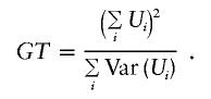
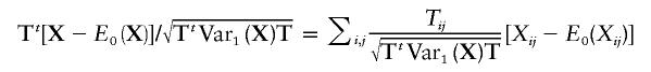
Furthermore, there are n independent families, and the ith family has mi offspring. We denote the marker score for jth offspring in the ith family by Xij. The total number of marker scores Xij,j=1,…,mi;i=1,…,n is N. Note that the actual coding of the marker score depends on the assumed genetic model. The corresponding trait information is given by Yij, where affected offspring are coded by Yij=1, unaffected offspring by Yij=0, and offspring with unknown phenotype by Yij=NA. When parental genotypic information for the ith family is recorded, it is denoted by Pi1 and Pi2. For biallelic markers, the possible values of Pi1 and Pi2 can be characterized as 0, 1, or 2 for the number of target alleles. Laird et al. (2000) then defined the generalized FBAT statistic by
 |
In this equation,  ,
,  , and Tij an appropriate coding of the phenotype Yij. E0(Xij) is the expected marker score under the null hypothesis and
  is the marker covariance under the null hypothesis. When the phenotype is missing (i.e., when Yij=NA), we set Tij=0. When both parents are observed, setting Tij=yij gives the TDT discussed by Spielman et al. (1993), which is based on affected (yij=1) offspring only. Setting Tij=yij-z, with a constant offset z,0<z<1, defines the TDT proposed by Whittaker and Lewis (1998), which includes unaffected offspring in the computation of the test statistic. When both parents are observed, the marker means and covariances under the null hypothesis, E0(Xij) and
  , are computed conditional on the parental genotypes, Pi1 and Pi2, where the transmission probabilities are defined by Mendelian laws.
When parents are missing, the RC-TDT (Knapp 1999b), S-TDT (Spielman and Ewens 1998), and FBAT (Laird et al. 2000; Rabinowitz and Laird 2000) use alternative conditions for the computation of the marker means and covariances under the null hypothesis (e.g., the minimal sibship condition for S-TDT or the R-condition for RC-TDT). These conditions are based on suitable sets of available genetic information within one family and the observed phenotypes. Loosely speaking and without loss of generality, any of those conditions can be understood as a function of offspring genotypes and available parental genotypes that is held constant when E0(Xij) and  are computed. We will denote these conditions by Si. Although the methodology proposed here is valid for all conditions addressed by RC-TDT, S-TDT, and FBAT, we will use the FBAT condition in all our examples. For FBAT, Si is the minimal sufficient statistic for the parental genotypes (Rabinowitz and Laird 2000).
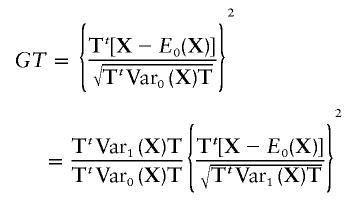
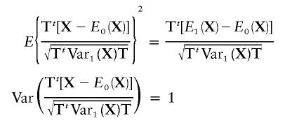
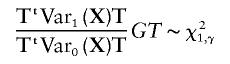
Standard asymptotic theory implies that, under the null hypothesis and given the phenotypes Y=(Y11,…,Ynmn) and the condition S=(S1,…,Sn), GT is χ2 distributed with 1 df—that is,
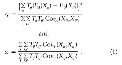
When the marker means EA(Xij) and (co)variances  are given under the alternative hypothesis, the distribution of GT under the alternative hypothesis can be computed by a scaled, noncentral χ2 distribution: ωGT∼χ21,γ, with
 |
The proof of this result is shown in appendix A. The extension of the conditional power formula (1) to multiallelic loci can be found in the work of Lange and Laird (in press). In this setup, the conditional power of GT for the significance level α is given by
It is important to note that, since E0(.), EA(.),  and
and  are computed conditional on Y and S, formula (2) can not be used directly when the phenotypes Y and the data defining S are not observed. Y and S have to be integrated out to obtain the unconditional/expected power—that is,
where 𝒜 is the ascertainment condition for the phenotype Y. We make the assumption that the ascertainment condition depends only on the phenotype Y and the expectation is over the distribution of Y,S∣𝒜, but the approach can be extended so that 𝒜 depends on the phenotypes of the parents. Thus, the second stage of computing the unconditional/expected power involves the conditional distribution of the family types  under the alternative hypothesis. Since yi,si are discrete and bounded random variables, (3) can be written as a finite sum:
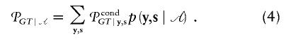 |
Hence, 𝒫GT∣𝒜 can always be computed by direct evaluation of each possible term in the summation. In appendix B, we describe technical details that accelerate the computation of (4).
When the power function in the unconditional/expected power formula (3) is approximated by a first-order Taylor expansion in Y and S—that is, by E[Power(FBAT)]≗Power[E(FBAT)]—the approach of Knapp (1999a) is obtained. In full generality, the Lagrange term in the Taylor approximation—and, therefore, the accuracy of Knapp’s approach (1999a)—will depend on the second moment expressions of S and the phenotypes Y, which are not fixed by the ascertainment condition. Since all phenotypes are fixed at 1 in the scenarios considered by Knapp (1999a), and, since the parental genotypes are observed, S=(P1,P2), the approximation error is minimal. However, when not all phenotypes are defined by the ascertainment condition (e.g., only the first offspring must be affected) and S becomes more complex (e.g., parental genotypic information is missing), the approximation error can become considerably larger.
Although the numerical differences we found between our approach and Knapp’s were usually not noteworthy for the scenarios considered by Knapp (1999a) and Chen and Deng (2001), the theoretical advantages of our methodology are of practical relevance. Since the direct computation of the unconditional mean and variance of GT∣Y,S is already rather difficult for the scenarios considered in Knapp (1999a), and since approximations have to be utilized (Knapp 1999a), potential extensions to more-realistic scenarios become even more complex (Chen and Deng 2001). On the other hand, the methodology proposed here can easily be applied to complex scenarios (e.g., missing parental genotypes and multiple continuous phenotypes per offspring). Result (1) for conditional power calculations allows us to compute the conditional power for any scenario, as long as we are able to derive the conditional marker distribution under the alternative hypothesis. In the next section (formula [5]), we show that this can be done for virtually any scenario. Then the second step, “unconditioning” the conditional power, can be achieved numerically at all times, either by numerical summation, numerical integration, Monte Carlo simulation, or Markov chain–Monte Carlo (MCMC) methods.
Note that, when numerical integration/summation is not feasible, computing the sum by Monte Carlo simulations or MCMC is more efficient than assessing the power by simulations. In a pure simulation experiment, the test result is either significant or not significant, which means that we are looking at a discrete variable that can either be 1 or 0. However, when Monte Carlo simulation is used for the computation of the sum in (4), the variable of interest is the conditional power, which is a continuous variable between 0 and 1. It is obvious that a continuous variable contains more information and has less variance than a discrete variable. A pure simulation study will therefore require far more replicates than computing the sum of the conditional power by Monte Carlo simulation. Finally, we note that Knapp (1999a) and Chen and Deng (2001) compute an approximation to the power of the ”expected” test statistic rather than the expected power of the actual test statistic.
Computation of the Conditional Marker Distribution and the Conditional Family-Type Distribution
In this section, we discuss the computation of the conditional marker distribution under both hypotheses and the conditional distribution of the family types (i.e., yi and si) under the alternative hypothesis. Although the conditional marker distribution is required in the conditional power calculation for the scaling parameter ω and the noncentrality parameter γ, the distribution of the family types conditional on the ascertainment condition is needed to integrate out these variables in (3) to and obtain the unconditional/expected power.
Since we assume independence of the families, it is sufficient to discuss the marker distribution within one family. The conditional marker distribution  can be derived by repeated application of Bayes's theorem and is given, under the null and alternative hypotheses, by
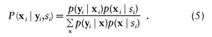 |
When the marker locus and the disease locus are not the same, the probability of the disease locus gi, given the marker locus xi, has to be computed, by p(gi∣xi). Then p(yi∣xi) in (5) is replaced by  .
.
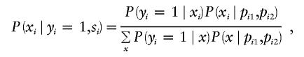
The probability p(xi∣si) can be computed under both hypotheses by repeated application of Bayes's theorem. Under the null hypothesis, note that  does not depend on the marker score and (5) simplifies to
  , which will not depend upon model assumptions and population parameters (appendix I in Rabinowitz and Laird 2000). Nevertheless formula (5) is of practical relevance also under the null hypothesis, since it provides a standardized way for the computation of the conditional marker distribution that can easily be implemented in a software package, e.g. when either one or both parents are missing it can be used as an alternative algorithm to compute the conditional marker distribution given in Rabinowitz and Laird (2000).
When trios with one offspring are ascertained, mi=1, and the parental genotypes are observed, the sufficient statistic Si is given by pi1,pi2 and the conditional marker distribution for the TDT by Spielman and Ewens (1998) can be obtained by direct application of formula (5),
 |
where  is over all possible values of xi, given pi1 and pi2; it depends on the marker coding, as well as on pi1 and pi2. The probability
  is given by Mendelian law under both H0 and HA. The conditional distribution
  is given, under the null hypothesis, by
where K is the disease prevalence and under the alternative hypothesis by
where f0, f1, and f2 are the penetrances of the underlying disease model. The application of formula (5) to more complex scenarios (e.g., multiple offspring and missing parental information) will be discussed in our “Results” section.
The computation of the distribution of the family type  , given 𝒜, is done in a similar way. The ascertainment condition 𝒜 describes how offspring are sampled from the total population on the basis of their phenotypes. For example, for the TDT proposed by Spielman and Ewens (1998), the ascertainment condition is given by
  , which means that only affected offspring are used in the test. Given the ascertainment condition 𝒜, the conditional distribution of
  can be computed by
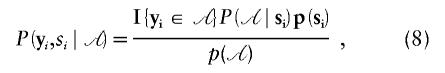 |
with  for yi∈𝒜 and
  otherwise. As for the conditional marker distribution, probabilities
  ,
,  , and p(si) can be computed, under the alternative hypothesis, by repeated application of Bayes's theorem. All technical details for the computation of the conditional probability are included in a technical report that is available on our Web page.
Results
In this section, we discuss two power-calculation scenarios, additional offspring and missing parental information; both scenarios are highly relevant to association studies. Many diseases considered in association studies have late onset (e.g., Alzheimer disease), and so genotyping the parents is not feasible. However, it might be relatively easy to sample siblings.
Application I: Power When Both Parents Are Available and One Additional Unaffected Offspring Is Included
In this section, we compute the power of the FBAT for affected trios with one additional unaffected sibling (mij=2) and examine the influence of weighting scheme on the power. We will also compare our results with those of Whittaker and Lewis (1998). Whittaker and Lewis (1998) suggested including the unaffected offspring by use of the coding Tij=yij-z, where z=K is the disease prevalence. Since K is not known, in general, we examine the power of FBAT as a function of z.
We use formula (5) to derive the joint conditional distribution of the marker scores xi1 and xi2. All phenotypes are fixed by the ascertainment condition 𝒜—that is,  —and the parental genotypes are known. Hence, the minimal sufficient statistic of FBAT depends only on the parental genotypes—that is, si=(pi1,pi2). The conditional marker distribution is given by
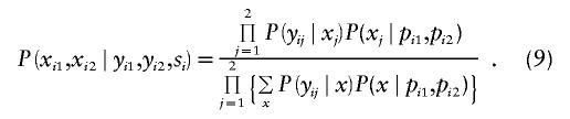 |
Note that we assume independence of Yij∣Xj and of Xj∣(Pi1,Pi2) in (9). In principle, a more general model can be used that allows for nonindependence of the values of Yij∣Xj, as in the work of Q. Yang, X. Xu, and N. M. Laird (unpublished data). Whereas P(x∣pi1,pi2) depends only on Mendelian transmission,  depends on the hypothesis and the underlying genetic model. Under the null hypothesis, it is given by (6) and under the alternative hypothesis by (7).
Under the assumption of an additive coding for the marker scores (i.e., xij=0,1,2), there are 32=9 possible combinations for Si=(pi1,pi2), which we will denote here by S(1),…,S(9). Further, the number of observed S(k) is given by nk (i.e.,  ). Then, the scaling parameter ω for the conditional power formula (2) can be computed by
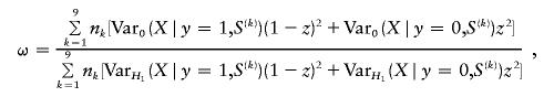 |
and the noncentrality parameter γ can be computed by
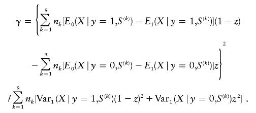 |
Further, we use formula (8) to compute the distribution of S(k) conditional on the ascertainment condition 𝒜, which is given here by  . Having these conditional distributions, it is straightforward to compute the unconditional/expected power.
To compare our results with those of Whittaker and Lewis (1998), we assume a multiplicative model,  . Under the assumption that the alternative hypothesis would be close to the null hypothesis (low gene effect)—that is,
Whittaker and Lewis (1998) suggested that inclusion of unaffected siblings gives maximum power when the offset z is chosen to be the disease prevalence and that the power gained by inclusion of unaffected offspring does not outweigh the cost of the additional genotyping. For alternative hypotheses satisfying the assumption of low gene effects, our power calculations, as well as methods discussed elsewhere (Q. Yang, X. Xu, and N. M. Laird, unpublished data), confirm the finding of Whittaker and Lewis (1998).
However, when we consider scenarios like those discussed by Boehnke and Langefeld (1998) and Knapp (1999a), in which the authors assume that  is in the range 1.5–4, and in which unaffected siblings are included, we observe, for common diseases, a substantial gain in power over the standard TDT, which uses only affected. For
  these results are illustrated for a common and a rare disease in figure 1. Figure 1 strongly suggests that genotyping unaffected offspring can be worthwhile for common diseases, as shown elsewhere (Q. Yang, X. Xu, and N. M. Laird, unpublished data). Furthermore, it is important to note that, in any case, z>0 is a better choice than the standard TDT. However, the power is relatively insensitive to the choice of the offset z in a limited range around the prevalence. When
  is in the range 1.5–4, our analytical power calculations show that the optimal FBAT is obtained when the offset z is chosen to be greater than the disease prevalence, although the amount of power gained over use of z as “disease prevalence” is very small.
Figure 1.

Power of FBAT test for trios with one additional unaffected offspring and both parents' genotypes observed. The dotted line shows the power of the standard TDT, including only the affected offspring. The vertical line shows the location of the disease prevalence K. a, Multiplicative model for a common disease: disease prevalence K=0.3, allele frequency of the disease gene p=0.143, fraction of the disease attributable to carrying at least one disease gene AF=0.25, significance level α=0.01, and sample size 100. Optimal offset choice z=0.4. Power gain by optimal choice of z over z=0 is 25%. b, Multiplicative model for a rare disease: disease prevalence K=0.05, allele frequency of the disease gene p=0.05, fraction of the disease attributable to carrying at least one disease gene AF=0.3, significance level α=10-4, and sample sizes 100. Optimal choice of z=0.15. Power gain by optimal choice of z over z=0 is 5%.
Power of FBATs When Both Parental Genotypes Are Missing
Since the standard TDT discussed by Spielman et al. (1993) requires the parental genotypes, a variety of extensions have been proposed when either one or both parents are missing: SDT by Horvath and Laird (1998), S-TDT by Spielman and Ewens (1998), RC-TDT by Knapp (1999b), and FBAT by Rabinowitz and Laird (2000). The advantage of the FBAT approach is its flexibility; it can handle scenarios with one missing parent, arbitrary numbers of offspring within a family, etc. We will therefore concentrate here on power calculations for FBATs. However, for many scenarios, RD-TDT and FBAT give similar results (Horvath et al. 2001).
For simplicity, we examine only scenarios where both parents are missing. We assume that we observe at least two offspring per family (mi⩾2). The sufficient statistic Si(xi) is given in Rabinowitz and Laird (2000) and can be used directly in formula (5) to derive the conditional marker distribution for FBATs under the null and alternative hypothesis.
Having these conditional distributions, the conditional marker mean and variance can be calculated under the null and alternative hypothesis (formula [5]). Then, the scaling parameter ω and the noncentrality parameter γ in the conditional power formula (2) can be computed as in our section on “Application I.” In the ”unconditioning” step, we assume that families are ascertained with at least one affected offspring—that is,  . The probability p(yi,si∣𝒜) is obtained by application of formula (8).
We compute the power of GT and its dependence on the offset z for a variety of sampling plans assuming parental genotype data are always missing. We assume that the penetrances under the alternative model are given by a multiplicative model. Figure 2 shows the results of the asymptotic power calculations outlined above for common and rare disease scenarios. To study the effect of missing parental information on the power, we also give the power of GT for the same number of offspring when the parental genotypes are known.
Figure 2.

Power of FBAT tests for multiplicative models: Significance level α=0.01. The numbers shown above the graphs correspond to the numbers of genotyped subjects in each family. a, n=200, p=0.2, K=0.3, AF=0.2. b, n=100, p=0.05, K=0.2, AF=0.2. c, n=100, p=0.05, K=0.05, AF=0.2. d, n=200, p=0.2, K=0.05, AF=0.3.
As expected, the loss of power caused by missing parental information decreases with increasing family size. While the loss of power for two siblings with no parental information is relatively large compared to the power when both parents are given, the loss of power is moderate for the families with 3 siblings. In fact, for K⩾0.2, the power of the three sibling design is indistinguishable from the ”two-parent and two-offspring” design, and should be preferred as it requires less genotyping and has less sensitivity to z.
For all tests, choosing z to be the disease prevalence seems to be a reasonable choice. However, the choice of z has only a minor affect on the power of all tests as long as z is in a sensible range around the disease prevalence. For rare diseases, z=0 is a reasonable choice, which corresponds to treating the phenotypes of the unaffected siblings as unknown. When trios with one affected offspring or two offspring without parental information are given, there is no dependence on the offset z. Although this observation is trivial for affected trios, it is unexpected for two offspring with no parental information. In this case, it can be explained by the definition of the sufficient statistic. Since the sufficient statistic conditions on the observed marker scores, the correlation between the two marker scores is always −1 when only two offspring without parental information are given. This simplifies the formulas for the scaling parameter ω and the noncentrality parameter γ, so that they do not depend upon the offset. One might also get the impression that the power does not depend on the offset for three offspring and no parental information. However, this impression is due to the selected offset range between 0.0 and 0.6 in figure 2. For offsets between 0.6 and 1.0, the power also depends on the offset choice for this family type.
Application to Study Design
An ancillary genetic study of bipolar disorder is being planned that builds on patients enrolled in a large ongoing clinical trial. For illustration, we assume that 1,003 families with one affected proband will participate in the study: 213 probands with both parents, 175 probands with one parent and one sibling, 175 probands with one parent and two siblings, 220 probands with one sibling, and 220 probands with two siblings. Because of cost and recruitment considerations, siblings will not be phenotyped. With low disease prevalence (K≗0.01), this should not have a substantial impact on the power, but this can be tested using our method. We compare power under the assumptions that siblings are phenotyped or not, for a fixed set of penetrance functions and a range of allele frequencies that give K≗0.01. For the case when the siblings are phenotyped, we set the offset to 0.01. Furthermore, we assume that the significance level is α=0.00001. The achieved power for a range of potential allele frequencies is shown in table 1 when the sibling are phenotyped or not. Table 1 shows that phenotyping additional offspring has virtually no effect on the achieved power and therefore is not worthwhile in this study.
Table 1.
Power for Bipolar Disorder Study[Note]
|
Power |
||
| p | Additional OffspringPhenotyped | Additional OffspringNot Phenotyped |
| .5 | .989 | .986 |
| .4 | .997 | .995 |
| .3 | .998 | .997 |
| .2 | .994 | .993 |
| .1 | .911 | .902 |
| .05 | .488 | .474 |
| .01 | .007 | .007 |
Note.— Significance level α=0.00001, and penetrance function fAA=0.03, fAB=0.02, and fBB=0.01.
Discussion
In this study, we have presented an approach to power calculations for FBATs. Our approach differs from the approach taken by Knapp (1999a) and its extension in the sense that it computes the expected power of the actual test statistic, whereas Knapp’s approach gives the power of the expected statistic. Although the results of the two approaches do not differ greatly for the examples considered in the literature, the difference becomes relevant when the family size becomes larger, when parental information is missing, or when extensions to continuous traits are considered. For all these scenarios, the power has so far been assessed by simulation experiments. Our approach allows the computation of the unconditional/expected power for these scenarios and thereby becomes an important tool for the design of genetic studies (e.g., comparisons of sample designs in terms of genotyping and prevalence). For discordant sibships, we applied our approach to verify the results obtained by the approximation proposed by Whittaker and Lewis (1998). Although we found that offset choices close to the population prevalence are not always optimal, they seem to be a reasonable rule of thumb. Further, genotyping of unaffected offspring can be beneficial when the population prevalence is high.
We discussed design issues and powerful offset choices for situations in which no parental information is available. For many scenarios, high power can be achieved with a reasonable sample size in the absence of parental information. In these situations, the influence of the offset on the power is negligible.
The methodology proposed here is fully general; hence, extensions to sampling designs and power calculations for multiallelic loci and continuous phenotypes are straightforward. We have implemented our approach to power calculations in a software package called “PBAT,” which is available on our Web page. In addition to the scenarios discussed here, PBAT can also be used for power calculations for continuous traits and when marker locus and disease locus are not identical.
Acknowledgments
We would like to thank Dr. Ed Silverman for his helpful comments on an earlier version of the paper. This research was supported in part by grants MH59532 and HL66383 from the National Institutes of Health. The Childhood Asthma Management Program (CAMP) is supported by contracts from the National Heart, Lung and Blood Institute, including N01 HR16040. We acknowledge the CAMP investigators and research team for assistance in collection of the CAMP Genetics Ancillary Study data. Comments from three referees were very helpful in preparing this version of the paper.
Appendix A : Asymptotic Distribution of GT under the Alternative Hypothesis
We denote the vector containing all marker information by
and the corresponding vector of the coded trait information by  . Then, the statistic GT can be written as
 |
Under the alternative hypothesis, note that
 |
Furthermore,
 |
is a weighted sum of potentially dependent random variables. However, since we assume that the families are independent and that the family size is bounded, we can rewrite  as a sum of independent sub-sums—that is,
where Zi is computed on the basis of the data of the ith family. The values of Zi are therefore independent. We standardize the weighted sum (A2) by its variance  and can then apply standard asymptotic theory to
  . The asymptotic distribution of
  under the alternative hypothesis is, therefore, given by a noncentral χ2 distribution with 1 df and noncentrality parameter
  . Thus, under the alternative hypothesis,
 |
Appendix B
We refer to each combination of possible values for yi and si as a “family type,” denoted by the vector qk=(y,s),k=1,…,FT, where FT is the number of possible family types. If we define an n-dimensional unit vector by  , it is easy to see that
where pMultinomial(π1,…,πFT)(n1,…,nFT) is the density of the multinomial distribution with probabilities π1,…,πFT. The π1,…,πFT are defined by  . Therefore, it is always possible to compute the exact unconditional power of GT by numerical integration of (B1). In situations with many potential family types qk (e.g., either families with many offspring or offspring with many traits), this numerical integration may be very time consuming and can be replaced either by Monte Carlo simulations or by MCMC methods. However, for the situations considered in this study, the numerical computation of the sum is feasible.
For many scenarios, the number of family types can be reduced. For example, when the phenotypes are fixed by the ascertainment condition (e.g., y=1 in the work of Spielman et al. [1993] or y1=1 and y2=0 in the work of Whittaker and Lewis [1998]), and when the parental genotypes are observed, the family types are defined by the observed parental information. For simplicity of exposition, assume an additive marker coding. When the scaling parameter ω and the noncentrality parameter δ are computed for the conditional power formula (2), it is easy to see that q=(p1,p2)=(0,0),(0,2),(2,0) and (2,2) are noninformative and do not contribute to the scaling parameter ω and the noncentrality parameter δ. Further, it is important to note that q=(0,1) and q=(1,0) make the same contribution to ω and δ. The same is true for q=(0,2) and q=(2,0). In this setup, therefore, it is possible to reduce the number of family types to four distinct types—(0,1), (1,1), (1,2) and ”noninformative”—and to change the probabilities πi appropriately. This reduction of the number of family types accelerates the computation of the unconditional power substantially.
Electronic-Database Information
Accession numbers and URLs for data presented herein are as follows:
- FBAT Web page, http://www.biostat.harvard.edu/~fbat/default.html (for PBAT software package)
References
- Boehnke M, Langefeld CD (1998) Genetic association mapping based on discordant sib pairs: the discordant-alleles test. Am J Hum Genet 62:950–961 [DOI] [PMC free article] [PubMed] [Google Scholar]
- Camp NJ (1997) Genomewide transmission/disequilibrium testing—consideration of the genotypic relative risks at disease loci. Am J Hum Genet 61:1424–1430 [DOI] [PMC free article] [PubMed] [Google Scholar]
- Chen W-M, Deng H-W (2001) A general and accurate approach for computing the statistical power of the transmission disequilibrium test for complex disease genes. Genet Epidemiol 21:53–67 [DOI] [PubMed] [Google Scholar]
- Horvath S, Laird NM (1998) A discordant-sibship test for disequilibrium and linkage: no need for parental data. Am J Hum Genet 63:1886–1897 [DOI] [PMC free article] [PubMed] [Google Scholar]
- Horvath S, Xu X, Laird NM (2001) The family based association test method: strategies for studying general genotype-phenotype associations. Eur J Hum Genet 9:301–306 [DOI] [PubMed] [Google Scholar]
- Knapp M (1999a) A note on power approximations for the transmission/disequilibrium test. Am J Hum Genet 64:1177–1185 [DOI] [PMC free article] [PubMed] [Google Scholar]
- Knapp M (1999b) Using exact P values to compare the power between the reconstruction-combined transmission/disequilibrium test and the sib transmission/disequilibrium test. Am J Hum Genet 65:1208–1210 [DOI] [PMC free article] [PubMed] [Google Scholar]
- Laird NM, Horvath S, Xu X (2000) Implementing a unified approach to family based tests of associaton. Genet Epidemiol Suppl 19:S36–S42 [DOI] [PubMed] [Google Scholar]
- Lange C, Laird NM (2002) On a general class of conditional tests for family-based association studies in genetics: the asymptotic distribution, the conditional power and optimality considerations. Genet Epidemiol 23:1–16 [DOI] [PubMed] [Google Scholar]
- Lange C, Silverman EK, Xu X, Weiss ST, Laird NM. A multivariate transmission disequilibrium test: FBAT-GEE. Biostatistics (in press) [DOI] [PubMed] [Google Scholar]
- Ott J (1989) Statistical properties of the haplotype relative risk. Genet Epidemiol 6:127–130 [DOI] [PubMed] [Google Scholar]
- Risch N (2000) Searching for genetic determinants in the new millennium. Nature 405:847–856 [DOI] [PubMed] [Google Scholar]
- Rabinowitz D, Laird NM (2000) A unified approach to adjusting association tests for population admixture with arbitrary pedigree structure and arbitrary missing marker information. Hum Hered 50:211–223 [DOI] [PubMed] [Google Scholar]
- Risch N, Merikangas K (1996) The future of genetic studies of complex human diseases. Science 273:1516–1517 [DOI] [PubMed] [Google Scholar]
- Spielman RS, Ewens WJ (1998) A sibship test for linkage in the presence of association. Am J Hum Genet 62:450–458 [DOI] [PMC free article] [PubMed] [Google Scholar]
- Schulze TG, McMahon FJ (2002) Genetic association mapping at the crossroads: which test and why? Overview and practical guidelines. Am J Med Genet 114:1–11 [DOI] [PubMed] [Google Scholar]
- Spielman RS, McGinnis RE, Ewens WJ (1993) Transmission test for linkage disequilibrium: the insulin gene region and insulin-dependent diabetes mellitus (IDDM). Am J Hum Genet 52:506–516 [PMC free article] [PubMed] [Google Scholar]
- Whittaker JC, Lewis CM (1998) Power comparisons of the transmission/disequilibrium test and sib–transmission/disequilibrium-test statistics. Am J Hum Genet 65:578–580 [DOI] [PMC free article] [PubMed] [Google Scholar]
- Zhao H (2000) Family-based association studies. Stat Methods Med Res 9:563–587 [DOI] [PubMed] [Google Scholar]