

Abstract
EEG‐fMRI in epileptic patients is commonly analyzed using the general linear model (GLM), which assumes a known hemodynamic response function (HRF) to epileptic spikes in the EEG. In contrast, independent component analysis (ICA) can extract Blood‐Oxygenation Level Dependent (BOLD) responses without imposing constraints on the HRF. This technique was evaluated on data generated by superimposing artificial responses on real background fMRI signals. Simulations were run using a wide range of EEG spiking rates, HRF amplitudes, and activation regions. The data were decomposed by spatial ICA into independent components. A deconvolution method then identified component time courses significantly related to the simulated spikes, without constraining the shape of the HRF. Components matching the simulated activation regions (“concordant components”) were found in 84.4% of simulations, while components at discordant locations were found in 12.2% of simulations. These false activations were often related to large artifacts that coincidentally occurred simultaneously with some of the random simulated spikes. The performance of the method depended closely on the simulation parameters; when the number of spikes was low, concordant components could only be identified when HRF amplitudes were large. Although ICA did not depend on the shape of the HRF, data processed with the GLM did not reveal the appropriate activation region when the HRF varied slightly from the canonical shape used in the model. ICA may thus be able to extract BOLD responses from EEG‐fMRI data in epileptic patients, in a way that is robust to uncertainty and variability in the shape of the HRF. Hum Brain Mapp, 2009. © 2008 Wiley‐Liss, Inc.
Keywords: independent component analysis, EEG‐fMRI, epilepsy, deconvolution, hemodynamic response function
INTRODUCTION
Simultaneous electroencephalographic (EEG) and functional magnetic resonance imaging (fMRI) recordings have shown promise in the study of epilepsy. This noninvasive technique can locate significant Blood‐Oxygenation Level Dependent (BOLD) responses to epileptiform discharges measured on the EEG. Several studies [Aghakhani et al.,2006; Al Asmi et al.,2003; Federico et al.,2005; Salek‐Haddadi et al.,2006] have reported cases where the EEG‐fMRI localization was consistent with other clinical data. However, there were also a large proportion of investigated patients who did not show significant BOLD responses to interictal spikes. In the large majority of studies, the fMRI data were processed using the general linear model (GLM) framework [Worsley and Friston,1995; Worsley et al.,2002], which requires a model of the hemodynamic response function (HRF) to identify voxels significantly correlated with the model time course.
It has been suggested that the absence of significant BOLD responses may be partially explained by a mis‐specification of the model [Bagshaw et al.,2004; Lemieux et al.,2008; Lu et al.,2006]. Typically, a canonical HRF based on the BOLD response to brief auditory stimuli [Glover,1999] is used, although this shape may be altered for interictal spikes [Benar et al.,2002]. The HRF may show variability for different types of epileptiform discharges, between subjects, across brain regions, and even across sessions for the same subject [Aguirre et al.,1998; Handwerker et al.,2004; Menz et al.,2006]. Moreover, even if the HRF shape is specified correctly, there is evidence that the linearity of the model may not hold, especially if the events of interest are closely spaced in time [Friston et al.,1998; Jacobs et al.,2008].
Independent component analysis (ICA) is a data‐driven method that has recently found applications in the study of fMRI data [McKeown et al.,1998]. ICA can be used in an exploratory manner to detect consistent patterns of brain activation with a common fMRI time course. A large number of such components may be identified, after which it becomes necessary to reliably recognize the components that represent activity relevant to the task under investigation. Nevertheless, the attractiveness of ICA lies in its lack of use of any strong assumptions on the data. Unlike approaches based on the GLM, ICA methods do not impose constraints on the shape of the HRF. ICA may thus detect responses that would otherwise be ignored by a model‐based framework. Moreover, ICA has shown the ability to isolate sources of structured noise that may otherwise be too complex to model as confounds in the multiple regression framework of the GLM [Thomas et al.,2002].
In the context of epileptiform discharges, the uncertainty surrounding the shape of the HRF and the validity of the model naturally suggests the use of a data‐driven method for analysis of the fMRI data acquired from epileptic patients. A study on patients, whose GLM activations were concordant with other clinical data, revealed that ICA could also identify similar brain areas [Rodionov et al.,2007]. This study used an automated classification procedure [De Martino et al.,2007] to discard components representing fMRI artifacts (scanner noise, motion, physiological artifacts). Components related to the epileptic activity were then identified by a combination of visual inspection, overlap of the component spatial maps with the GLM activation, and correlation of the component time course with the model used in the GLM analysis. Therefore, the component selection still depended on the canonical HRF used in the GLM. The purpose of the current study was to develop an ICA framework to identify BOLD responses to epileptiform discharges, in a way that is independent of the shape of the HRF. However, validation of such methods can be very difficult due to the absence of a gold standard with which to corroborate the results. Consequently, the method was applied to simulated BOLD changes in real simultaneous EEG‐fMRI data. Moreover, simulations provide a way of controlling the signal characteristics, allowing the evaluation of the performance of the method under a wide variety of parameters.
METHODS
Data Selection
Data were collected from five epileptic patients who underwent continuous EEG‐fMRI recordings using a 1.5T Siemens Vision Magnetom scanner (Siemens, Erlangen, Germany). BOLD‐EPI data were acquired in 6–14 consecutive scanning runs, each lasting 6 min; a total of 90 min were planned for the scanning session, but some patients had to be taken out early from the scanner due to discomfort. The following technical parameters were used: TR of 3 s, TE of 50 ms, flip angle of 90°, 5 × 5 × 5 mm voxel size in a 64 × 64 matrix and 25 slices. EEG sampled at 5 kHz was simultaneously recorded from MR‐compatible Ag/AgCl electrodes using a BrainAmp amplifier (Brain Products, Gilching, Germany). Scanner gradient artifact was removed using BrainVision Analyzer software (Brain Products) and ballistocardiogram artifact was eliminated by an ICA method [Benar et al.,2003; Srivastava et al.,2005]. The patients were selected on the basis of having few or no spikes on the EEG (less than 1 spike on average per scanning run), so that the data could be used as background fMRI data for this simulation study. A standard anatomical scan (TR of 22 ms, TE of 9.2 ms, flip angle of 30°, 1 × 1 × 1 mm voxel size, 256 × 256 matrix and 176 slices) was also acquired prior to the fMRI acquisition.
Simulated Data
Artificial time courses were created by generating spikes at random timings and convolving them with a canonical HRF computed from the difference of two gamma functions (see Fig. 1) [Glover,1999]. Simulated data were created by varying the following parameters:
Location of the activation: For each patient, three cortical regions of size 3 × 3 × 3 voxels were selected. Each simulated dataset was obtained by superimposing the generated time courses on all the voxels of one of these regions of interest in the motion‐corrected fMRI data of each patient. The time courses were sampled at the appropriate slice acquisition times corresponding to each voxel in these regions.
Number of simulated spikes per run: There were 1, 5, or 10 randomly generated spike timings per 6‐min scanning run.
HRF amplitude: The amplitude of the simulated BOLD changes was a fixed percentage of the mean fMRI signal value. Datasets were created using a percentage signal change between 0.5 and 2%, in 0.25% increments. Additional datasets were generated with a random HRF amplitude varying uniformly in the following ranges: 0.25–1.25%, 0.5–1.5%, 0.75–1.75%, and 1–2%.
Figure 1.
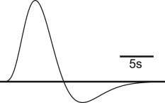
Canonical HRF used to generate the artificial time courses.
There were thus 3 locations, 3 numbers of spikes per run, and 11 HRF amplitudes (7 fixed and 4 randomly varying) for a total of 99 possible combinations of parameters. For each of the five patients, all combinations were used with five randomly determined spike timings, yielding 2,475 simulated datasets. Examples of artificial time courses are shown in Figure 2.
Figure 2.
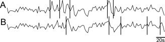
Simulated BOLD responses to epileptic spikes superimposed on background fMRI data. Vertical bars indicate random spike timings. (A) With a simulated HRF amplitude of 2% of the mean background fMRI signal value, the HRF peaks are clearly visible following the spikes. (B) Same background fMRI data, with different spike timings and HRF amplitude of only 0.5% of the mean fMRI signal value.
To evaluate the robustness of traditional analysis methods based on the GLM when the HRF is mis‐specified, an additional dataset was created using a noncanonical HRF formed by a single gamma function peaking 3 s later than the canonical shape and without undershoot. This dataset used 5 spikes per scanning run and a constant HRF amplitude of 1% of the mean fMRI signal value. For each patient, these time courses were superimposed on the same three cortical regions determined previously.
Data Preprocessing
The simulated data were first corrected for timing differences between the acquisitions of each slice. This was accomplished by resampling the fMRI time courses to the acquisition time of the top slice using sinc interpolation with Hanning windowing to attenuate ringing artifacts. Scanner drift was removed by high‐pass filtering. For each patient, all scanning runs were then concatenated. A method based on ICA was then applied on the data to try to recover the simulated activation regions. The method is summarized in Figure 3 and described in detail in the following sections.
Figure 3.
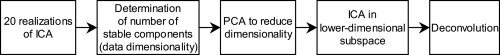
Schematic representation of the data processing steps. Twenty ICA decompositions are applied to the preprocessed data, and the number of reproducible components is determined. An additional ICA is then performed in the lower‐dimensional subspace extracted by PCA, and whose dimension is determined by the number of stable components. A deconvolution method is then applied to identify components related to the simulated spikes.
Independent Component Analysis
ICA assumes that the fMRI data can be represented as a linear mixture of spatially independent sources
where X is the matrix of observed fMRI images at each time frame, S is the matrix of independent sources, A is the linear mixing matrix representing the contribution of the sources at each time point, and η is a matrix of additive Gaussian noise.
ICA consists of estimating the sources and the mixing matrix, given only the observed mixtures. One possible approach is to use iterative optimization methods to obtain maximally non‐Gaussian sources, which is equivalent to maximizing statistical independence [Hyvarinen and Oja,2000]. It can be shown that the independent non‐Gaussian components are uniquely identifiable, if the number of sources is known a priori or can be reliably estimated [Beckmann and Smith,2004]. In this case, principal component analysis (PCA) can be used to first reduce the data into a principal subspace of dimensionality equal to the number of sources to extract. Decomposition within a higher‐dimensional subspace could result in sources being split into several components. Methods based on the application of information‐theoretic criteria to the eigenspectrum can provide a good estimate of the dimensionality of the data, but only if the covariance of the noise is known [Cordes and Nandy,2006]. Otherwise, the estimated number of sources tends to be proportional to the number of time points in the fMRI acquisition, an unrealistic assumption.
It was decided instead to use a criterion of reproducibility to determine the number of components to extract. In many ICA algorithms, the mixing matrix is initialized with random values and iteratively optimized to maximize the independence between the sources. This stochastic aspect results in a potentially different decomposition for each application of ICA on the same data. Nevertheless, components representing true independent sources are more likely to appear consistently across ICA realizations [Himberg et al.,2004]. Therefore, ICA was applied several times on the preprocessed fMRI data to determine how many components occurred consistently in each realization. It would then be possible to consider those reproducible components as the true sources composing the data. However, since ICA has been applied on the original high‐dimensional data, the sources may actually have been split into multiple components. It was thus decided to use only the number of reproducible components as an estimate of the dimensionality of the data. This estimate is then used to reduce the dimensionality of the original dataset using PCA. An additional application of ICA on this dimensionality‐reduced dataset was then used to obtain the final decomposition of the data.
In detail, for each patient, 20 repetitions of probabilistic ICA [Beckmann and Smith,2004], as implemented in FSL software [Smith et al.,2004], were applied on the fMRI data with a random initial seed. As the order of the components extracted by ICA is stochastic, it was then necessary to identify, in all ICA decompositions, the components corresponding to the same source. Cross‐correlation coefficients were computed between each spatial map and all the maps from other realizations. Highly cross‐correlated components were then clustered following the methods of Yang et al. [2008]. Specifically, the pair of spatial maps with maximum absolute correlation coefficient is first identified. Spatial maps in the remaining 18 ICA decompositions not yet belonging to the cluster with maximum correlation coefficient with either of the spatial maps in the first pair are then added to the cluster. The cluster is thus complete when it contains exactly one spatial map from each of the 20 ICA realizations. The procedure is repeated to determine the next cluster of components, finding the maximum correlation coefficient among the remaining spatial maps. A reproducibility index is then calculated by summing the absolute correlation coefficients between all pairs of spatial maps belonging to each cluster. Since there are 20 spatial maps in each cluster, the maximum value of the reproducibility index is  . Clusters with a reproducibility index above 50% of this maximum value were considered to represent stable components, as recommended by Yang et al.,2008. As described above, PCA was then used to project the data onto its principal subspace of dimension equal to the number of stable components. The sources making up the data were then extracted by an additional application of ICA within this subspace of lower dimensionality. It was then necessary to identify which components represented the simulated epileptic activity. A deconvolution method [Lu et al.,2006,2007] was applied to detect time courses that showed significant changes following the spike timings, without constraining the HRF to a canonical shape. This method uses a basis set formed by separate regressors modeling the amplitude of the HRF for each time lag following the spikes, up to the maximum expected length of the response. The amplitude of each regressor is allowed to vary freely; the basis set can thus represent HRFs of arbitrary shapes. It was decided to use a basis set representing the HRF amplitude at intervals of 1 s following the spikes, with a maximum HRF duration of 32 s [Lu et al.,2006]. Since the fMRI data were only acquired with a TR of 3 s, they were upsampled using linear interpolation to obtain a signal value every second.
The basis set convolved with the spike timings was then fitted to the ICA time courses in the GLM framework using ordinary least squares (OLS). This approach only assumes that each spike is followed by a consistent HRF, regardless of its shape. Components not related to the spikes should yield HRFs that are indistinguishable from the background noise. Statistical significance was determined using an F‐test on the fitted HRF. Although OLS assumes that the noise is temporally uncorrelated, this was not the case due to the upsampling of the ICA time course and the autocorrelations that are known to exist in fMRI data [Friston et al.,2000]. The noise was modeled as an autoregressive (AR) process estimated from the OLS residuals. Specifically, the Yule–Walker equations were used to estimate the partial autocorrelation coefficients from the sample autocorrelation of the residuals. The order of the AR process was determined by performing the estimation with gradually increasing AR orders, until the highest‐order coefficient was no longer statistically significant (P < 0.05). These parameters were then used to perform an adjusted F‐test with an appropriately weighted F‐statistic and effective degrees of freedom [Kruggel et al.,2002].
The adjusted F‐tests were used to detect components with a fitted HRF accounting for a statistically significant portion of the time course variance (P < 0.05, Bonferroni‐corrected for the number of components being examined). A Gaussian and two Gamma distributions, representing background noise, activations, and deactivations, were used in a mixture model to fit the distributions of voxel intensities in the spatial maps of the identified components [Beckmann and Smith,2004]. These maps were then thresholded to identify voxels with a probability of activation or deactivation greater than 99.9%. The activated or deactivated voxels could then be compared with the known activation regions used in the simulated datasets.
Since the ICA and deconvolution methods are independent of the shape of the HRF, it was expected that the performance would be identical whether the simulated data were generated with a canonical or a noncanonical HRF. On the other hand, analysis using the GLM is critically dependent on the appropriate representation of the HRF. In addition to ICA, the dataset generated with the noncanonical HRF was also analyzed using the GLM [Worsley et al.,2002]. Statistical t‐maps were generated assuming a canonical HRF to the simulated spikes for each voxel. The maps were then thresholded at |t| > 3.1 (corresponding to P < 0.001, uncorrected). A spatial extent threshold of 3 voxels was then applied to achieve a corrected cluster P‐value of 0.05 [Friston et al.,1994]. It was then possible to evaluate the performance of the GLM method when applied to data that deviated slightly from the assumption of a canonical HRF.
RESULTS
The number of reproducible components in the multiple ICA decompositions ranged from 222 to 353. The number of components was highly correlated with the number of scanning runs used for each patient (Pearson's r = 0.98, P < 0.01).
In 2,089 out of 2,475 simulations (84.4%), a significant component was detected with spatial topography consisting of one activated cluster accounting for at least 10 voxels in the simulated region. In the following, these components will be referred as “concordant components”; an example of activation map is shown in Figure 4, where the fitted HRF resembles closely the canonical HRF. In 37.2% of these components, the activated cluster was actually slightly larger than the simulated region, containing at least 1 voxel immediately adjacent to this region. 7.0% of the concordant components contained a single isolated activated voxel at another location, while 4.9% had more than one false positive voxel. These falsely activated voxels were generally isolated at locations without any recognizable pattern. Figure 5 shows time courses from a simulation, which resulted in a falsely activated voxel that coincidentally occurred in the same slice as a 3 × 3 region of voxels corresponding to the simulated active region. The figure shows an excerpt of the time courses of the falsely activated voxel, of the central voxel of the activated region, of the simulated spike‐related signal, and of the concordant ICA component. The time course of the voxel in the true activated region is shown prior to superimposing on it the simulated signal. There is a small but significant correlation (r = 0.13, P < 0.01) between that time course and that of the falsely activated voxel. The average correlation between the falsely activated voxel and the 27 voxels comprising the active region was 0.19, with 24 of the correlations being significant (P < 0.05, Bonferroni‐corrected). After superimposing the low‐amplitude simulated spike‐related signal (HRF of 1.25% of the mean fMRI signal) in the activated region, the average correlation was 0.18, with the same 24 voxels still showing significant correlation (P < 0.05, Bonferroni‐corrected). It is not clear whether the significant correlations between the falsely activated voxel and the activated region are due to actual functional connectivity between these regions. Nevertheless, it is not surprising that ICA groups these two regions in a single component. Adjacent voxels are more likely to be functionally connected; hence the relatively large proportion of simulations with falsely activated voxels immediately adjacent to the truly active region (although not in the example of Fig. 5).
Figure 4.
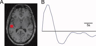
(A) Activation map corresponding exactly to the simulated activation region in the displayed plane. (B) Significant HRF fitted by the deconvolution method, matching the original simulated canonical HRF.
Figure 5.
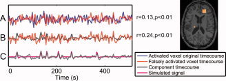
Time courses of a simulation yielding a concordant component (3 × 3 activated right frontal region shown in the spatial map) and a falsely activated voxel (left posterior). (A) The time courses of the falsely activated voxel and of the central voxel of the activated region, prior to superimposing the simulated spike‐related signal, are significantly correlated (r = 0.13, P < 0.01). (B) The time course of the concordant component is significantly correlated (r = 0.24, P < 0.01) with the time course of the falsely activated voxel. (C) Component time course and simulated spike‐related signal.
In addition, 303 simulations (12.2%) resulted in the identification of a component with a time course that was significantly related to the spike timings, but with spatial topography that did not correspond to the simulated activation region (in 96.7% of cases, there were no activated voxels in the simulated region; the remaining 3.3% had fewer than 10 true positive voxels). Henceforth, these components will be referred as “discordant components.” Typically, the erroneous activations consisted of clusters near brain boundaries or in the ventricles. An example of such a component is shown in Figure 6. This spatial pattern is typical of residual motion artifact that may persist even after motion correction. Moreover, the time course of this discordant component shows sudden sharp transients that seem to match the z‐direction translation parameters determined during motion correction. The movements occurred shortly following three of the random simulated spikes. Even though it is improbable that movement would follow every spike, the residual artifact may still be large enough for the deconvolution method to determine that the component is significantly related to the spike timings. A single high‐amplitude movement‐related transient following only one of the simulated spikes may be sufficient to be falsely detected by the method, as it causes a violation of the assumption of stationarity of the residuals in the GLM used for the deconvolution.
Figure 6.
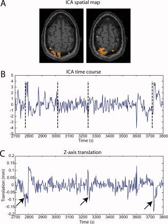
(A) Two slices of a typical spatial map of a significant component that was not concordant with the simulated activation region. The activation cluster at the edge of the brain suggests a residual motion artifact. (B) Part of the time course of the same component, with vertical dashed bars showing the timings of the simulated spikes. Sharp transients follow some of the spike timings. (C) Translation in the z‐direction determined from the motion correction preprocessing step. The arrows show that the transients found in panel B seem to correspond to residual motion artifacts. [Color figure can be viewed in the online issue, which is available at www.interscience.wiley.com.]
Simulations With Constant HRF Amplitude
Figure 7 summarizes the percentage of simulations where concordant components could be detected for different levels of constant HRF amplitudes, the proportion of simulations yielding discordant components, and the average number of falsely activated voxels found in concordant components.
Figure 7.
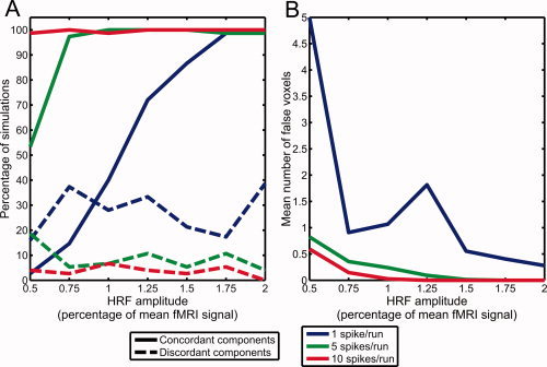
(A) Percentage of simulations with constant HRF amplitudes where significant components were found, either correctly matching the simulated activation region (concordant components) or at another location (discordant components). (B) Mean number of falsely activated voxels in concordant components.
In simulations with 10 spikes per run and constant HRF amplitude, concordant components could almost always be found, with a sensitivity greater than 97% for all tested HRF amplitudes. However, HRF amplitudes of at least 0.75% of the mean fMRI signal with 5 spikes per run, or 1.75% with 1 spike per run, were necessary to reach the same 97% sensitivity. The sensitivity was greatly reduced at lower HRF amplitudes. For example, the sensitivity was only 53.3% with 0.5% HRF amplitude and 5 spikes per run, and the sensitivity was below 50% for HRF amplitudes of 1% or less and 1 spike per run. The average number of falsely activated voxels was highest for simulations with 1 spike per run and 0.5% HRF amplitude, where the low variance of the simulated signal does not greatly affect the correlations already present in the background fMRI data.
Discordant components were detected in only 3.6% of the simulations with 10 spikes per run, 8.8% of simulations with 5 spikes per run, and 26.7% of simulations with 1 spike per run.
Large movement artifacts occurring at the same time as the spikes may be fitted by the deconvolution method. In simulations with a low number of spikes, these artifacts are more likely to account for a significant amount of variance in relation to the simulated BOLD responses to the spikes. Hence these artifactual components tend to show as discordant components in simulations with only 1 spike per run, resulting in a higher percentage of simulations with discordant components.
Simulations With Varying HRF Amplitude
Similar results were obtained when the HRF amplitude varied randomly (see Fig. 8). In simulations with 10 spikes per run or 5 spikes per run, a concordant component was detected in more than 99% of the cases. However, when there was only 1 spike per run, a concordant component could only be identified in 57.3% of the cases. When only considering simulations with a mean HRF amplitude of at least 1.25%, the proportion of cases resulting in the identification of a concordant component increased to 84.0%.
Figure 8.
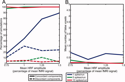
(A) Percentage of simulations with varying HRF amplitudes where significant components were found, either correctly matching the simulated activation region (concordant components) or at another location (discordant components). (B) Mean number of falsely activated voxels in concordant components.
As for discordant components, they occurred in 4.0% of simulations with 10 spikes per run, 5.3% of simulations with 5 spikes per run, and 22.0% of simulations with 1 spike per run. Similar to the simulations with constant HRF amplitude, the spatial maps corresponding to the discordant components often included voxels near brain boundaries, suggesting that they represented residual movement artifacts.
Simulations With Noncanonical HRF
The noncanonical HRF used in these simulations was significantly correlated with the standard canonical HRF (Pearson's r = 0.26, P < 0.001). In 14 of the 15 datasets generated with this noncanonical HRF, the ICA method successfully extracted a concordant component. No discordant components were erroneously detected. However, analysis using the GLM, assuming a canonical HRF, could only find a significant cluster at the correct location in 3 of 15 datasets. The sizes of these clusters were 5, 5, and 11 voxels, respectively, which is smaller than the original simulated activation region of size 27 voxels. One of these three datasets also had a significant cluster at another location in the brain outside of the simulated activation region. Such a false activation was also found in 2 of the 12 datasets that did not have a significant cluster in the correct location. The remaining 10 t‐maps did not contain any significant clusters.
DISCUSSION
Simulation Parameters
The results reveal the conditions under which the ICA method could detect the simulated activations. The range of HRF amplitudes from 0.5 to 2% corresponded to typical values in realistic fMRI data [Gu et al.,2001]. Studies investigating the BOLD response to epileptic spikes have found large variations in amplitude across patients and brain regions [Benar et al.,2002; Gotman et al.,2006]. HRF amplitudes as high as 5% or less than 0.5% of the baseline fMRI signal were reported. However, a HRF amplitude of 2% was sufficient to detect the simulated activations in almost all test cases, so larger amplitudes were not examined. At low amplitudes, the BOLD signal change can be very difficult to detect, as it is smaller than background noise levels. ICA separates structured noise components [Perlbarg et al.,2007; Thomas et al.,2002], allowing the detection of small amplitude activations.
The number of spikes per 6‐min scanning run also greatly influenced the ability of the method to detect the simulated activations. Patients undergoing EEG‐fMRI studies are usually selected on the basis of having frequent epileptic discharges visible on the EEG [Krakow et al.,1999; Laufs and Duncan,2007]. There is a tendency to detect significant responses more frequently with higher spiking rates [Al Asmi et al.,2003]. However, activations may sometimes be detected with only a few spikes, and having a large number of spikes does not guarantee that a significant response will be found. Studies with high spiking rates (more than 2 or 3 per minute) have revealed nonlinear effects of the HRF due to the saturation of the overlapping BOLD responses to closely spaced events [Jacobs et al.,2008; Salek‐Haddadi et al.,2006]. These high spiking rates are greater than the maximal rate of 10 spikes per run used in the simulations. Although the artificial time courses were generated in a way that preserved the linearity of the response, it should be noted that ICA does not depend on a linear assumption to detect spatial patterns related to the spikes. However, the identification of the relevant component using the deconvolution method does assume that there is a consistent linear response.
The simulated activation size of 3 × 3 × 3 voxels (5‐mm isotropic resolution) corresponds to a volume of 3.375 cm3, which is a typical size for fMRI spike‐related activation. Early experiments have suggested that spikes visible on scalp EEG were the result of an active synchronized cortical area of at least 6 cm2 [Cooper et al.,1965], although figures ranging from 10 to 20 cm2 have been proposed more recently [Tao et al.,2007]. In terms of volume, EEG‐fMRI studies have yielded similar volumes of activation, such as an average of 3.3 cm3 reported by [Lemieux et al.,2001] or an average of 3.06 cm3 found by [Al Asmi et al.,2003]. It should be noted that the fMRI activation volume is often closely linked to the statistical threshold used. Nevertheless, in the absence of any gold standard to accurately determine the volume of activation, the region size for the simulation was an appropriate realistic choice.
Although simulations cannot reproduce all the conditions present in real data, they still provide a controlled way of evaluating the performance of the ICA method under realistic parameters. The proposed method could clearly identify a spatial map that corresponded to the simulated region of activation unless the number of spikes or HRF amplitude were smaller than the expected range of values found in real data.
Component Identification
The application of ICA to fMRI relies on the assumption that ICA can provide a good separation of the data into its constituent sources. However, the results may depend on the number of components selected for the decomposition. Currently, there is no consensus on the most appropriate way of determining the dimensionality of the fMRI dataset, and several methods have been proposed [Beckmann and Smith,2004; Cordes and Nandy,2006; Li et al.,2007; Yang et al.,2008]. Nevertheless, identifying reproducible components in multiple ICA decompositions at least eliminates noisy components due to the stochastic nature of the algorithm. Moreover, the additional application of ICA on a subspace of reduced dimensionality helps reduce the degradation that occurs when overfitting the ICA model with too many components in the original decompositions [Li et al.,2007]. It should also be noted that the dimensionality used for the final application of ICA was higher than some values reported in the literature [Cordes and Nandy,2006; Li et al.,2007; Rodionov et al.,2007], which were less than 100, although we had larger datasets. Extracting a large number of components may prevent relevant signals of very low amplitude from being missed by the decomposition. It is hoped that the development of better dimensionality estimation results in better decompositions in the future. Nevertheless, it should be noted that our empirical results suggest that the method used can extract valid spike‐related components in simulations with realistic signal amplitude.
Data‐driven methods such as ICA can identify common spatial patterns in the fMRI signal without the need for a priori assumptions about the location of the activation or the timing of the epileptic activity. Other methods such as TCA [Morgan et al.,2004] also have shown the potential to reveal hemodynamic correlates of epileptic activity based purely on the analysis of the BOLD signal. However, it then becomes a problem to validate the extracted patterns of activation and determine if they truly represent epileptic activity. The use of concurrently recorded EEG thus seems to be necessary to identify brain areas that show BOLD changes in response to epileptic spikes [Hamandi et al.,2005]. The nature of these BOLD changes is still not clearly defined, and the variability in the shape of the HRF may affect the results of purely hypothesis‐driven methods. On the other hand, ICA can detect components representing epileptic activity regardless of the shape of the BOLD response. The spike timings provided by EEG are only used in a posterior analysis to identify the appropriate components.
In another study using ICA on fMRI data acquired during a sensorimotor task, the component selection was performed using a priori knowledge of the expected spatial topography of the task, namely the auditory and sensorimotor cortices [Gu et al.,2001]. However, in epilepsy patients, the region of activation cannot be known in advance, and it is expected that EEG‐fMRI could provide localization information to complement other modalities. This precludes the use of precise spatial priors for ICA components identification. It would be possible to convolve the spike timings with a canonical HRF, finding component time courses highly correlated with this model. However, this method would not identify BOLD responses with an HRF that is substantially different from the canonical shape. The deconvolution method is seen as a good compromise between hypothesis‐driven and data‐driven methods. It does not restrict the shape of the HRF, and only assumes that the HRF is linear and consistent for each spike. Nevertheless, it would be interesting to develop a method that would take into account possible nonlinear effects. As for the consistency of the HRF, some variability has been reported, even in adjacent brain regions [Gotman et al.,2006]. The robustness of the method was thus evaluated by generating time courses with randomly varying HRF amplitude. Components with spatial topography matching the simulated activation region could still be found when there were a sufficient number of spikes or large enough mean HRF amplitude. Compared to the simulations with constant HRF amplitudes, the performance of the method, given the same mean HRF amplitude, was only slightly degraded for simulations with random amplitudes.
The deconvolution method would be particularly effective if the HRF had a consistent shape, even similar to the canonical shape, but with an unknown time‐to‐peak. The simulations showed that the performance of the GLM analysis, assuming a canonical HRF, could be greatly affected in this case. Variations from the canonical delay of the HRF to epileptic spikes have been reported, such as for negative BOLD responses, which tend to occur later than positive responses [Bagshaw et al.,2004]. BOLD changes occur before the spikes have even been found, perhaps due to electrical activity that did not result in visible discharges on the scalp [Hawco et al.,2007]. A study using ICA on EEG‐fMRI data found component time courses that were maximally correlated with a canonical HRF model at a wide variety of lags [Rodionov et al.,2007]. The use of correlation with the GLM regressor might however prevent the identification of BOLD activations related to the spikes, but with an HRF different from the canonical shape. This study used an automated component classification scheme [De Martino et al.,2007] to reject components due to fMRI artifacts. The remaining components were then considered to represent BOLD responses to cerebral activity. However, a visual inspection was still necessary to distinguish components of epileptic activity from other unrelated brain processes and resting‐state networks. Nevertheless, the automated classification method could be used to eliminate many of the discordant components that were due to movements at the same time as the simulated spikes. A combination of the deconvolution method with this artifact rejection would thus be an effective way of automatically identifiying ICA components related to the spikes, without any constraints on the shape of the HRF.
CONCLUSION
Even though the artificial time courses were created with a canonical HRF, the method is independent of the HRF shape. ICA could provide a model‐free approach, robust to uncertainty and variability in the HRF, for the detection of activation regions in EEG‐fMRI data.
REFERENCES
- Aghakhani Y,Kobayashi E,Bagshaw A,Hawco C,Benar C,Dubeau F,Gotman J ( 2006): Cortical and thalamic fMRI responses in partial epilepsy with focal and bilateral synchronous spikes. Clin Neurophysiol 117: 177–191. [DOI] [PubMed] [Google Scholar]
- Aguirre G,Zarahn E,D'Esposito M ( 1998): The variability of human, BOLD hemodynamic responses. Neuroimage 8: 360–369. [DOI] [PubMed] [Google Scholar]
- Al Asmi A,Benar C,Gross D,Khani Y,Andermann F,Pike B,Dubeau F,Gotman J ( 2003): fMRI activation in continuous and spike‐triggered EEG‐fMRI studies of epileptic spikes. Epilepsia 44: 1328–1339. [DOI] [PubMed] [Google Scholar]
- Bagshaw A,Aghakhani Y,Benar C,Kobayashi E,Hawco C,Dubeau F,Pike G,Gotman J ( 2004): EEG‐fMRI of focal epileptic spikes: Analysis with multiple haemodynamic functions and comparison with gadolinium‐enhanced MR angiograms. Hum Brain Mapp 22: 179–192. [DOI] [PMC free article] [PubMed] [Google Scholar]
- Beckmann C,Smith S ( 2004): Probabilistic independent component analysis for functional magnetic resonance imaging. IEEE Trans Med Imaging 23: 137–152. [DOI] [PubMed] [Google Scholar]
- Benar C,Gross D,Wang Y,Petre V,Pike B,Dubeau F,Gotman J ( 2002): The BOLD response to interictal epileptiform discharges. Neuroimage 17: 1182–1192. [DOI] [PubMed] [Google Scholar]
- Benar C,Aghakhani Y,Wang Y,Izenberg A,Al Asmi A,Dubeau F,Gotman J ( 2003): Quality of EEG in simultaneous EEG‐fMRI for epilepsy. Clin Neurophysiol 114: 569–580. [DOI] [PubMed] [Google Scholar]
- Cooper R,Winter A,Crow H,Walter W ( 1965): Comparison of subcortical, cortical and scalp activity using chronically indwelling electrodes in man. Electroencephalogr Clin Neurophysiol 18: 217–228. [DOI] [PubMed] [Google Scholar]
- Cordes D,Nandy R ( 2006): Estimation of the intrinsic dimensionality of fMRI data. Neuroimage 29: 145–154. [DOI] [PubMed] [Google Scholar]
- De Martino F,Gentile F,Esposito F,Balsi M,Di Salle F,Goebel R,Formisano E ( 2007): Classification of fMRI independent components using IC‐fingerprints and support vector machine classifiers. Neuroimage 34: 177–194. [DOI] [PubMed] [Google Scholar]
- Federico P,Archer J,Abbott D,Jackson G ( 2005): Cortical/subcortical BOLD changes associated with epileptic discharges: An EEG‐fMRI study at 3 T. Neurology 64: 1125–1130. [DOI] [PubMed] [Google Scholar]
- Friston K,Worsley K,Frackowiak R,Mazziotta J,Evans A ( 1994): Assessing the significance of focal activations using their spatial extent. Hum Brain Mapp 1: 210–220. [DOI] [PubMed] [Google Scholar]
- Friston K,Josephs O,Rees G,Turner R ( 1998): Nonlinear event‐related responses in fMRI. Magn Reson Med 39: 41–52. [DOI] [PubMed] [Google Scholar]
- Friston K,Josephs O,Zarahn E,Holmes A,Rouquette S,Poline J ( 2000): To smooth or not to smooth? Bias and efficiency in fMRI time‐series analysis. Neuroimage 12: 196–208. [DOI] [PubMed] [Google Scholar]
- Glover G ( 1999): Deconvolution of impulse response in event‐related BOLD fMRI. Neuroimage 9: 416–429. [DOI] [PubMed] [Google Scholar]
- Gotman J,Kobayashi E,Bagshaw A,Benar C,Dubeau F ( 2006): Combining EEG and fMRI: A multimodal tool for epilepsy research. J Magn Reson Imaging 23: 906–920. [DOI] [PubMed] [Google Scholar]
- Gu H,Engelien W,Feng H,Silbersweig D,Stern E,Yang Y ( 2001): Mapping transient, randomly occurring neuropsychological events using independent component analysis. Neuroimage 14: 1432–1443. [DOI] [PubMed] [Google Scholar]
- Hamandi K,Salek‐Haddadi A,Liston A,Laufs H,Fish D,Lemieux L ( 2005): fMRI temporal clustering analysis in patients with frequent interictal epileptiform discharges: Comparison with EEG‐driven analysis. Neuroimage 26: 309–316. [DOI] [PubMed] [Google Scholar]
- Handwerker D,Ollinger J,D'Esposito M ( 2004): Variation of BOLD hemodynamic responses across subjects and brain regions and their effects on statistical analyses. Neuroimage 21: 1639–1651. [DOI] [PubMed] [Google Scholar]
- Hawco C,Bagshaw A,Lu Y,Dubeau F,Gotman J ( 2007): BOLD changes occur prior to epileptic spikes seen on scalp EEG. Neuroimage 35: 1450–1458. [DOI] [PubMed] [Google Scholar]
- Himberg J,Hyvarinen A,Esposito F ( 2004): Validating the independent components of neuroimaging time series via clustering and visualization. Neuroimage 22: 1214–1222. [DOI] [PubMed] [Google Scholar]
- Hyvarinen A,Oja E ( 2000): Independent component analysis: Algorithms and applications. Neural Netw 13: 411–430. [DOI] [PubMed] [Google Scholar]
- Jacobs J,Hawco C,Kobayashi E,Boor R,Levan P,Stephani U,Siniatchkin M,Gotman J ( 2008): Variability of the hemodynamic response as a function of age and frequency of epileptic discharge in children with epilepsy. Neuroimage 40: 601–614. [DOI] [PMC free article] [PubMed] [Google Scholar]
- Krakow K,Woermann F,Symms M,Allen P,Lemieux L,Barker G,Duncan J,Fish D ( 1999): EEG‐triggered functional MRI of interictal epileptiform activity in patients with partial seizures. Brain 122(Part 9): 1679–1688. [DOI] [PubMed] [Google Scholar]
- Kruggel F,Pelegrini‐Issac M,Benali H ( 2002): Estimating the effective degrees of freedom in univariate multiple regression analysis. Med Image Anal 6: 63–75. [DOI] [PubMed] [Google Scholar]
- Laufs H,Duncan J ( 2007): Electroencephalography/functional MRI in human epilepsy: What it currently can and cannot do. Curr Opin Neurol 20: 417–423. [DOI] [PubMed] [Google Scholar]
- Lemieux L,Krakow K,Fish D ( 2001): Comparison of spike‐triggered functional MRI BOLD activation and EEG dipole model localization. Neuroimage 14: 1097–1104. [DOI] [PubMed] [Google Scholar]
- Lemieux L,Laufs H,Carmichael D,Paul J,Walker M,Duncan J ( 2008): Noncanonical spike‐related BOLD responses in focal epilepsy. Hum Brain Mapp 29: 329–345. [DOI] [PMC free article] [PubMed] [Google Scholar]
- Li Y,Adali T,Calhoun V ( 2007): Estimating the number of independent components for functional magnetic resonance imaging data. Hum Brain Mapp 28: 1251–1266. [DOI] [PMC free article] [PubMed] [Google Scholar]
- Lu Y,Bagshaw A,Grova C,Kobayashi E,Dubeau F,Gotman J ( 2006): Using voxel‐specific hemodynamic response function in EEG‐fMRI data analysis. Neuroimage 32: 238–247. [DOI] [PubMed] [Google Scholar]
- Lu Y,Grova C,Kobayashi E,Dubeau F,Gotman J ( 2007): Using voxel‐specific hemodynamic response function in EEG‐fMRI data analysis: An estimation and detection model. Neuroimage 34: 195–203. [DOI] [PubMed] [Google Scholar]
- McKeown M,Makeig S,Brown G,Jung T,Kindermann S,Bell A,Sejnowski T ( 1998): Analysis of fMRI data by blind separation into independent spatial components. Hum Brain Mapp 6: 160–188. [DOI] [PMC free article] [PubMed] [Google Scholar]
- Menz M,Neumann J,Muller K,Zysset S ( 2006): Variability of the BOLD response over time: An examination of within‐session differences. Neuroimage 32: 1185–1194. [DOI] [PubMed] [Google Scholar]
- Morgan V,Price R,Arain A,Modur P,Abou‐Khalil B ( 2004): Resting functional MRI with temporal clustering analysis for localization of epileptic activity without EEG. Neuroimage 21: 473–481. [DOI] [PubMed] [Google Scholar]
- Perlbarg V,Bellec P,Anton J,Pelegrini‐Issac M,Doyon J,Benali H ( 2007): CORSICA: Correction of structured noise in fMRI by automatic identification of ICA components. Magn Reson Imaging 25: 35–46. [DOI] [PubMed] [Google Scholar]
- Rodionov R,De Martino F,Laufs H,Carmichael D,Formisano E,Walker M,Duncan J,Lemieux L ( 2007): Independent component analysis of interictal fMRI in focal epilepsy: Comparison with general linear model‐based EEG‐correlated fMRI. Neuroimage 38: 488–500. [DOI] [PubMed] [Google Scholar]
- Salek‐Haddadi A,Diehl B,Hamandi K,Merschhemke M,Liston A,Friston K,Duncan J,Fish D,Lemieux L ( 2006): Hemodynamic correlates of epileptiform discharges: An EEG‐fMRI study of 63 patients with focal epilepsy. Brain Res 1088: 148–166. [DOI] [PubMed] [Google Scholar]
- Smith S,Jenkinson M,Woolrich M,Beckmann C,Behrens T,Johansen‐Berg H,Bannister P,De Luca M,Drobnjak I,Flitney D,Niazy R,Saunders J,Vickers J,Zhang Y,De Stefano N,Brady J,Matthews P ( 2004): Advances in functional and structural MR image analysis and implementation as FSL. Neuroimage 23( Suppl 1): S208–S219. [DOI] [PubMed] [Google Scholar]
- Srivastava G,Crottaz‐Herbette S,Lau K,Glover G,Menon V ( 2005): ICA‐based procedures for removing ballistocardiogram artifacts from EEG data acquired in the MRI scanner. Neuroimage 24: 50–60. [DOI] [PubMed] [Google Scholar]
- Tao J,Baldwin M,Hawes‐Ebersole S,Ebersole J ( 2007): Cortical substrates of scalp EEG epileptiform discharges. J Clin Neurophysiol 24: 96–100. [DOI] [PubMed] [Google Scholar]
- Thomas C,Harshman R,Menon R ( 2002): Noise reduction in BOLD‐based fMRI using component analysis. Neuroimage 17: 1521–1537. [DOI] [PubMed] [Google Scholar]
- Worsley K,Friston K ( 1995): Analysis of fMRI time‐series revisited—Again. Neuroimage 2: 173–181. [DOI] [PubMed] [Google Scholar]
- Worsley K,Liao C,Aston J,Petre V,Duncan G,Morales F,Evans A ( 2002): A general statistical analysis for fMRI data. Neuroimage 15: 1–15. [DOI] [PubMed] [Google Scholar]
- Yang Z,Laconte S,Weng X,Hu X ( 2008): Ranking and averaging independent component analysis by reproducibility (RAICAR). Hum Brain Mapp 29: 711–725. [DOI] [PMC free article] [PubMed] [Google Scholar]