

Abstract
Inference of haplotypes is important for many genetic approaches, including the process of assigning a phenotype to a genetic region. Usually, the population frequencies of haplotypes, as well as the diplotype configuration of each subject, are estimated from a set of genotypes of the subjects in a sample from the population. We have developed an algorithm to infer haplotype frequencies and the combination of haplotype copies in each pool by using pooled DNA data. The input data are the genotypes in pooled DNA samples, each of which contains the quantitative genotype data from one to six subjects. The algorithm infers by the maximum-likelihood method both frequencies of the haplotypes in the population and the combination of haplotype copies in each pool by an expectation-maximization algorithm. The algorithm was implemented in the computer program LDPooled. We also used the bootstrap method to calculate the standard errors of the estimated haplotype frequencies. Using this program, we analyzed the published genotype data for the SAA (n=156), MTHFR (n=80), and NAT2 (n=116) genes, as well as the smoothelin gene (n=102). Our study has shown that the frequencies of major (frequency >0.1 in a population) haplotypes can be inferred rather accurately from the pooled DNA data by the maximum-likelihood method, although with some limitations. The estimated D and D′ values had large variations except when |D| values were >0.1. The estimated linkage-disequilibrium measure ρ2 for 36 linked loci of the smoothelin gene when one- and two-subject pool protocols were used suggested that the gross pattern of the distribution of the measure can be reproduced using the two-subject pool data.
Introduction
Inference of haplotypes is important for many genetic approaches, including the process of assigning a phenotype to a genetic region (Risch et al. 1996; Hodge et al. 1999; Rieder et al. 1999). Extended marker haplotypes may provide additional power in the detection of associations (Kruglyak 1999; Templeton 1999; Judson et al. 2000; Martin et al. 2000; Zöllner and von Haeseler 2000).
In testing for the presence of linkage disequilibrium or in estimating its strength, the frequencies of haplotypes and the frequencies of alleles in a population should be evaluated. Thus, estimation of the haplotype frequencies in a population is the first step in analysis of linkage disequilibrium. On the one hand, when the family data are available, we can extract the phase data and either estimate or determine the haplotypes by using software such as Linkage Package (Lathrop et al. 1985) and Genehunter (Kruglyak et al. 1996). On the other hand, when the family data are not available, Hardy-Weinberg equilibrium is assumed for the population data, and the haplotype frequencies are estimated by the parsimony method (Clark 1990), the expectation-maximization (EM) algorithm (Excoffier and Slatkin 1995; Hawley and Kidd 1995; Long et al. 1995; Kitamura et al. 2002), or the Phase algorithm, which is based on Bayesian inference (Stephens et al. 2001). Fallin and Schork (2000) have demonstrated high accuracy in haplotype-frequency estimation for biallelic diploid samples by use of the EM algorithm. We previously developed a program, LDSupport, that estimates both haplotype frequencies in a population and the diplotype configuration for each subject (Kitamura et al. 2002). A diplotype configuration is a combination of two haplotype copies in a subject. Recently, Zhang et al. (2001) and Xu et al. (2002) compared Phase- and EM-algorithm–based methods and reported that the two methods exhibited similar performance, whereas Stephens et al. (2001) argued that the Phase method outperformed the EM method.
In the present study, we extended the function of LDSupport and constructed a new algorithm so that our program can handle genotype data from pooled DNA samples. Using published and unpublished data, we tested the accuracy of haplotype frequencies estimated by the new algorithm implemented in the new program, LDPooled.
Methods
DNA Pools
Suppose that we have genomic DNA samples from many subjects. Because of limitations of either cost or time, we wish to reduce the total number of typings. We therefore make N DNA pools, each of which contains the samples from M different subjects. The selection of the samples for pooling of DNA is performed at random, and the sample from a subject is selected only once. We then perform quantitative DNA typing by using each DNA pool for L linked loci. The loci can be either biallelic or multiallelic. The numbers of allele copies for each locus are assumed to be accurately determined by the quantitative DNA typing. By the terms “an allele copy” and “a haplotype copy,” we refer to an allele or a haplotype carried at a particular locus by a particular subject or a particular pool. If a subject is homozygous at a locus, then he or she is interpreted as carrying an allele but two allele copies at that locus. Note that there should be 2M allele copies (not 2M alleles) at a locus in a single pool and that, when M=1 (i.e., a single-subject pool), the situation is equivalent to general DNA typing for each subject.
EM Algorithm
Step 1: Assignment of real values to haplotype frequencies.—Let Ai be the number of alleles at the ith locus. The number of possible haplotypes for L loci is U=i=1LAi. We assign real values to the frequencies of haplotypes as the first step of the estimation. Let pi be the frequency of the ith haplotype in a population, where pi⩾0 for i=1,2,..,U. Naturally,  .
.
Step 2: Combination of haplotypes.—A pool of DNA contains samples from M subjects. Therefore, 2M haplotype copies should be present in a pool. When 2M haplotype copies are selected (permitting repetitive sampling) from the total of U haplotypes, at least one of the combinations of haplotype copies should be consistent with the observed pooled genotype data at all L loci for the pool. Let Cjm be the mth combination of haplotype copies that is consistent with the observed genotype data for the jth pool for L loci, where m=1,2,..,Qj. Qj denotes the number of combinations of haplotype copies consistent with the observed genotype data for the jth pool.
Step 3: Likelihood calculation.—Under the assumption of Hardy-Weinberg equilibrium, the prior probability of Cjm is
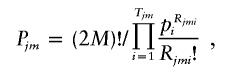 |
where Rjmi denotes the number of the copies of the ith haplotype within Cjm and Tjm denotes the number of different haplotypes within Cjm. Note that  for any j and m. The likelihood of the data for the jth pool given the haplotype frequencies is calculated as
  . Overall likelihood for all the N pools should be Lall=j=1NLj, since the events of combinations of haplotype copies for different subjects should be independent when Hardy-Weinberg equilibrium is assumed.
Step 4: Expectation.—The posterior probability of Cjm for the jth pool is calculated by Bayes’ theorem, as follows:
 |
Therefore, the expected number of copies of the ith haplotype in the entire pool is  .
.
Step 5: Maximization.—Maximization is performed by substituting Ei/(2MN) for pi for all i.
Step 6: Iteration.—Steps 2–5 are repeated until Lall converges. Lmax denotes the value of Lall when it converged. The value of pi after the final step of iteration is interpreted as  , the maximum-likelihood estimate of pi.
Calculation of Posterior Probability of Cjm Given the Maximum-Likelihood Estimates
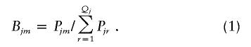
The posterior probability of Cjm for the jth pool, given that the population frequencies of the haplotypes are  for i=1,2,..,U, is obtained by applying the obtained estimates to steps 2–4. Thus, Bjm as obtained by equation (1) yields the posterior probability of Cjm for the jth pool, given that the population frequencies of the haplotypes are
  for i=1,2,..,U.
Likelihood under the Assumption of No Linkage Disequilibrium
Calculation of the likelihood of data under the assumption of no linkage disequilibrium was performed as follows: Let qik be the frequency of the kth allele at the ith locus in the population, let Vijk be the number of copies of the kth alleles at the ith locus in the jth pool, and let Wij be the number of different alleles at the ith locus in the jth pool. Note that  for any i and j. The likelihood of the data for the jth pool at the ith locus under the assumption of no linkage disequilibrium is
 |
Since alleles at different loci are independent under the assumption of no linkage disequilibrium, the likelihood of the data at all the loci should be i=1LSij, and the likelihood of the data at all the loci in all the pools should be Lindependent=j=1Ni=1LSij.
LOD Score
LOD score was calculated as follows:
 |
To exclude the null hypothesis of no linkage disequilibrium, we calculated the P value by incorporating the likelihood ratio in equation (2) as -ln (likelihood ratio) and assuming that this statistic asymptotically follows a χ2 distribution. The degrees of freedom should be
 |
Variation of Haplotype Frequencies, D, and D′ Determined by the Pooling Method
The estimated haplotype frequencies from the pooled genotype data exhibit variation due to different combinations of samples. To examine such variation, we made different combinations of the DNA samples from different subjects, to estimate haplotype frequencies. Thus, if there are a total of MN subjects and the samples from M different subjects should be in each pool, then N pools should be made. There are then  different combinations of the samples. This number is so large that we cannot examine all cases. We therefore used a Monte Carlo method to sample the combinations of N pools while assuming an equal probability for each of the combinations. From each sample, haplotype frequencies and pairwise linkage-disequilibrium measures D and D′ were estimated, as described below. From the estimates from 1,000 different randomly selected samples, means and SDs were calculated.
Nonparametric Bootstrap Method to Estimate SEs
The nonparametric bootstrap method was used to estimate empirically the SEs of the frequency of the ith haplotype—that is,  . The original pools of DNA consisted of N pools, each of which contained DNA from M subjects. A bootstrap sample was constructed by drawing a new set of N pools from the original N pools through the permission of duplicate sampling. The data in the new set of pools were then applied to the algorithm for the estimation of the frequencies of the haplotypes—that is, pi for i=1,2,..,U. Let
  be such an estimate of the frequency of the ith haplotype from the bth bootstrap sample. When the bootstrap sampling was repeated B times, the mean of the estimates was calculated as
 |
Then, the empirical SEM for pi was calculated as
 |
Bootstrap sampling was usually repeated 10,000 times (i.e., B=10,000) to calculate the empirical  for each pi.
Estimation of D, D′ and ρ2
The measures of linkage disequilibrium for two biallelic loci—D and D′ (Lewontin 1964) and ρ2—were estimated by two different methods, as follows: Let fij be the frequency of a haplotype containing the ith and jth alleles at the first and second loci, respectively. D, D′, and ρ2 were calculated from the estimated values  for i=1,2 and j=1,2 as
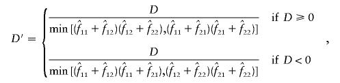 |
and
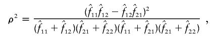 |
respectively. In the first method, the maximum-likelihood estimates,  , of the haplotype frequencies were calculated using the data for all available loci. In the second method, however, genotypic data only at the two relevant loci were used to estimate
  .
.
Results
Estimation of Haplotypes for the SAA Gene
The haplotype data from 156 subjects for six SNP loci on the SAA gene (Moriguchi et al. 2001) were used to perform haplotype estimation with our algorithm. In this data set, diplotype configurations of all the individuals have been determined, and these data were interpreted as reflecting the real data. So that this data set could be used for our algorithm, the haplotype data from different subjects were mixed together, and the phase data were removed. Using the phase-unknown genotype data at multiple linked loci, we performed haplotype estimation using our LDPooled program.
Tables 1 and 2 show the results of estimation in which each pool contained one, two, or four subjects. Table 1 shows the central-processing-unit time required, the number of iterations before convergence, the LOD scores, the χ2 values, and the P values. Each P value represents the risk for excluding the null hypothesis of independence between all six loci. As the number of subjects in each pool increased, the LOD scores and the χ2 values decreased while the P values increased (table 1). These results are probably due to the decrease in information content because of pooling.
Table 1.
Computational Data Obtained by Execution of LDPooled for SAA Data—and Results of Test of Independence for All Six Loci
| No. of Subjects in a Poola | No. of Pools | Central-Processing-Unit Time(s) | No. of Iterations | LOD Scoreb | χ2b | P |
| 1 | 156 | 11.26 | 40 | 121.3 | 558.5 | 10−82 |
| 2 | 78 | 5.93 | 142 | 75.0 | 345.5 | 10−42 |
| 4 | 39 | 30.86 | 72 | 44.5 | 204.8 | 10−17 |
Genotypic data from one, two, or four subjects were mixed to make a pool.
The methods for the calculation of the LOD score and the χ2 value were as described in the “Methods” section. The degrees of freedom should be 57, as calculated by equation (3).
Table 2.
Haplotype Frequencies Estimated Using Different Estimation Protocols for SAA Data
|
Frequency (Mean ± SD)b for |
|||
| Haplotypea | One-Subject Pool | Two-Subject Pool | Four-Subject Pool |
| ACTGCC | .394 | .406 (.40134 ± .01218) | .391 (.40547 ± .01843) |
| ACCGTC | .214 | .210 (.21079 ± .01356) | .226 (.21262 ± .02260) |
| AGCGCT | .210 | .209 (.21364 ± .01071) | .214 (.21885 ± .01868) |
| GCCGTC | .036 | .025 (.03303 ± .00937) | .022 (.02669 ± .01665) |
| GCTGCT | .035 | .040 (.03045 ± .00749) | .027 (.02583 ± .01282) |
| GGCACT | .023 | .015 (.01994 ± .00591) | .008 (.01730 ± .00968) |
| ACTGCT | .023 | .010 (.01633 ± .00710) | .023 (.01221 ± .00944) |
| AGCACT | .018 | .021 (.01849 ± .00628) | .021 (.01507 ± .00948) |
| GGCGCT | .017 | .020 (.01487 ± .00861) | .023 (.01371 ± .01525) |
| ACTGTC | .013 | .009 (.00883 ± .00395) | … (.00433 ± .00452) |
| ACCGCC | .006 | .007 (.00501 ± .00221) | .007 (.00293 ± .00277) |
| ACCATC | .006 | … (.00361 ± .00399) | … (.00275 ± .00498) |
| AGCGCC | .003 | .004 (.00274 ± .00186) | … (.00158 ± .00230) |
| GCCATC | … | .012 (.00144 ± .00319) | .014 (.00295 ± .00563) |
| ACCGTT | … | .009 (.00335 ± .00532) | … (.00412 ± .00660) |
| AGCGTT | … | .004 (.00106 ± .00267) | … (.00109 ± .00264) |
| GCTGCC | … | … (.00325 ± .00633) | .009 (.00671 ± .01207) |
| GCTACT | … | … (.00086 ± .00199) | .004 (.00176 ± .00355) |
| GCTGTT | … | … (.00044 ± .00114) | .003 (.00100 ± .00220) |
| GCCGTT | … | … (.00369 ± .00608) | … (.00744 ± .01086) |
| GCCATT | … | … (.00063 ± .00164) | … (.00109 ± .00271) |
| ACTACC | … | … (.00041 ± .00183) | … (.00103 ± .00338) |
Haplotypes with mean frequency >.001 in at least one of the estimation protocols are included.
Frequency is based on a single estimation. Mean and SD are based on different random samplings used to make the pools (for two- and four-subject pool protocols).
Table 2 shows the estimated haplotype frequencies obtained using different estimation protocols in which each pool contained genotype data from one, two, or four subjects. When each pool contained DNA from more than one subject, means and SDs of the frequencies estimated using different combinations of the subjects sampled from the original data for each subject are also shown. The results of estimation when each pool contained only one subject were exactly the same as those noted in the previous study, in which no DNA was pooled (Kitamura et al. 2002). Although the estimated haplotype frequencies varied with the numbers of subjects in a pool, they were still good estimates of the frequencies of the major haplotypes—ACTGCC, ACCGTC, and AGCGCT—as long as the number of subjects in a pool did not exceed four (table 2). For the three major haplotypes, the SDs of the estimated frequencies obtained using different random samplings to make the pools were typically <10% of the means (table 2). For minor haplotypes (frequency <0.1), however, estimation was not accurate. For example, the frequency of haplotype ACTGTC was estimated to be 0.0 by the four-subject pool estimation but 0.013 by the single-subject pool estimation; this haplotype should appear only 4 times among 156 individuals (or 312 haplotype copies) if the latter estimation is accurate.
Estimation of D and D′
Table 3 shows D and D′ values calculated from the estimated haplotype frequencies. In this case,  values, the estimated frequencies of the two-locus haplotypes, were calculated from the estimated frequencies of the six-locus haplotypes, as described in the “Methods” section. When
  values were estimated from the genotype data for the two loci, D and D′ values were very similar in some cases, but there were some cases in which the two methods yielded quite different values (data not shown). Means and SDs of the values estimated using different combinations of the subjects are shown when each pool contained more than one subject (table 3). Although the values varied between estimation protocols, they were still rather consistent, as long as the number of subjects in a pool did not exceed four and |D| was >0.1. However, in some cases, the SDs of the estimated D and D′ values obtained using different random samplings to make the pools were almost 50% of the means, and the values estimated by different estimation protocols differed greatly. The accuracy of the estimation of D′ is heavily dependent on the allele frequency. The minor-allele frequencies were 0.11 at locus 1 and 0.05 at locus 4. The SDs of the estimated D′ values for the locus pairs including one of these loci were larger than those for the other locus pairs. Thus, when the minor-allele frequency is low, the estimated D′ value obtained using pooled genotype data is not accurate.
Table 3.
Estimated D and D′ for SAA Data
|
Da for One-Subject Pool, at Locus |
|||||
| Locus | 2 | 3 | 4 | 5 | 6 |
| 1 | .010 | −.017 | −.018 | .006 | .039 |
| 2 | −.127 | −.029 | −.073 | .180 | |
| 3 | .022 | −.112 | −.094 | ||
| 4 | .006 | −.026 | |||
| 5 | −.088 | ||||
|
D′a for One-Subject Pool, at Locus |
|||||
| Locus | 2 | 3 | 4 | 5 | 6 |
| 1 | .124 | −.323 | −.418 | .073 | .521 |
| 2 | −1.000 | −.815 | −1.000 | .981 | |
| 3 | 1.000 | −.897 | −.619 | ||
| 4 | .500 | −.800 | |||
| 5 | −1.000 | ||||
|
D (Mean ± SD)a for Two-Subject Pool, at Locus |
|||||
| Locus | 2 | 3 | 4 | 5 | 6 |
| 1 | .004 (.005 ± .010) | −.012 (−.014 ± .010) | −.022 (−.019 ± .004) | .007 (.010 ± .012) | .038 (.035 ± .010) |
| 2 | −.127 (−.126 ± .002) | −.023 (−.026 ± .005) | −.069 (−.071 ± .003) | .179 (.180 ± .001) | |
| 3 | .022 (.019 ± .004) | −.116 (−.115 ± .003) | −.103 (−.102 ± .009) | ||
| 4 | .001 (.006 ± .005) | −.020 (−.025 ± .005) | |||
| 5 | −.075 (−.077 ± .009) | ||||
|
D′ (Mean ± SD)a for Two-Subject Pool, at Locus |
|||||
| Locus | 2 | 3 | 4 | 5 | 6 |
| 1 | .053 (.013 ± .215) | −.235 (−.279 ± .197) | −.506 (−.437 ± .092) | .088 (.091 ± .202) | .502 (.465 ± .138) |
| 2 | −1.000 (−.994 ± .014) | −.648 (−.738 ± .156) | −.945 (−.977 ± .040) | .979 (.982 ± .007) | |
| 3 | 1.000 (.880 ± .165) | −.928 (−.916 ± .027) | −.675 (−.671 ± .057) | ||
| 4 | .050 (.479 ± .334) | −.620 (−.775 ± .154) | |||
| 5 | −.851 (−.880 ± .103) | ||||
|
D (Mean ± SD)a for Four-Subject Pool, at Locus |
|||||
| Locus | 2 | 3 | 4 | 5 | 6 |
| 1 | .001 (.003 ± .016) | −.008 (−.014 ± .018) | −.022 (−.020 ± .007) | .010 (.011 ± .020) | .030 (.034 ± .016) |
| 2 | −.120 (−.125 ± .003) | −.016 (−.021 ± .009) | −.070 (−.070 ± .003) | .180 (.180 ± .002) | |
| 3 | .018 (.016 ± .006) | −.119 (−.117 ± .004) | −.091 (−.107 ± .014) | ||
| 4 | −.001 (.004 ± .008) | −.018 (−.022 ± .008) | |||
| 5 | −.082 (−.070 ± .013) | ||||
|
D′ (Mean ± SD)a for Four-Subject Pool, at Locus |
|||||
| Locus | 2 | 3 | 4 | 5 | 6 |
| 1 | .009 (−.064 ± .330) | −.152 (−.266 ± .326) | −.514 (−.467 ± .174) | .118 (.068 ± .366) | .394 (.454 ± .216) |
| 2 | −.948 (−.985 ± .024) | −.460 (−.595 ± .273) | −.956 (−.963 ± .048) | .982 (.982 ± .013) | |
| 3 | .800 (.743 ± .279) | −.948 (−.932 ± .034) | −.598 (−.706 ± .089) | ||
| 4 | −.042 (.385 ± .451) | −.554 (−.688 ± .268) | |||
| 5 | −.927 (−.793 ± .153) | ||||
D or D′ value is based on a single estimation. Mean and SD are based on different random samplings.
Table 4 shows the results of estimation of the combination of haplotype copies in each DNA pool. For each protocol, only the portion of the data corresponding to the first 12 subjects is shown. The results indicate that, in many of the pools, the posterior probabilities of the combinations of haplotype copies with the highest probabilities were 1 or nearly 1. When the contents of the estimated combinations of haplotype copies were carefully compared, they were found in many cases to be consistent between different estimation protocols. For example, the contents of pool number 1 in the two-subject pool protocol should be the same as the combination of pool numbers 1 and 2 in the one-subject pool protocol. Table 4 shows that this was indeed the case. In other cases, however, the contents of a pool estimated by a protocol were inconsistent with those in the pools estimated by a different protocol.
Table 4.
Estimation of Haplotype Combination in Each DNA Pool for the SAA Gene
| Pool No. | CombinationNo. | Pra | Haplotype Combination |
| One-subject pools: | |||
| 1 | 1 | 1.000 | ACTGCC AGCGCT |
| 2 | 1 | 1.000 | AGCGCT AGCGCT |
| 3 | 1 | 1.000 | ACTGCC AGCGCT |
| 4 | 1 | 1.000 | ACCGTC ACTGCC |
| 5 | 1 | 1.000 | ACCGTC ACTGCC |
| 6 | 1 | .997 | AGCGCT GCTGCT |
| 2 | .003 | ACTGCT GGCGCT | |
| 7 | 1 | 1.000 | ACTGCC AGCGCT |
| 8 | 1 | 1.000 | ACCGTC ACCGTC |
| 9 | 1 | 1.000 | AGCGCT AGCGCT |
| 10 | 1 | .988 | ACCGTC GCTGCT |
| 2 | .012 | ACTGCT GCCGTC | |
| 11 | 1 | 1.000 | ACTGCC ACTGCC |
| 12 | 1 | .982 | ACCGTC GGCACT |
| 2 | .018 | AGCACT GCCGTC | |
| 3 | .001 | ACCATC GGCGCT | |
| Two-subject pools: | |||
| 1 | 1 | 1.000 | ACTGCC AGCGCT AGCGCT AGCGCT |
| 2 | 1 | 1.000 | ACCGTC ACTGCC ACTGCC AGCGCT |
| 3 | 1 | .995 | ACCGTC ACTGCC AGCGCT GCTGCT |
| 2 | .002 | ACCGTC ACTGCC ACTGCT GGCGCT | |
| 3 | .001 | ACTGCC ACTGCT AGCGCT GCCGTC | |
| 4 | .001 | ACCGTT ACTGCC ACTGCC GGCGCT | |
| 4 | 1 | 1.000 | ACCGTC ACCGTC ACTGCC AGCGCT |
| 5 | 1 | .993 | ACCGTC AGCGCT AGCGCT GCTGCT |
| 2 | .005 | ACCGTC ACTGCT AGCGCT GGCGCT | |
| 3 | .002 | ACTGCT AGCGCT AGCGCT GCCGTC | |
| 6 | 1 | .581 | ACCGTC ACTGCC ACTGCC GGCACT |
| 2 | .402 | ACTGCC ACTGCC AGCGCT GCCATC | |
| 3 | .017 | ACTGCC ACTGCC AGCACT GCCGTC | |
| Four-subject pools: | |||
| 1 | 1 | 1.000 | ACCGTC ACTGCC ACTGCC ACTGCC AGCGCT AGCGCT AGCGCT AGCGCT |
| 2 | 1 | .941 | ACCGTC ACCGTC ACCGTC ACTGCC ACTGCC AGCGCT AGCGCT GCTGCT |
| 2 | .028 | ACCGTC ACCGTC ACCGTC ACTGCC ACTGCC ACTGCT AGCGCT GGCGCT | |
| 3 | .025 | ACCGTC ACCGTC ACTGCC ACTGCC ACTGCT AGCGCT AGCGCT GCCGTC | |
| 4 | .006 | ACCGTC ACCGTC ACCGTC ACTGCC ACTGCT AGCGCT AGCGCT GCTGCC | |
| 3 | 1 | .415 | ACCGTC ACTGCC ACTGCC AGCGCT AGCGCT AGCGCT GCCATC GCTGCT |
| 2 | .262 | ACCGTC ACCGTC ACTGCC ACTGCC AGCGCT AGCGCT GCTGCT GGCACT | |
| 3 | .077 | ACCGTC ACTGCC ACTGCC AGCGCT AGCGCT AGCGCT GCCGTC GCTACT | |
| 4 | .073 | ACCGTC ACCGTC ACTGCC ACTGCC AGCGCT AGCGCT GCTACT GGCGCT | |
| 5 | .039 | ACCGTC ACTGCC ACTGCC AGCGCT AGCGCT AGCACT GCCGTC GCTGCT | |
| 6 | .037 | ACCGTC ACCGTC ACTGCC ACTGCC AGCGCT AGCACT GCTGCT GGCGCT | |
| 7 | .020 | ACTGCC ACTGCC ACTGCT AGCGCT AGCGCT AGCGCT GCCGTC GCCATC | |
| 8 | .019 | ACCGTC ACTGCC ACTGCC ACTGCT AGCGCT AGCGCT GCCATC GGCGCT | |
| 9 | .015 | ACCGTC ACCGTC ACTGCC AGCGCT AGCGCT AGCGCT GCTGCC GCTACT | |
| 10 | .012 | ACCGTC ACTGCC ACTGCC ACTGCT AGCGCT AGCGCT GCCGTC GGCACT | |
| 11 | .012 | ACCGTC ACCGTC ACTGCC ACTGCC ACTGCT AGCGCT GGCGCT GGCACT | |
| 12 | .008 | ACCGTC ACCGTC ACTGCC AGCGCT AGCGCT AGCACT GCTGCC GCTGCT | |
| 13 | .004 | ACCGTC ACTGCC ACTGCT AGCGCT AGCGCT AGCGCT GCCATC GCTGCC | |
| 14 | .002 | ACCGTC ACCGTC ACTGCC ACTGCT AGCGCT AGCGCT GCTGCC GGCACT | |
| 15 | .002 | ACTGCC ACTGCC ACTGCT AGCGCT AGCGCT AGCACT GCCGTC GCCGTC | |
| 16 | .002 | ACCGTC ACTGCC ACTGCC ACTGCT AGCGCT AGCACT GCCGTC GGCGCT | |
| 17 | .002 | ACCGTC ACCGTC ACTGCC ACTGCC ACTGCT AGCACT GGCGCT GGCGCT |
Posterior probability, given the estimated haplotype frequencies, of each haplotype combination for a pool.
Bootstrap Method to Calculate SEs of the Estimated Haplotype Frequencies
Since the estimated haplotype frequencies exhibited errors, we implemented in LDPooled the algorithm to calculate SEs by the bootstrap method. Using the same data for the SAA gene from 156 subjects, we made one-, two-, or four-subject pools, as described above (see the “Estimation of Haplotypes for the SAA Gene” subsection). We then applied the bootstrap method to such data, as described in the “Methods” section. Figure 1 shows the means and SEs of the estimated haplotype frequencies obtained using different estimation protocols (one-, two-, and four-subject pools). Bootstrap sampling was repeated 10,000 times for each estimation protocol. As shown, the estimated frequencies were rather stable for haplotypes ACTGCC, ACCGTC, and AGCGCT, irrespective of the number of subjects in a pool. The lengths of the error bars were rather short, compared with those of the mean values for these haplotypes. In addition, the means of the haplotype frequencies estimated by different protocols were approximately the same for the same haplotypes. For the minor haplotypes (pi<0.1), however, the frequencies estimated by the different protocols varied significantly, and the error bars were rather long, compared with the mean values (fig. 1). For some minor haplotypes, the error bars were too large to be tolerated when two- and four-subject pools were used. When the total numbers of the subjects were the same, the estimated haplotype frequencies obtained using two- and four-subject pools for such minor haplotypes were less accurate than the frequencies estimated using one-subject pools.
Figure 1.

Means and SEs of estimated haplotype frequencies calculated by the bootstrap method for the SAA gene. Means and SEs of estimated frequencies were calculated as described in the “Methods” section.
Time and Memory Required for Calculation
The time and memory required for each calculation were recorded. When a computer with a Pentium III 1-GHz processor and a memory of 1.5 GB was used, the number of subjects within a pool was, at maximum, six when the number of loci was six. If the number of loci was 13, then the maximum number of subjects in a pool could be only two. In contrast, 25 loci were possible when no pooling was performed on DNA samples. This is because the algorithm implemented in LDPooled uses possible combinations of haplotype copies in each DNA pool and this step consumes a large amount of memory. The number of combinations increases by a power function of the number of alleles at a locus, and it increases by a factorial of the number of subjects in a pool. Therefore, the dependence of time and memory on those factors is due to the requirement of space for combinations.
Estimation of Haplotypes for the MTHFR Gene
The MTHFR gene encodes the methylenetetrahydrofolate reductase enzyme, which is related to folate metabolism. We have published data, for a total of 80 subjects, in which two linked loci of the gene are involved (Urano et al. 2002). These published data were used to make DNA pools and to estimate parameters from the pooled data. Table 5 shows estimated haplotype frequencies and means and SDs of the estimated haplotype frequencies obtained using different combinations of the subjects sampled from the original data for each subject (when the protocol for pools of two or more subjects is used) for the MTHFR gene. These data indicate that the estimated haplotype frequencies were rather accurate, even when the four-subject protocol was used. This is probably because linkage disequilibrium is very strong for this pair of loci. The data also indicate that estimation was rather accurate for haplotypes whose relative frequencies were >0.1.
Table 5.
Haplotype Frequencies Estimated Using Different Estimation Protocols for the MTHFR Gene
|
Frequency (Mean ± SD)a for |
|||
| Haplotype | One-Subject Pool | Two-Subject Pool | Four-Subject Pool |
| CA | .450 | .463 (.47038 ± .02383) | .450 (.48188 ± .03560) |
| TA | .394 | .381 (.37343 ± .02388) | .394 (.36193 ± .03566) |
| CC | .156 | .143 (.13579 ± .02373) | .156 (.12429 ± .03556) |
| TC | … | .013 (.02038 ± .02383) | … (.03187 ± .03561) |
Frequency is based on a single estimation. Mean and SD are based on different random samplings used to make the pools (for two- and four-subject pool protocols).
Figure 2 shows the results of the application of the bootstrap method to the haplotype data for the MTHFR gene. These results suggest that our method can accurately estimate haplotype frequencies for the MTHFR gene when haplotype frequencies are rather high.
Figure 2.

Means and SEs of estimated haplotype frequencies calculated by the bootstrap method for the MTHFR gene. Means and SEs of estimated frequencies were calculated as described in the “Methods” section.
D and D′ values calculated from the estimated haplotype frequencies for the MTHFR gene are shown in table 6. For the data from two- and four-subject pool protocols, means and SDs for different random samplings are also shown. These data also show that the variability of estimated values is large. If the minor-allele frequency at one of the 2 loci was low, then the estimated D′ value was not accurate, even when one-subject pools were used for estimation. Since the minor-allele frequencies were 0.39 and 0.16 at loci 1 and 2 for the MTHFR gene, SDs for D′ showed large values.
Table 6.
Estimated D and D′ for the MTHFR Gene
| D (Mean ± SD)a | D′ (Mean ± SD)a | |
| One-subject pool | −.062 | −1.000 |
| Two-subject pool | −.049 (−.041 ± .024) | −.790 (−.678 ± .370) |
| Four-subject pool | −.061 (−.029 ± .036) | −.997 (−.509 ± .513) |
D or D′ value is based on a single estimation. Mean and SD are based on different random samplings.
Estimation of Haplotypes for the NAT2 Gene
The NAT2 gene encodes the N-acetyltransferase 2 enzyme, which is related to transfer of N-acetyl residues. We have published data, for a total of 116 subjects, in which seven linked loci of the gene are involved (Tanaka et al. 2002). These published data were used to make DNA pools and to estimate parameters from the pooled data. Table 7 shows estimated haplotype frequencies and the means and SDs of the estimated haplotype frequencies obtained using different combinations of the subjects sampled from the original data for each subject (when the protocol for pools of two or more subjects is used) for the NAT2 gene. Figure 3 shows the results of the application of the bootstrap method to the haplotype data for the NAT2 gene. These results show that our method can accurately estimate haplotype frequencies when the frequencies of the haplotypes for the NAT2 gene are rather high (>0.1). For minor haplotypes (<0.1), when two- and four-subject pools were used, the error bars were too large to be tolerated.
Table 7.
Haplotype Frequencies Estimated Using Different Estimation Protocols for the NAT2 Gene
|
Frequency (Mean ± SD)b for |
|||
| Haplotypea | One-Subject Pool | Two-Subject Pool | Four-Subject Pool |
| GCTCGAG | .711 | .720 (.71440 ± .00294) | .720 (.71635 ± .00299) |
| GTTCAAG | .185 | .185 (.18363 ± .00190) | .185 (.18404 ± .00181) |
| GTTCGAA | .091 | .082 (.08937 ± .00257) | .082 (.08700 ± .00315) |
| GTTCGAG | .004 | .004 (.00392 ± .00057) | .004 (.00378 ± .00092) |
| GCCTGGG | .004 | … (.00192 ± .00200) | … (.00116 ± .00182) |
| GCCCAAG | .004 | … (.00324 ± .00157) | … (.00222 ± .00199) |
| GTCTGGA | … | .004 (.00068 ± .00150) | .004 (.00167 ± .00197) |
| GTCCAAA | … | .004 (.00066 ± .00148) | .004 (.00159 ± .00196) |
| GTCTAGG | … | … (.00132 ± .00188) | … (.00097 ± .00171) |
Haplotypes with mean frequency >.001 in at least one of the estimation protocols are included.
Frequency is based on a single estimation. Mean and SD are based on different random samplings used to make the pools (for two- and four-subject pool protocols).
Figure 3.

Means and SEs of estimated haplotype frequencies calculated by the bootstrap method for the NAT2 gene. Means and SEs of estimated frequencies were calculated as described in the “Methods” section.
D and D′ values calculated from the estimated haplotype frequencies for the NAT2 gene are shown in table 8. Compared with the results of the one-subject pool, some D′ values for two- or four-subject pools showed the opposite signs. The minor-allele frequencies at loci 3, 4, 6, and 7 were <0.1. When the minor-allele frequency is very low, estimated values obtained using pooled genotype data are not accurate for D′.
Table 8.
Estimated D and D′ for the NAT2 Gene
|
Da for One-Subject Pool, at Locus |
||||||
| Locus | 2 | 3 | 4 | 5 | 6 | 7 |
| 1 | .000 | .000 | .000 | .000 | .000 | .000 |
| 2 | .002 | −.001 | −.132 | −.001 | −.065 | |
| 3 | −.004 | .003 | −.004 | −.001 | ||
| 4 | .001 | .004 | .000 | |||
| 5 | .001 | −.017 | ||||
| 6 | .000 | |||||
|
D′a for One-Subject Pool, at Locus |
||||||
| Locus | 2 | 3 | 4 | 5 | 6 | 7 |
| 1 | .000 | .000 | .000 | .000 | .000 | .000 |
| 2 | 1.000 | −1.000 | −.968 | −1.000 | −1.000 | |
| 3 | −1.000 | .383 | −1.000 | −1.000 | ||
| 4 | 1.000 | 1.000 | 1.000 | |||
| 5 | 1.000 | −1.000 | ||||
| 6 | 1.000 | |||||
|
Da for Two-Subject Pool, at Locus |
||||||
| Locus | 2 | 3 | 4 | 5 | 6 | 7 |
| 1 | .000 (.000 ± .000) | .000 (.000 ± .000) | .000 (.000 ± .000) | .000 (.000 ± .000) | .000 (.000 ± .000) | .000 (.000 ± .000) |
| 2 | −.006 (−.001 ± .003) | .003 (.001 ± .002) | −.137 (−.133 ± .002) | .003 (.001 ± .002) | −.065 (−.065 ± .000) | |
| 3 | −.004 (−.004 ± .000) | .003 (.004 ± .002) | −.004 (−.004 ± .000) | .008 (.001 ± .003) | ||
| 4 | .001 (−.000 ± .002) | .004 (.004 ± .000) | −.004 (−.001 ± .002) | |||
| 5 | .001 (−.000 ± .002) | −.013 (−.016 ± .001) | ||||
| 6 | −.004 (−.001 ± .002) | |||||
|
D′a for Two-Subject Pool, at Locus |
||||||
| Locus | 2 | 3 | 4 | 5 | 6 | 7 |
| 1 | .000 (.000 ± .000) | .000 (.000 ± .000) | .000 (.000 ± .000) | .000 (.000 ± .000) | .000 (.000 ± .000) | .000 (.000 ± .000) |
| 2 | −1.000 (.135 ± .720) | 1.000 (.054 ± .999) | −1.000 (−.974 ± .012) | 1.000 (.054 ± .999) | −1.000 (−1.000 ± .000) | |
| 3 | −1.000 (−1.000 ± .000) | .383 (.583 ± .289) | −1.000 (−1.000 ± .000) | 1.000 (−.511 ± .711) | ||
| 4 | 1.000 (.352 ± .936) | 1.000 (1.000 ± .000) | −1.000 (.614 ± .790) | |||
| 5 | 1.000 (.352 ± .936) | −.749 (−.959 ± .093) | ||||
| 6 | −1.000 (.614 ± .790) | |||||
|
Da for Four-Subject Pool, at Locus |
||||||
| Locus | 2 | 3 | 4 | 5 | 6 | 7 |
| 1 | .000 (.000 ± .000) | .000 (.000 ± .000) | .000 (.000 ± .000) | .000 (.000 ± .000) | .000 (.000 ± .000) | .000 (.000 ± .000) |
| 2 | −.006 (−.002 ± .003) | .003 (.002 ± .002) | −.137 (−.134 ± .002) | .003 (.002 ± .002) | −.065 (−.065 ± .000) | |
| 3 | −.004 (−.004 ± .000) | .003 (.004 ± .002) | −.004 (−.004 ± .000) | .008 (.003 ± .003) | ||
| 4 | .001 (.000 ± .002) | .004 (.004 ± .000) | −.004 (−.002 ± .002) | |||
| 5 | .001 (.000 ± .002) | −.013 (−.015 ± .002) | ||||
| 6 | −.004 (−.002 ± .002) | |||||
|
D′a for Four-Subject Pool, at Locus |
||||||
| Locus | 2 | 3 | 4 | 5 | 6 | 7 |
| 1 | .000 (.000 ± .000) | .000 (.000 ± .000) | .000 (.000 ± .000) | .000 (.000 ± .000) | .000 (.000 ± .000) | .000 (.000 ± .000) |
| 2 | −1.000 (−.259 ± .670) | 1.000 (.286 ± .959) | −1.000 (−.982 ± .016) | 1.000 (.286 ± .959) | −1.000 (−1.000 ± .000) | |
| 3 | −1.000 (−1.000 ± .000) | .383 (.524 ± .275) | −1.000 (−1.000 ± .000) | 1.000 (.032 ± .777) | ||
| 4 | 1.000 (.504 ± .864) | 1.000 (1.000 ± .000) | −1.000 (.220 ± .976) | |||
| 5 | 1.000 (.504 ± .864) | −.749 (−.895 ± .124) | ||||
| 6 | −1.000 (.220 ± .976) | |||||
D or D′ value is based on a single estimation. Mean and SD are based on different random samplings.
Estimation of Haplotypes for the Smoothelin Gene
Estimation of haplotype frequencies and combination of haplotype copies within each pool was performed using data for the smoothelin gene. The set of all data includes the genotype data from 32 black, 90 white, and 102 Japanese subjects; however, this set will be published later, and the present article used the data from Japanese subjects only, to test the function of LDPooled.
The typed loci spanned an ∼300-kb region and contained both SNP and microsatellite polymorphisms. The total number of SNP loci, including insertion/deletion polymorphisms, was 36. Since the number of loci was too large to estimate the haplotypes by using the EM algorithm, the loci were selected to reduce the number as follows: First, the SNP loci with minor-allele frequencies that were not <0.2 were selected; the number of SNP loci was still too large for the haplotype estimation with pooled DNA. Then, linkage-disequilibrium measures D′ and ρ2 were calculated for each of those SNP pairs, a haplotype block containing nine loci was determined, and the nine loci were used for the haplotype estimation; the same haplotype block was determined for two different protocols, one by the one-subject pool method and the other by the two-subject pool method. Finally, the haplotype estimation and SE calculation by the bootstrap method were performed for the nine loci data; bootstrap sampling was repeated 10,000 times for each estimation protocol. All these processes were performed using our LDPooled program.
Figure 4 shows a comparison of the estimated haplotype frequencies, as well as the SEs, by the application of the bootstrap method between two different protocols. As shown, the haplotype frequencies estimated by the two protocols were quite similar as long as haplotype frequencies were >0.1. Even for minor haplotypes, the frequencies estimated using two different protocols were similar, except when the haplotype frequencies were <0.01. However, the error bars were rather long, compared with the mean values for these minor haplotypes. Thus, the calculation of SEs by the bootstrap method was useful for the evaluation of the inaccuracy of estimated haplotype frequencies.
Figure 4.

Means and SEs of estimated haplotype frequencies calculated by the bootstrap method for the smoothelin gene. Means and SEs of estimated frequencies were calculated as described in the “Methods” section.
Estimation of Pairwise Linkage-Disequilibrium Measure ρ2
The strength of linkage disequilibrium is usually measured in pairwise fashion. We calculated ρ2 as described in the “Methods” section. Figure 5 shows estimated ρ2 values for all  pairs. In this case,
  values were estimated using only two-locus genotype data. Although slight differences were observed, the ρ2 values estimated by the two different protocols (i.e., single-subject pool and two-subject pool) were quite similar. The mean and the SD for the estimated ρ2 values for different SNP pairs were 0.114 and 0.224, respectively, with the one-subject pool protocol, and 0.118 and 0.227, respectively, with the two-subject pool protocol. The mean and the SD of the absolute value of the difference between estimated ρ2 values were 0.011 and 0.022, respectively. On average, the absolute value of the difference in estimated ρ2 values obtained by the two protocols was ∼9.5% of the mean.
Figure 5.

Distribution of ρ2 values estimated for different estimation protocols for the smoothelin gene in Japanese
Discussion
Genotyping is usually performed on DNA samples obtained from single subjects. In special cases, however, samples from different subjects are mixed, and genotyping is performed on the mixed samples. For example, DNA samples are mixed, and the number of allele copies in each mixed sample is determined for case and control samples, to reduce the cost of genotyping. Recently, case-control studies in which allele frequencies are compared between different groups have been performed at thousands of loci in numerous subjects (Barcellos et al. 1997; Collins et al. 2000). If the objective of studies is only to detect differences in the frequencies of alleles between case and control groups, then the pooled DNA method can be efficient, as long as the frequencies can be determined accurately for the pooled samples. However, phase information becomes ambiguous with pooling.
The question that we addressed when beginning the present study was the following: If we wish to know either the phase of each subject, haplotype frequencies in the population, numbers of haplotype copies in the sample, or the strength of linkage disequilibrium for a group of linked loci, how accurately can we make such estimations when using pooled DNA data? More specifically, how accurately can we estimate either the phase of each subject, haplotype frequencies in the population, numbers of haplotype copies in the sample, or the strength of linkage disequilibrium when only data for the allele copies in each pooled sample containing M different subjects are available? If M=1, then this is equivalent to the procedure for estimating the frequencies of haplotypes by the EM algorithm when using nonpooled samples.
In certain cases, the regular EM algorithm to estimate the frequencies of haplotypes under the assumption of Hardy-Weinberg equilibrium by using genotypic data is also considered to be a method to estimate the parameters by using data from pooled samples. In the regular method, however, pooling of haplotypes is performed during fertilization, whereas, in our method, it is performed in vitro. Our method is useful for the estimation of various linkage-disequilibrium parameters on the basis of incomplete information from pooled haplotype samples, each of which contains 2M haplotype copies. It should be noted that Hardy-Weinberg equilibrium is always assumed in our method, as well as in the regular method. In addition, our method requires that pooling of DNA be performed at random.
As expected, information becomes degenerated as the number of haplotype copies in a pool increases. Thus, LOD scores and χ2 values for testing the independence of all the loci decreased when the number of subjects whose DNA was mixed in a pool increased. Naturally, P values for testing of independence increased.
We used real data from subjects, rather than simulated data, to test our method, since no standard simulation method is available for haplotypes and linkage disequilibrium. Naturally, the number of sets of samples that we tested is insufficient to extend the results obtained in the present study to other sets of data.
Our results from a limited number of sets of samples suggested that the estimation of frequencies of haplotypes was rather accurate when frequencies were >0.1 and when fewer than four subjects' data were in a pool. As total numbers of subjects in a data set, we tested the data from 156, 80, 116, and 102 subjects. In addition, our data were for 2–13 loci. Many other cases featuring various total numbers of subjects, various numbers of loci, and various degrees of linkage disequilibrium should be examined. However, our data suggest that the frequencies of haplotypes with frequencies of >0.1 can be accurately estimated from pooled DNA data under some conditions.
We examined the variability of estimated frequencies by using different combinations of the original samples. This method was useful for estimating such variability, but, of course, it cannot be applied to the real pooled DNA data since, in the latter case, data for single subjects are not available. To evaluate variability in haplotype frequencies estimated from real pooled DNA data, we used the bootstrap method to calculate means and SEs. The SE for each haplotype frequency was consistent with the SD obtained from the frequencies estimated from different combinations of the DNA samples—that is, it was small when the haplotype frequency was >0.1. Therefore, our bootstrap method is likely to be useful for the estimation of variability in estimated haplotype frequency, although it features some limitations.
Note that the objective of the haplotype-frequency estimation is often not to estimate the proportions of the haplotypes in the sample but to estimate the population frequencies. Therefore, there are two different sources of inaccuracy for the haplotype frequency estimation: one is from the sampling of the haplotypes from the population, and the other is from the estimation using the sample data. The inaccuracy from the sampling is high when the sample size is small. Thus, the sample with a larger size represents more accurately the information in the population than a sample with a smaller size. Therefore, there are situations in which the analysis based on MN-subject data, from N pools composed of M subjects, is better than the analysis based on N-subject data, from N pools composed of a single subject.
Estimation of linkage-disequilibrium measures such as D and D′ was performed using pooled DNA data. Compared to the results of the haplotype-frequency estimation, variability in the estimated D′ value was large, especially when the minor-allele frequencies were <0.16 at one of the loci. When the minor-allele frequencies were high, the estimated D′ values obtained using two- or four-subject pools were in good agreement with the results of one-subject pools, and the SDs of the D′ values were rather small, compared with the means. In contrast, ρ2 was better than D and D′ when the data from a large number of linked loci were analyzed for the purpose of observing the gross pattern of linkage disequilibrium (unpublished data). The gross pattern of the linkage-disequilibrium measure ρ2 could be reliably reproduced when the two-subject protocol was used.
Our LDPooled program has a limitation in that it cannot handle missing data, even though such a function has been included in haplotype-estimation programs. The reason for this inability is that, for the pooled DNA data, the number of possible events becomes too large to be handled by current machines. We still work for the implementation of this function, but this needs extended expansion of the memory and calculation speed of computers.
Thus, although more data sets should be analyzed, our methods for the estimation of haplotype frequencies and linkage-disequilibrium parameters may be useful when genotype data from pooled DNA samples are available. The present method may also be useful when the haplotype is to be estimated in a sample in which DNA from more than one person is mixed. Such cases may occur in the fields of forensic medicine and archaeology. As shown, the posterior distribution of combinations of haplotype copies can be estimated given the estimated population haplotype frequencies. In the near future, the frequencies of the major haplotypes for each haplotype block (Gabriel et al. 2002) in ethnic groups may be determined. By use of such data, the haplotype copies in pooled DNA samples may be estimated.
In summary, we have devised a new method to estimate haplotype frequencies, combinations of haplotype copies, and the D, D′, and ρ2 values from the pooled DNA data, and we have implemented the algorithm obtained by the computer program LDPooled. We have also used the bootstrap method to calculate SEs of the estimated frequencies. Although the frequencies of haplotypes can be estimated rather accurately when the frequencies are >0.1, the estimated data for haplotypes with lower frequencies were not reliable, as shown by the large error bars calculated by the bootstrap method. Estimated D and D′ values exhibited large variation except when |D| values were >0.1. The gross pattern of the linkage-disequilibrium measure ρ2 may be reproduced using the two-subject pool protocol for numerous linked loci.
Acknowledgment
The present study was supported by grants from the New Energy and Industrial Technology Development Organization.
References
- Barcellos LF, Klitz W, Field LL, Tobias R, Bowcock AM, Wilson R, Nelson MP, Nagatomi J, Thomson G (1997) Association mapping of disease loci, by use of pooled DNA genomic screen. Am J Hum Genet 61:734–747 [DOI] [PMC free article] [PubMed] [Google Scholar]
- Clark AG (1990) Inference of haplotypes from PCR-amplified samples of diploid populations. Mol Biol Evol 7:111–122 [DOI] [PubMed] [Google Scholar]
- Collins HE, Li H, Inda SE, Anderson J, Laiho K, Toumilehto J, Seldin MF (2000) A simple and accurate method for determination of microsatellite total allele content differences between DNA pools. Hum Genet 106:218–226 [DOI] [PubMed] [Google Scholar]
- Excoffier L, Slatkin M (1995) Maximum-likelihood estimation of molecular haplotype frequencies in a diploid population. Mol Biol Evol 12:921–927 [DOI] [PubMed] [Google Scholar]
- Fallin D, Schork NJ (2000) Accuracy of haplotype frequency estimation for biallelic loci, via the expectation-maximization algorithm for unphased diploid genotype data. Am J Hum Genet 66:216–234 [DOI] [PMC free article] [PubMed] [Google Scholar]
- Gabriel SB, Schaffner SF, Nguyen H, Moore JM, Roy J, Blumenstiel B, Higgins J, DeFelice M, Lochner A, Faggart M, Liu-Cordero SN, Rotimi C, Adeyemo A, Cooper R, Ward R, Lander ES, Daly MJ, Altshuler D (2002) The structure of haplotype blocks in the human genome. Science 296:2225–2229 [DOI] [PubMed] [Google Scholar]
- Hawley M, Kidd K (1995) HAPLO: a program using the EM algorithm to estimate the frequencies of multi-site haplotypes. J Hered 86:409–411 [DOI] [PubMed] [Google Scholar]
- Hodge SE, Boehnke M, Spence MA (1999) Loss of information due to ambiguous haplotyping of SNPs. Nat Genet 21:360–361 [DOI] [PubMed] [Google Scholar]
- Judson R, Stephens JC, Windemuth A (2000) The predictive power of haplotypes in clinical response. Pharmacogenomics 1:5–16 [DOI] [PubMed] [Google Scholar]
- Kitamura Y, Moriguchi M, Kaneko H, Morisaki H, Morisaki T, Toyama K, Kamatani N (2002) Determination of probability distribution of diplotype configuration (diplotype distribution) for each subject from genotypic data using the EM algorithm. Ann Hum Genet 66:183–193 [DOI] [PubMed] [Google Scholar]
- Kruglyak L, Daly MJ, Reeve-Daly MP, Lander ES (1996) Parametric and nonparametric linkage analysis: a unified multipoint approach. Am J Hum Genet 58:1347–1363 [PMC free article] [PubMed] [Google Scholar]
- Kruglyak L (1999) Prospects for whole-genome linkage disequilibrium mapping of common disease genes. Nat Genet 22:139–144 [DOI] [PubMed] [Google Scholar]
- Lathrop GM, Lalouel JM, Julier C, Ott J (1985) Multilocus linkage analysis in humans: detection of linkage and estimation of recombination. Am J Hum Genet 37:482–498 [PMC free article] [PubMed] [Google Scholar]
- Lewontin RC (1964) The interaction of selection and linkage. I. General considerations: heterotic models. Genetics 49:49–67 [DOI] [PMC free article] [PubMed] [Google Scholar]
- Long JC, Williams RC, Urbanek M (1995) An E-M algorithm and testing strategy for multiple locus haplotypes. Am J Hum Genet 56:799–810 [PMC free article] [PubMed] [Google Scholar]
- Martin ER, Gilbert JR, Lai EH, Riley J, Rogala AR, Slotterbeck BD, Sipe CA, Grubber JM, Warren LL, Conneally PM, Saunders AM, Schmechel DE, Purvis I, Pericak-Vance MA, Roses AD, Vance JM (2000) Analysis of association at single nucleotide polymorphisms in the APOE region. Genomics 63:7–12 [DOI] [PubMed] [Google Scholar]
- Moriguchi M, Terai C, Kaneko H, Koseki Y, Kajiyama H, Uesato M, Inada S, Kamatani N (2001) A novel single-nucleotide polymorphism at the 5′-flanking region of SAA1 associated with risk of type AA amyloidosis secondary to rheumatoid arthritis. Arthritis Rheum 44:1266–1272 [DOI] [PubMed] [Google Scholar]
- Rieder MJ, Taylor SL, Clark AG, Nickerson DA (1999) Sequence variation in the human angiotensin converting enzyme. Nat Genet 22:59–62 [DOI] [PubMed] [Google Scholar]
- Risch N, Merikangas K (1996) The future of genetics studies of complex human diseases. Science 273:1516–1517 [DOI] [PubMed] [Google Scholar]
- Stephens M, Smith NJ, Donnelly P (2001) A new statistical method for haplotype reconstruction from population data. Am J Hum Genet 68:978–989 [DOI] [PMC free article] [PubMed] [Google Scholar]
- Tanaka E, Taniguchi A, Urano W, Nakajima H, Matsuda Y, Kitamura Y, Saito M, Yamanaka H, Saito T, Kamatani N (2002) Adverse effects of sulphasalazine in rheumatoid arthritis patients are associated with diplotype configuration at N-acetyltransferase 2 gene. J Rheumatol 29:2492–2499 [PubMed] [Google Scholar]
- Templeton AR (1999) Uses of evolutionary theory in the Human Genome Project. Annu Rev Ecol Syst 30:23–49 [Google Scholar]
- Urano W, Taniguchi A, Yamanaka H, Tanaka E, Nakajima H, Matsuda Y, Akama H, Kitamura Y, Kamatani N (2002) Polymorphisms in the methylenetetrahydrofolate reductase gene were associated with both the efficacy and the toxicity of methotrexate used for the treatment of rheumatoid arthritis, as evidenced by single locus and haplotype analyses. Pharmacogenetics 12:183–190 [DOI] [PubMed] [Google Scholar]
- Xu CF, Lewis K, Cantone KL, Khan P, Donnelly C, White N, Crocker N, Boyd PR, Zaykin DV, Purvis IJ (2002) Effectiveness of computational methods in haplotype prediction. Hum Genet 110:148–156 [DOI] [PubMed] [Google Scholar]
- Zhang S, Pakstis AJ, Kidd KK, Zhao H (2001) Comparison of two methods for haplotype reconstruction and haplotype frequency estimation from population data. Am J Hum Genet 69:906–912 [DOI] [PMC free article] [PubMed] [Google Scholar]
- Zöllner S, von Haeseler A (2000) A coalescent approach to study linkage disequilibrium between single-nucleotide polymorphisms. Am J Hum Genet 66:615–628 [DOI] [PMC free article] [PubMed] [Google Scholar]