A computational kinetic model of diffusion for molecular systems

Abstract

Regulation of biomolecular transport in cells involves intra-protein steps like gating and passage through channels, but these steps are preceded by extra-protein steps, namely, diffusive approach and admittance of solutes. The extra-protein steps develop over a 10–100 nm length scale typically in a highly particular environment, characterized through the protein's geometry, surrounding electrostatic field, and location. In order to account for solute energetics and mobility of solutes in this environment at a relevant resolution, we propose a particle-based kinetic model of diffusion based on a Markov State Model framework. Prerequisite input data consist of diffusion coefficient and potential of mean force maps generated from extensive molecular dynamics simulations of proteins and their environment that sample multi-nanosecond durations. The suggested diffusion model can describe transport processes beyond microsecond duration, relevant for biological function and beyond the realm of molecular dynamics simulation. For this purpose the systems are represented by a discrete set of states specified by the positions, volumes, and surface elements of Voronoi grid cells distributed according to a density function resolving the often intricate relevant diffusion space. Validation tests carried out for generic diffusion spaces show that the model and the associated Brownian motion algorithm are viable over a large range of parameter values such as time step, diffusion coefficient, and grid density. A concrete application of the method is demonstrated for ion diffusion around and through the Eschericia coli mechanosensitive channel of small conductance ecMscS.

INTRODUCTION

Diffusion is a mainstay of biological systems across many time and length scales. On the biological cell level, many phenomena have been framed as diffusion-controlled processes, from transport processes,^{1, 2, 3} ligand binding,^{4, 5, 6, 7, 8} and signal transduction within the cell,^{9, 10, 11, 12} to cell-to-cell signaling.^{12, 13, 14} These processes can depend on molecular-level detail in regard to the geometry of the diffusion space, energetics, and local variation of diffusivity. Experimental investigations of molecular-scale transport are often unfeasible. Fortunately, observations can be complemented by computer simulations. In fact, diffusion theory^{2, 6, 15} is well-established, making diffusion-controlled processes amenable to computer simulation. However, applications of diffusion theory in the past have glossed over the molecular-scale variation of geometries, energetics, and mobilities of transported solutes.

To appreciate the need for the use of diffusion theory we also note that biophysics has made great progress in understanding the regulation of transport at the intra-protein level, in particular in case of membrane channels. However, the intra-protein steps are preceded by diffusive approach and control of access to the relevant surface openings of channel proteins, in particular, since the relevant overall diffusion space is often highly intricate in regard to local geometry as well as solute energetics and mobility. Spatial and time scales for the diffusive approach are typically 10–100 nm and ms, respectively. In the present study, we suggest and test a flexible computational scheme to describe the initial diffusive approach step of biological transport. This scheme is based on extensive prior sampling through nanosecond molecular dynamics (MD) simulations and a subsequent application of diffusion theory that furnishes extremely realistic microsecond to millisecond descriptions at molecular resolution.

A diverse set of simulation techniques are already routinely employed to model diffusion on the spatial and temporal scales relevant for cellular transport mechanisms. Programs such as Smoldyn,¹⁶ MCell,¹⁷ and VCell¹⁸ have been used successfully for reaction-diffusion simulations but on a larger scale than considered in the present study, namely, on the scale of whole cells. Another approach commonly used to describe biological diffusion processes is that of Green's function reaction dynamics,^{19, 20, 21} which solves the diffusion equation for one particle or two particles and uses the resulting Green's function solution to propagate particle positions in time. Until now, the aforementioned computational tools assume free diffusion or the presence of a simple potential, typically arising from a few inter-particle interactions, and in this case are able to describe large systems well. On the much smaller molecular scale, however, inter-molecular interactions with the environment need to be accounted for through detailed, complex potentials that require descriptions based on advanced numerical techniques. Of these techniques, MD remains the most detailed, but also the computationally most expensive technique, the expense placing limits on spatial and temporal scales that can actually be covered.^{22, 23, 24} To overcome such limitations, MD must often be supplemented by sampling techniques and parallelization schemes.²⁵ Brownian dynamics,²⁶ which sacrifices some level of detail by treating solvents as implicit and large molecules as reflective barriers without internal degrees of freedom, has been successfully used to simulate larger systems.^{27, 28, 29} Efforts to extend the reach of molecular-level simulations to greater length and time scales include diffusion Monte Carlo algorithms, such as that implemented in BioMOCA,³⁰ and mean field descriptions of diffusion, commonly implemented through a finite element approach.^{10, 11, 14} However, in the mean field description, one loses information about individual particle trajectories, which may be important to trace in certain cases.

Heterogeneous hybrid methods have also been developed, largely for cases where flexible resolution allows a small subset of the system to be modeled at a higher level of detail than the rest of the system, which is coarsely modeled to avoid computational expense. In particular, the low computational cost of the finite element approach makes it a good candidate for combination with a higher resolution approach, such as Brownian dynamics.³¹ However, correctly describing particle transport across the interface between the two distinctly modeled regions is not a straightforward task.

In any computational investigation of a diffusive process, the limitations of existing simulation methods described above necessitates a careful choice of method, guided by the scale of the system, knowledge of the process to be studied, and the availability of computational resources. The latter two factors, together with the need to be familiar with multiple simulation methods, present a hurdle to cross during early-stage investigations. Obtaining enough sampling of diffusive processes on relevant time scales presents a challenge to atomistic methods such as MD and Brownian dynamics. In the particular case of MD, one may not observe an expected phenomenon even after extensive sampling. On the other hand, coarse-grained simulations may not be adequately detailed to reproduce diffusive motions influenced by intricate environmental effects. Thus, there is a motivation to interface MD calculations with coarse-grained diffusion algorithms to take advantage of the atomic detail obtained by the former and the long time scales accessible to the latter.

In order to realize such interface, we propose to capitalize on the finite element methodology that has the ability to describe arbitrary potential fields and local mobilities. The method offers the flexibility of a multi-resolution grid and permits descriptions afforded by the Markov State Model (MSM) protocol³² to develop a versatile particle-based method that is valid and computationally viable over a wider range of length and time scales as compared to other diffusion methods, without compromising the level of detail in describing the potential field. Through the MSM scheme, one can divide the computational effort in an extremely useful manner between a sampling step that gathers the physical characteristics of the diffusion model and a diffusion execution step that describes the actual transport between cell environment and protein channel. This division allows the description of diffusion within an arbitrary potential field, extending earlier methods applicable in case of large systems only to free diffusion.

The need for detail in large systems is motivated by the aim of describing the diffusive approach of solutes in simulations of membrane channels, as discussed further in Sec. 5. Our algorithm models the system at varying levels of detail and optimizes computational efficiency through adjustment to the level of detail required for the system's description. Our method allows also the use of large time steps, extending thereby the reach of simulations to time scales longer than those of other molecular-scale methods.

In our algorithm, diffusion is implemented through a kinetic model of particles transitioning between pre-defined states. The rates of transition between states are specified by a rate matrix. Given the size of a time step, one can obtain the respective probabilities of the particle transitioning from its current state to each of the other states within the span of a time step by solving for the eigenvalues and eigenvectors of the rate matrix.

The set of states is characterized by positions in the system, namely, the centers of cells in an irregular grid of varying resolution overlaid on the system. The rate matrix is calculated from the discretized Smoluchowski equation, using pre-obtained input parameters, namely, the diffusion coefficient and a potential of mean force (PMF) map of the system for the diffusing species. Solving the eigenproblem of the rate matrix then gives the transition matrix, which propagates a particle's position through time. Key to the method is the pairing of a prior MD sampling and a following diffusion calculation; here pairing implies that the two computations are linked through straightforward data exchange.

Of the contemporary diffusion descriptions discussed above, the Monte Carlo algorithm used in BioMOCA³⁰ is the one most similar to the present method in terms of functionality. The key distinction lies in how simulation parameters are chosen. BioMOCA obtains the electrostatic potential map from an a priori solution of the Poisson equation, treats ion-protein interactions by imposing suitable boundary conditions, and assumes diffusion coefficients from literature. Instead, the present method uses extensive MD simulation to calculate the PMF map and local diffusion coefficient map. The advantage of using an MD calculation is that it bypasses difficulties in determining local dielectric effects and diffusion coefficients at every position in the system. MD calculations require significant computational effort in order to reach sufficient convergence, but modern software and hardware readily permit the needed calculations as demonstrated below.

The implementation of the finite difference scheme for diffusion calculations has been carried out at this point in Matlab.³³ The subroutines used and specified below were taken from existing Matlab libraries.

For the diffusion model a scheme of space-filling Voronoi cells is employed, each cell geometrically defined through position, volume, as well as number and sizes of surface elements shared with neighboring cells. The physical characteristics of the cells are gathered through extensive MD simulation.

For the purpose of validation, our computational scheme has been used to reproduce the expected statistical behavior in simple systems for which analytic descriptions are known. It was found that, to the extent of the values of parameters tested (namely, time step and diffusion coefficient), the accuracy of the scheme is limited by the resolution of the grid used to discretize the system. The model is subsequently applied to the realistic case of ion diffusion through the Eschericia coli mechanosensitive channel of small conductance (ecMscS). Results agree with previous simulations using established methods.

ALGORITHMS EMPLOYED

Actual use of the methodology suggested in the present study begins with MD simulations sampling solute energetics and diffusion coefficient maps. These maps serve as input into a diffusion algorithm. We present in this section first the diffusion algorithm and apply it in Sec. 3 to test cases that do not require MD simulation input. In Sec. 5, we employ our methodology in a realistic test case that requires MD simulation input. We introduce the concepts and algorithms used for pairing MD data and the diffusion algorithm at this late point of the present paper, even though in an actual application the MD calculations need to always be carried out first.

Upon the premise that the MD simulations have been run and the relevant data obtained, we describe the derivation of the algorithms involved in the diffusion model. The algorithms employed in setting up the geometrical and physical details of the diffusion space are described first. We then formulate the discrete form of the Smoluchowski equation governing transport processes on time scales of picoseconds or longer, i.e., in the strong friction regime. Finally, we introduce the numerical solution employed which actually corresponds to a Brownian dynamics scheme, though one with a novel numerical integrator adapted to the highly heterogeneous nature of actual diffusion spaces.

Setting up a discrete representation of the system

The efficiency of our diffusion algorithm is dependent on the choice of the grid used to discretize the system. In this regard, one should choose a grid density profile suited to the local level of detail in the description of the system, while minimizing the error arising naturally from approximating a continuous space with a discrete one. Our approach employs for this purpose a topology-conforming self-organizing map^{34, 35, 36} that distributes cell centers and determines then the respective Voronoi tessellation.

Let X, a subset of ${\mathbb{R}}^n$, represent the diffusion space. Typically, X is a subset of the three-dimensional space ${\mathbb{R}}^3$. U(x) and p(x, t) are, respectively, the underlying potential felt by a particle at x ∈ X and the probability distribution of diffusing particles at x and time t. Our aim is to divide the otherwise continuous system up into a discrete collection of regions. For this purpose, a set of N points {w_i ∈ X|i = 1, 2, …, N} are selected at random. These points represent the centers of cells in the Voronoi tessellation grid I of X. Formally, I is defined through

$$\begin{array}{ccc}\hfill \mathcal{I}& =& \{I_i\subset X|\bigcup _i{I}_i=X\mathrm{and}{I}_i\cap I_j=\varnothing \forall i\ne j,\hfill \\ & & \mathbf{x}\in I_i\iff \Vert \mathbf{x}-{\mathbf{w}}_i\Vert <\hfill \\ & & \Vert \mathbf{x}-{\mathbf{w}}_j\Vert \forall i\ne j,i=1,2,\cdots ,N\}.\hfill \end{array}$$ (1)

Before constructing I, we adapt the positions {w_i} to conform topologically to the pre-defined distribution ρ(x). The resulting grid will have two desirable properties.

First, the density of cells is locally homogeneous, i.e., for any point x in X, the density of cells within a neighborhood of x approaches ρ(x) as the size of the neighborhood approaches the average distance between cells. This notion of local homogeneity is formalized as

$$r\to r_{\rho }\left(\mathbf{x}\right)\Rightarrow {\rho }_w\left(S_r\left(\mathbf{x}\right)\right)\to \rho \left(\mathbf{x}\right),$$ (2)

where ρ_w(S_r(x)) is the density of cell centers w_i, and thus of cells, within a sphere S_r(x) of radius r centered on x, and r_ρ(x) is the length scale associated with ρ(x), so that r_ρ(x) ∼ ρ(x)^−1/3. Thus, the local diffusive behavior of particles will be subject to minimal error arising from local grid density deviations from ρ(x).

Second, I is a centroidal Voronoi tessellation (CVT).³⁷ In other words, each w_i coincides with the centroid of cell I_i. A measure of how well a cell center represents the entire cell is given by the quadrature sum of distances of every point within the cell from the center. The CVT property minimizes this quadrature sum, called the mean square deviation (MSD) of points within I_i, given by

$${\mathrm{MSD}}_x^{\left(i\right)}=\left({\int }_{I_i}d\mathbf{x}{\Vert \mathbf{x}-{\mathbf{w}}_i\Vert }^2\right)/{\int }_{I_i}d\mathbf{x}.$$ (3)

One would also like to obtain a good discrete representation of a continuous variable p defined on X. Under the assumption that ${p\left(\mathbf{x}\right)|}_{I_i}$ varies linearly with ||x − w_i|| (a good approximation for small grid cells), the chosen discretization scheme also minimizes the mean square deviation in p, given by

$${\mathrm{MSD}}_p^{\left(i\right)}=\left({\int }_{I_i}d\mathbf{x}{|p\left(\mathbf{x}\right)-p\left({\mathbf{w}}_i\right)|}^2\right)/{\int }_{I_i}d\mathbf{x}.$$ (4)

A topology-conforming distribution of {w_i} can be constructed using an iterative procedure, due to Martinetz, Berkovich, and Schulten,³⁵ composed of the following four steps:

1. Begin with any random distribution of {w_i} over X.

2. From the reference distribution ρ(x), draw a test point v ∈ X.

3. Rank {w_i} according to each respective element's distance from v. According to this order, assign a rank integer k(v, w_i) = 0, 1, 2, …, N − 1 to each w_i, increasing from the nearest to the farthest.

4. Update each w_i as follows:

   $$\begin{array}{c}\hfill {\mathbf{w}}_i\left(s+1\right)={\mathbf{w}}_i\left(s\right)+\epsilon \left(s\right)\left(\mathbf{v}\left(s\right)-{\mathbf{w}}_i\left(s\right)\right)e^{[-k(\mathbf{v}\left(s\right),{\mathbf{w}}_i\left(s\right))/\lambda \left(s\right)]},\end{array}$$ (5)

   where s labels the adaptation step, ε and λ control, respectively, the magnitude of the change and the extent of the area of influence around v. Each adaptation step s comprises steps 2–4. The prescription³⁵ calls for a gradual decrease of ε and λ, such that for each s,

   $$\begin{array}{ccc}\hfill \epsilon \left(s\right)& =& {\epsilon }_{\mathrm{initial}}{\left(\frac{{\epsilon }_{\mathrm{final}}}{{\epsilon }_{\mathrm{initial}}}\right)}^{s/S},\hfill \end{array}$$ (6)

   $$\begin{array}{ccc}\hfill \lambda \left(s\right)& =& {\lambda }_{\mathrm{initial}}{\left(\frac{{\lambda }_{\mathrm{final}}}{{\lambda }_{\mathrm{initial}}}\right)}^{s/S},\hfill \end{array}$$ (7)

   where S is the total number of adaptation steps chosen by the user. Thence, set w_i ≡ w_i(S). The parameters ε_initial, ε_final, λ_initial, λ_final, and S must be tuned through trial-and-error to achieve convergence to the desired distribution of w_i. Convergence may be measured by the mean square deviation of the grid or of some subset of cells J in the grid, namely, ${\sum }_{i\in J}{\mathrm{MSD}}_x^{\left(i\right)}$.

Having determined w_i, the Matlab subroutine DelaunayTri is employed to extract the Delaunay triangulation. The latter is obtained by connecting lines between pairs of nearest neighbor w_i's. The Voronoi tessellation is calculated from the Delaunay triangulation by means of the Matlab subroutine voronoiDiagram. The tessellation is specified by the vertices of each cell I_i, from which the cell volumes and interfacial cell surface areas needed for the discretization of the diffusion equation can be calculated.

Discretization of the Smoluchowski equation

In the presence of a potential U(x), diffusion is described by the Smoluchowski equation in continuous space:

$$\dot{p}(\mathbf{x},t)=\nabla ·D\left(\mathbf{x}\right)e^{-\beta U\left(\mathbf{x}\right)}\nabla e^{\beta U\left(\mathbf{x}\right)}p(\mathbf{x},t),$$ (8)

where D(x) is the local diffusion coefficient and β = (k_BT)⁻¹. This equation had been used extensively to mimic diffusion outside and inside of the ecMscS cytoplasmic domain.³

In order to choose D(x) and U(x), a MD simulation under equilibrium conditions can be used to calculate the diffusion coefficient and generate a PMF map, which is subsequently interpolated to provide an associated potential value for every grid cell. Such analysis is demonstrated for ecMscS in Sec. 5. In case that simplified models for D(x) and U(x) suffice, the two quantities can be obtained by some other means, e.g., as in a recent study of SecY,³⁸ where the potential map within a protein channel was obtained by calculating the potential along a specific radial direction and generalizing the result by assuming radial symmetry.

With the required data in hand, we discretize Eq. 8 in space by integrating over a generic cell I_i resulting in

$$\begin{array}{c}\hfill {\int }_{I_i}d\mathbf{x}\dot{p}(\mathbf{x},t)={\int }_{I_i}d\mathbf{x}\nabla ·D\left(\mathbf{x}\right)e^{-\beta U\left(\mathbf{x}\right)}\nabla e^{\beta U\left(\mathbf{x}\right)}p(\mathbf{x},t)\end{array}$$ (9a)

$$\begin{array}{c}\hfill ={\int }_{\partial I_i}d\sigma \widehat{\mathbf{n}}\left(\mathbf{x}\right)·D\left(\mathbf{x}\right)e^{-\beta U\left(\mathbf{x}\right)}\nabla e^{\beta U\left(\mathbf{x}\right)}p(\mathbf{x},t)\end{array}$$ (9b)

$$\begin{array}{c}\hfill ={\int }_{\partial I_i}d\sigma D\left(\mathbf{x}\right)e^{-\beta U\left(\mathbf{x}\right)}\frac{\partial }{\partial \widehat{\mathbf{n}}}{e}^{\beta U\left(\mathbf{x}\right)}p(\mathbf{x},t).\end{array}$$ (9c)

Here Gauss' theorem has been applied in the second line to obtain an integral over the surface ∂I_i of cell I_i with $\widehat{\mathbf{n}}\left(\mathbf{x}\right)$ representing the unit surface normal. The dot product in the second line is then converted to a directional derivative in the third line.

Next, we make the approximation that the quantities p(x, t), U(x), and D(x) are uniformly valued in the interior of each cell i with center ${\mathbf{w}}_i$ resulting in

$$\begin{array}{cc}\hfill p(\mathbf{x},t)\approx & p({\mathbf{w}}_i,t)\forall \mathbf{x}\in I_i\setminus \partial I_i,\end{array}$$ (10)

$$\begin{array}{cc}\hfill U\left(\mathbf{x}\right)\approx & U\left({\mathbf{w}}_i\right)\forall \mathbf{x}\in I_i\setminus \partial I_i,\end{array}$$ (11)

$$\begin{array}{cc}\hfill D\left(\mathbf{x}\right)\approx & D\left({\mathbf{w}}_i\right)\forall \mathbf{x}\in I_i\setminus \partial I_i.\end{array}$$ (12)

Furthermore, we set the values of variables at each cell interface to be the average of the values in the two cells, namely,

$$\begin{array}{ccc}& & D{e}^{-\beta U\left(\mathbf{x}\right)}\frac{\partial }{\partial \widehat{\mathbf{n}}}{e}^{\beta U\left(\mathbf{x}\right)}p(\mathbf{x},t){|}_{\partial I_{ij}}\hfill \\ & & \approx \frac{D\left({\mathbf{w}}_i\right)+D\left({\mathbf{w}}_j\right)}{2}{e}^{-\beta [U\left({\mathbf{w}}_i\right)+U\left({\mathbf{w}}_j\right)]/2}\hfill \\ & & \times \frac{e^{\beta U\left({\mathbf{w}}_j\right)}p({\mathbf{w}}_j,t)-e^{\beta U\left({\mathbf{w}}_i\right)}p({\mathbf{w}}_i,t)}{\Vert {\mathbf{w}}_j-{\mathbf{w}}_i\Vert },\hfill \end{array}$$ (13)

where ∂I_ij is the interface between I_i and I_j. Putting Eqs. 10, 11, 12, 13 into Eq. 9c gives

$$\begin{array}{ccc}\hfill V_i\dot{p}({\mathbf{w}}_i,t)& =& {\sum _{j\ne i}}^{\prime }{A}_{ij}\frac{D\left({\mathbf{w}}_i\right)+D\left({\mathbf{w}}_j\right)}{2}{e}^{-\beta [U\left({\mathbf{w}}_i\right)+U\left({\mathbf{w}}_j\right)]/2}\hfill \\ & & \times \frac{e^{\beta U\left({\mathbf{w}}_j\right)}p({\mathbf{w}}_j,t)-e^{\beta U\left({\mathbf{w}}_i\right)}p({\mathbf{w}}_i,t)}{\Vert {\mathbf{w}}_j-{\mathbf{w}}_i\Vert },\hfill \end{array}$$ (14)

where V_i is the volume of cell I_i and A_ij is the interfacial area between I_i and I_j. The sum over j involves solely Voronoi cells sharing an interface with cell i, namely cells that are direct neighbors of cell i; the restriction is denoted by the prime attached to the summation symbol. In order to be consistent in the use of extensive quantities in the model, we rewrite the probability density p in terms of total probability in a cell P, such that

$$p({\mathbf{w}}_i,t)=P_i\left(t\right)/V_i.$$ (15)

Substituting the above into Eq. 14 gives

$$\begin{array}{ccc}\hfill {\dot{P}}_i\left(t\right)& =& {\sum _{j\ne i}}^{\prime }{A}_{ij}\frac{D\left({\mathbf{w}}_i\right)+D\left({\mathbf{w}}_j\right)}{2}{e}^{-\beta [U\left({\mathbf{w}}_i\right)+U\left({\mathbf{w}}_j\right)]/2}\hfill \\ & & \times \frac{e^{\beta U\left({\mathbf{w}}_j\right)}{P}_j\left(t\right)/V_j-e^{\beta U\left({\mathbf{w}}_i\right)}{P}_i\left(t\right)/V_i}{\Vert {\mathbf{w}}_j-{\mathbf{w}}_i\Vert }\hfill \end{array}$$ (16a)

$$\begin{array}{ccc}\hfill & =& {\sum _{j\ne i}}^{\prime }\{A_{ij}\frac{D\left({\mathbf{w}}_i\right)+D\left({\mathbf{w}}_j\right)}{2}\hfill \\ & & ·\frac{\exp \left[-\frac{\beta }{2}(U\left({\mathbf{w}}_i\right)-U\left({\mathbf{w}}_j\right))\right]}{V_j\Vert {\mathbf{w}}_j-{\mathbf{w}}_i\Vert }{P}_j\left(t\right)\}\hfill \\ & & -\{{\sum _{j\ne i}}^{\prime }{A}_{ij}\frac{D\left({\mathbf{w}}_i\right)+D\left({\mathbf{w}}_j\right)}{2}\hfill \\ & & ·\frac{\exp \left[-\frac{\beta }{2}(U\left({\mathbf{w}}_j\right)-U\left({\mathbf{w}}_i\right))\right]}{V_i\Vert {\mathbf{w}}_j-{\mathbf{w}}_i\Vert }\}{P}_i\left(t\right).\hfill \end{array}$$ (16b)

This equation is key to our discretization scheme as it expresses the Smoluchowski equation through the values of D and U at the centers of the Voronoi cells as well as through the cell volumes, areas of the connecting faces and center-center distances between cells. The equation obeys detailed balance (see Eq. 20) such that it ensures the existence of an equilibrium state given by the Boltzmann distribution. The equation is of great value as it provides the simplest possible account for the geometry of the Voronoi cells in the context of a discretized diffusion model reproducing the Smoluchowski equation in the limit of vanishingly small cells.

Finally, we define the coefficients of P_j(t) and P_i(t) to be R_ij and R_ii, respectively, such that Eq. 16b reads

$${\dot{P}}_i\left(t\right)=\sum _{j\ne i}{R}_{ij}{P}_j\left(t\right)+R_{ii}{P}_i\left(t\right),$$ (17)

which can be written as a linear kinetic equation

$$\dot{\mathbf{P}}\left(t\right)=\mathbf{R}·\mathbf{P}\left(t\right).$$ (18)

In the following we will eliminate the prime labeling the summation symbol, assuming from then on that R_ij is non-zero only for nearest neighbor Voronoi cells. The rate matrix R arising in Eq. 18 has four important properties.

1. R_ijP_j(t) is the rate of probability inflow from I_j to I_i and R_iiP_i(t) is the rate of outflow from I_i to its nearest neighbors (see Fig. 1a). By observing the terms in Eq. 16b, one will find that the total flow rate to other cells from I_i, given by ∑_{i ≠ j}R_jiP_i(t), is equal to R_iiP_i(t), the outflow rate from I_i, thus ensuring particle conservation.

2. The solution of 18 relaxes to a stationary, i.e., equilibrium, distribution P⁰, which is given by the Boltzmann distribution

   $$P_i^0\equiv Z^{-1}{V}_i{e}^{-\beta U\left({\mathbf{w}}_i\right)},$$ (19)

   where Z is the partition function. By construction, detailed balance is obeyed, namely

   $$\begin{array}{ccc}\hfill R_{ij}{P}_j^0& =& \frac{A_{ij}}{2Z}[D\left({\mathbf{w}}_i\right)+D\left({\mathbf{w}}_j\right)]\hfill \\ & & \times \frac{\exp \left[-\frac{\beta }{2}(U\left({\mathbf{w}}_i\right)+U\left({\mathbf{w}}_j\right))\right]}{\Vert {\mathbf{w}}_j-{\mathbf{w}}_i\Vert }\hfill \\ & =& R_{ji}{P}_i^0.\hfill \end{array}$$ (20)

3. To solve the Smoluchowski Eq. 8, a complete boundary of reflective or absorptive faces of Voronoi cells needs to be defined; completeness implies that the boundary faces define a complete enclosure. To develop such a boundary, one needs to specify which Voronoi cells are considered beyond the boundary and therefore eliminated from the system. The boundary faces are then defined as the interfacial intersection between kept and eliminated Voronoi cells.

4. Reflective or absorptive boundary conditions for a cell I_i are imposed as follows. In case of a reflective boundary to an adjacent, but eliminated cell I_j, i.e., for A_ij being a reflective face on the system boundary, one sets

   $$R_{ij}=R_{ji}=0.$$ (21)

   If instead the face A_ij on the system boundary is absorptive, probability may flow out, but not in, such that one sets

   $$R_{ji}\ne 0,R_{ij}=0.$$ (22)

Figure 1.

Discretization scheme for the case of two-dimensional diffusion. (a) Rate matrix components R_ij and R_ji give the rates of probability flow between cells I_i and its nearest neighbors, indexed by j, and are dependent on geometric properties such as the inter-cell distance ||w_i − w_j||, the interfacial area A_ij, and the cell volumes V_i and V_j (not shown in diagram). (b) Illustration of local probability flow from cell I_i to other cells (indexed by j) in its neighborhood (encircled area). In the deterministic approach, T_jiP_i(t) gives the amount of probability that flows from cell I_i to cell I_j between times t and t + Δt. In the stochastic approach, T_ji gives the probability that a particle in cell I_i at time t hops to cell I_j between times t and t + Δt.

Solution of the rate equation

The next step is to solve Eq. 18, given the initial distribution P(0). The approach adopted here is to solve for the eigenvalues and eigenvectors of R, which yield, together with the initial condition, an exact solution of Eq. 18. Thus, the only source of error due to time discretization is the assumption that a particle begins each time step being completely equilibrated within its current cell.³²

Depending on the number of cells N in I, solving for the entire matrix R at once can be computationally expensive. We briefly discuss the complexity involved in Sec. 4. A better alternative is to solve for the diffusive behavior locally, as done in the framework of the Brownian dynamics algorithm,^{2, 26, 39} as well as in the MSM.³² For this purpose, we make use of the fact that for a particle initially in I_i, the extent of diffusion is effectively limited to a region characterized by the radius $r_{\Delta t}=\sqrt{2nD\Delta t}$ about w_i in time step Δt, where n is the number of spatial dimensions, ignoring presently a possible drift of probability due to the non-zero local force −∇U(x).

For each I_i, we consider the cell centers contained within some radius r_restrict of ${\mathbf{w}}_i$ and construct a restriction R⁽ⁱ⁾ of R to these cells. For our purposes, we set r_restrict to 2r_Δt. R⁽ⁱ⁾ is composed of only elements of R associated with probability transfers between cells within the 2r_Δt radius. For the purpose of the local computation, we index the matrix elements of R⁽ⁱ⁾ differently from those of R such that in general holds $R_{jk}^{\left(i\right)}\ne R_{jk}$. For the sake of bookkeeping, we henceforth use the local index notation lmn for local elements of R⁽ⁱ⁾, while we continue to employ ijk for the global indices. We also introduce the permutation σ⁽ⁱ⁾ that maps the global index k of a cell to the corresponding local index n specific to the restricted region centered on cell I_i, namely,

$${\sigma }^{\left(i\right)}\left(k\right)=n,$$ (23)

so that by construction holds

$$R_{{\sigma }^{\left(i\right)}\left(j\right),{\sigma }^{\left(i\right)}\left(k\right)}^{\left(i\right)}=R_{jk}.$$ (24)

In order to preserve particle conservation, reflective boundary conditions are applied to the bordering cells of each restricted neighborhood, and $R_{ll}^{\left(i\right)}$'s are re-calculated so that the sum over elements in any column of R⁽ⁱ⁾ equals zero.

The problem to be solved then is

$${\dot{\mathbf{P}}}^{\left(i\right)}\left(t\right)={\mathbf{R}}^{\left(i\right)}·{\mathbf{P}}^{\left(i\right)}\left(t\right),$$ (25)

where P⁽ⁱ⁾(t) is the vector with components representing the probability in each locally indexed cell. Henceforth, the superscript (i) will denote quantities that have been re-indexed locally. The eig Matlab subroutine is used to calculate the eigenvalues ${\lambda }_n^{\left(i\right)}$ and corresponding eigenvectors ${\nu }_n^{\left(i\right)}$ of R⁽ⁱ⁾, where $n=1,2,\cdots ,\dim \left({\mathbf{R}}^{\left(i\right)}\right)$. The solution of Eq. 25 is then

$${\mathbf{P}}^{\left(i\right)}\left(t\right)=\sum _n{\alpha }_n^{\left(i\right)}\exp \left({\lambda }_n^{\left(i\right)}t\right){\nu }_n^{\left(i\right)},$$ (26)

where $\left\{{\alpha }_n^{\left(i\right)}\right\}$ are scalar constants to be determined. The initial distribution defines the coefficients ${\alpha }_n^{\left(i\right)}$ through

$${\mathbf{P}}^{\left(i\right)}\left(0\right)=\sum _n{\alpha }_n^{\left(i\right)}{\nu }_n^{\left(i\right)}.$$ (27)

In case that the particle is initially in cell i, holds

$$P_n^{\left(i\right)}\left(0\right)={\delta }_{{\sigma }^{\left(i\right)}\left(i\right),n}.$$ (28)

Since R⁽ⁱ⁾ is not symmetric in general, $\left\{{\nu }_n^{\left(i\right)}\right\}$ is not expected to be an orthogonal set of vectors. However, R⁽ⁱ⁾ is similar to a symmetric matrix ${\tilde{\mathbf{R}}}^{\left(i\right)}$ under the transformation

$${\tilde{\mathbf{R}}}^{\left(i\right)}={\left({\mathbf{M}}^{\left(i\right)}\right)}^{-1}{\mathbf{R}}^{\left(i\right)}{\mathbf{M}}^{\left(i\right)},$$ (29)

where M⁽ⁱ⁾ is specified by $M_{lm}^{\left(i\right)}={\delta }_{lm}{\left[V_l^{\left(i\right)}\exp (-\beta U\left({\mathbf{w}}_l^{\left(i\right)}\right))\right]}^{1/2}$. Thence,

$$\begin{array}{ccc}\hfill {\tilde{\mathbf{R}}}_{lm}^{\left(i\right)}& =& {\left(M^{\left(i\right)}\right)}_{ll}^{-1}{R}_{lm}^{\left(i\right)}{M}_{mm}^{\left(i\right)}\hfill \end{array}$$ (30a)

$$\begin{array}{ccc}& =& A_{lm}^{\left(i\right)}\frac{D\left({\mathbf{w}}_l^{\left(i\right)}\right)+D\left({\mathbf{w}}_m^{\left(i\right)}\right)}{2\sqrt{V_l^{\left(i\right)}{V}_m^{\left(i\right)}}\Vert {\mathbf{w}}_l^{\left(i\right)}-{\mathbf{w}}_m^{\left(i\right)}\Vert }\hfill \end{array}$$ (30b)

$$\begin{array}{ccc}\hfill & =& {\tilde{\mathbf{R}}}_{ml}^{\left(i\right)}.\hfill \end{array}$$ (30c)

Thus, ${\tilde{\mathbf{R}}}^{\left(i\right)}$ is symmetric, so that its eigenvectors $\left\{{\tilde{\nu }}_n^{\left(i\right)}\right\}$ are orthogonal. To find ${\tilde{\nu }}_n^{\left(i\right)}$, one observes that from the definition ${\mathbf{R}}^{\left(i\right)}{\nu }_n^{\left(i\right)}={\lambda }_n^{\left(i\right)}{\nu }_n^{\left(i\right)}$ follows:

$$\begin{array}{ccc}\hfill {\tilde{\mathbf{R}}}^{\left(i\right)}\left({\left({\mathbf{M}}^{\left(i\right)}\right)}^{-1}{\nu }_n^{\left(i\right)}\right)& =& \left({\left({\mathbf{M}}^{\left(i\right)}\right)}^{-1}{\mathbf{R}}^{\left(i\right)}{\mathbf{M}}^{\left(i\right)}\right)\left({\left({\mathbf{M}}^{\left(i\right)}\right)}^{-1}{\nu }_n^{\left(i\right)}\right)\hfill \end{array}$$ (31a)

$$\begin{array}{ccc}\hfill & =& {\left({\mathbf{M}}^{\left(i\right)}\right)}^{-1}{\mathbf{R}}^{\left(i\right)}{\nu }_n^{\left(i\right)}\hfill \end{array}$$ (31b)

$$\begin{array}{ccc}\hfill & =& {\lambda }_n^{\left(i\right)}\left({\left({\mathbf{M}}^{\left(i\right)}\right)}^{-1}{\nu }_n^{\left(i\right)}\right).\hfill \end{array}$$ (31c)

Hence, ${\tilde{\nu }}_n^{\left(i\right)}={\left({\mathbf{M}}^{\left(i\right)}\right)}^{-1}{\nu }_n^{\left(i\right)}$ is an eigenvector of ${\tilde{\mathbf{R}}}^{\left(i\right)}$ with eigenvalue ${\lambda }_n^{\left(i\right)}$. The orthogonality condition of the eigenvectors $\left\{{\tilde{\nu }}_n^{\left(i\right)}\right\}$ reads

$$\frac{{\tilde{\nu }}_l^{\left(i\right)}·{\tilde{\nu }}_m^{\left(i\right)}}{|{\tilde{\nu }}_l^{\left(i\right)}|·|{\tilde{\nu }}_m^{\left(i\right)}|}={\delta }_{lm}.$$ (32)

Right multiplying Eq. 27 with the inverse similarity transform matrix and applying to it the orthogonality condition Eq. 32 gives

$$\frac{\left({\left({\mathbf{M}}^{\left(i\right)}\right)}^{-1}{\mathbf{P}}^{\left(i\right)}\left(0\right)\right)·{\tilde{\nu }}_l^{\left(i\right)}}{|{\tilde{\nu }}_l^{\left(i\right)}{|}^2}=\sum _m{\alpha }_m^{\left(i\right)}{\delta }_{lm}={\alpha }_l^{\left(i\right)}.$$ (33)

On condition that the particle is initially in cell I_i, we calculate the coefficients ${\alpha }_l^{\left(i\right)}$ by putting Eq. 28 into Eq. 33 and obtaining

$${\alpha }_l^{\left(i\right)}=\frac{{\left(M^{\left(i\right)}\right)}_{{\sigma }^{\left(i\right)}\left(i\right),{\sigma }^{\left(i\right)}\left(i\right)}^{-1}{\left({\tilde{\nu }}_l^{\left(i\right)}\right)}_{{\sigma }^{\left(i\right)}\left(i\right)}}{|{\tilde{\nu }}_l^{\left(i\right)}{|}^2}.$$ (34)

Setting t = Δt, we thus obtain for the probability distribution in the neighborhood of the initial position after one time step

$${\mathbf{P}}^{\left(i\right)}\left(\Delta t\right)=\sum _n{\alpha }_n^{\left(i\right)}\exp \left({\lambda }_n^{\left(i\right)}\Delta t\right){\nu }_n^{\left(i\right)}.$$ (35)

Using the local transition probabilities given by the elements of P⁽ⁱ⁾ for every i ∈ {1, 2, …, N}, we construct the transition matrix T, where each element T_ji is the transition probability of a particle moving from cell I_i to cell I_j (see Fig. 1b), given by

$$T_{ji}=P_{{\sigma }^{\left(i\right)}\left(j\right)}^{\left(i\right)}\left(\Delta t\right).$$ (36)

The framework developed thus far can be used for both deterministic and stochastic simulations. In the deterministic case, one uses the transition matrix to propagate a probability distribution in time

$$\mathbf{P}(t+\Delta t)=\mathbf{T}·\mathbf{P}\left(t\right).$$ (37)

The deterministic approach has been employed in a recent study on the two-dimensional diffusion of a nascent peptide chain within the SecY channel.³⁸

In the stochastic case, a random number generator iterates the position of each diffusing particle based on the relevant probabilities given by T. At a given time t, suppose a given particle is in cell I_i. The position of the particle at the next time step t + Δt is chosen, through the use of the Matlab random number generator rand, to be I_j with probability T_ji. Subsequent iterations of these algorithmic steps propagate the particle along its trajectory during the simulation. The rest of this paper will be concerned with the stochastic method. This method is closely related to the Brownian dynamics method.^{2, 39}

VALIDATION

In series 1 of the validation trials, the model was tested for the behavior of bulk diffusion of particles. Particles were initialized at the center of a spherically symmetric system of large enough radius that no particle reached the boundary throughout the duration of each trial. Each particle was allowed to freely diffuse (corresponding to a potential U(x) = 0) as its displacement was recorded over time. The mean square displacement of all the particles was then calculated as a function of time. The mean square displacement of a 3D diffusing particle from its initial position (t = 0) to its position at time t is ⟨Δx²(t)⟩ = 6Dt.

In set 1A, each trial had a sample size of 10⁴ particles. The diffusion coefficient was set to D = 10 Ų/ns, the grid resolution was ρ₁ = 0.03/ų within radius 25 Å of the center, scaled linearly from 25 Å to 35 Å down to ρ₂ = 0.003/ų at which the density remains fixed up to the reflective system boundary at 60 Å. The time step was varied across values dt = 0.0001, 0.001, 0.01, 0.1 ns. As seen in Fig. 2a, the simulation agrees well with theory regardless of the time step used. A 10⁴-particle sample size was also used for set 1B, in which case the grid resolution was as in set 1A, ρ₁ = 0.03/ų and ρ₂ = 0.003/ų, the time step was set to dt = 0.1 ns, while the diffusion coefficient was varied across values D = 1.25, 5, 10, 40 Ų/ns. The results presented in Fig. 2b show that the simulation is also accurate across different values of the diffusion coefficient. In set 1C, the parameters used were sample size of 10⁴, D = 10 Ų/ns, dt = 0.1 ns, ρ₂ = 0.0003/ų, while the variable parameter was ρ₁ = 0.0003, 0.003, 0.03/ų. The results shown in Fig. 2c show that the simulated behavior of bulk diffusion was robust over a wide range of grid resolutions, breaking down only at low grid densities on the order of 10⁻⁴/ų or less.

Figure 2.

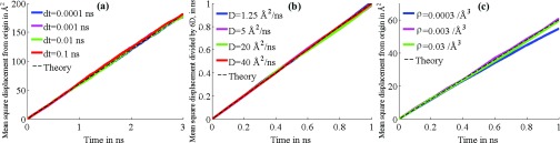
Results for series 1 tests. Except for dt = 0.0003/Å in (c), graphs in each test set are almost identical and obscure each other as a result. (a) Mean square displacement for varying time steps. (b) Mean square displacement for varying diffusion coefficients. (c) Mean square displacement for varying grid densities.

In series 2, absorptive and reflective boundary conditions were imposed: cells on the spherical shell of radius r₁ = 10 Å were assigned absorptive faces, while cells on the shell of radius r₂ = 30 Å were assigned reflective faces. Figure 3c shows the geometry of the system. Particles were initialized in cells with centers within 0.5 Å of the shell of radius r_i = 20 Å, and then allowed to diffuse until all particles had been absorbed. The particle count was tracked as a function of time and compared against the theoretical behavior, given by Eq. A26c derived in Appendix A, and found in Carslaw and Jaeger⁴⁰ (2nd ed., Eqs. (12)–(15) on p. 367).

Figure 3.

Results for series 2 tests. Graphs in each test set are almost identical and obscure each other as a result. (a) Particle number for varying time steps. (b) Particle number for varying grid densities. (c) (Top) Schematic of system used for series 2; (bottom) radial profile of grid density assumed.

In set 2A, the sample size was 10⁴ for each trial, the diffusion coefficient D = 150 Ų/ns, the grid density ρ₁ = 0.5/ų within radius 15 Å of the center and ρ₂ = 0.25/ų from 20 Å to the system boundary at 35 Å, with the value scaling down linearly between 15 Å and 20 Å; the time step was varied across values dt = 0.0002, 0.002, 0.02 ns. The results shown in Fig. 3 closely approximate the results from the analytical solutions with differences in time step size resulting in negligible differences in results on the time evolution of particle number. In set 2B, the sample size was 10⁴, D = 150 Ų/ns, dt = 0.02 ns, and grid density was varied across values {ρ₁, ρ₂} = {0.1/ų, 0.05/ų}, {0.1/ų, 0.25/ų}, {0.5/ų, 0.05/ų}, {0.5/ų, 0.25/ų}.

In a final series of trials, the system and parameters used in sets 3A and 3B were the same as those in sets 2A and 2B. However, a linear potential U(x) = α||x|| was imposed, with α = 0.2 k_BT/Å. The results for the respective sets are shown in Fig. 4 and compared with the results from the analytic solution, given by Eq. A27 in Appendix A. Again, the numerical results are accurate over the range of values of parameters tested.

Figure 4.

Results for series 3 tests. Graphs in each test set are almost identical and obscure each other as a result. (a) Particle number for varying time steps. (b) Particle number for varying grid densities.

The time step-independence of the results in Figs. 234 is not unexpected, since the solution 35 of the restricted matrix is exact. In theory, the accuracy of the MSM description decreases with a decrease in the size of the time step³² because of the implicit assumption that the equilibration time of the particle within the cell at the beginning of each time step is negligible. The implication for our model is that accuracy is independent of time step size above a certain minimum time step size, subject to other parameter values, in particular the radius of the restricted region r_restrict, which must be set large enough that the particle's movement is not significantly hindered by the artificial boundaries. The other source of inaccuracy is error due to discretization as one assumes a uniform distribution in the grid cells. This error may be detected by varying either the rate at which particles move from cell to cell or by varying the grid resolution. In this regard, the results of set 1C suggest that boundary interactions are a more significant source of discretization error than is bulk diffusion.

COMPUTATIONAL EFFICIENCY

The simulation process applied in our numerical solutions can be divided into three major phases according to computational expense: discretization of the system, calculation, and solution of the rate matrix, and Brownian motion algorithm for the diffusive displacement of particles. In the discretization phase, the most expensive task to be performed is the adaptation of cell centers, which requires updating N positions in S adaptation steps. Hence, the complexity for the first phase goes as O(N · S).

In the second phase, the bottleneck occurs during the solution of the rate matrix, more specifically during the calculation of eigenvectors and eigenvalues for the neighborhood within radius r_restrict = 2r_Δt of each cell center w_i. Given the average density ρ, the approximate number of cells within each neighborhood is $\frac{4}{3}\pi {\left(2r_{\Delta t}\right)}^3\rho =\frac{32}{3}\pi \rho {\left(6D\Delta t\right)}^{3/2}$. A modest ballpark estimate for the complexity of eigenvector expansion is O(n³). For N cells, this estimate gives O(Nρ³(DΔt)^9/2) complexity for the eigenvector expansion phase. By this estimate, we justify the algorithmic step of solving restricted matrices as opposed to solving the entire rate matrix: depending on the characteristics of the system and grid chosen, it is often the case that the O(N³) complexity of solving the entire matrix overshadows that of solving the restricted matrices.

In the final phase, given particle number M and a total simulation time t_total, the complexity is O(M · t_total/Δt).

The computationally most expensive phase is typically the second one. Fortunately, the calculations for each cell neighborhood can be performed independently of those for other neighborhoods, and, thus, are amenable to parallelization. Furthermore, eigenvector expansion algorithms themselves can sometimes be parallelized. Hence, there is much potential for the reduction of the overall computation time needed.

REALISTIC APPLICATION: ION DIFFUSION THROUGH THE MECHANOSENSITIVE CHANNEL OF SMALL CONDUCTANCE

Mechanosensitive channels of small conductance (MscS) are a class of membrane channels that are gated by membrane tension. One such channel in Eschericia coli (ecMscS) is part of the bacterium's mechanism of coping with osmotic stress. The increased tension in the membrane during osmotic stress activates ecMscS, allowing the passive efflux of cytoplasmic solutes, thereby mitigating a potentially fatal buildup of osmotic pressure.³

ecMscS, shown in Fig. 5, is a heptamer of identical subunits, which form a trans-membrane domain and a cytoplasmic domain (CD). The CD is shaped like a balloon with seven lateral openings corresponding to its sevenfold symmetry. The lateral openings are just large enough for ions, the key osmolytes in E. coli cells, to pass through. The prevalent positive ions in E. coli cells are K⁺ and Na⁺, while the main negative ion is actually the amino acid glutamate, Glu⁻.³ An additional opening exists on the end of the CD distal to the membrane, but this opening is too narrow and hydrophobic for ions to pass through.

Figure 5.

Three ecMscS channels embedded in a membrane. ecMscS is composed of seven identical subunits (each shown in a different color). ecMscS (shown in shades of green) has a transmembrane domain (faintly visible in the membrane in case of the ecMscS closest to the viewer), forming a channel that opens and closes in the presence or absence of significant osmotic pressure across the cell membrane. ecMscS also has a large extra-membrane domain pointing into the cell interior, the cytoplasm. This domain of ecMscS is called the cytoplasmic domain and is prominently visible in the figure for all three ecMscS proteins. The membrane is a bilayer of lipids; lipids are composed of head groups (shown as orange and blue spheres) and tails (shown as white lines). Ions (positive ions shown as blue spheres, negative ions as red spheres) diffuse through the bulk solvent, the cytoplasm, as seen here below the membrane. Ions enter the ecMscS cytoplasmic domains through the side openings into the domain interior and, in case of osmotic stress having induced an opening of the ecMscS trans-membrane channel, pass through the channel towards the space outside of the cell, the periplasm. The intricate geometry of the cytoplasmic domain, a roughly spherical interior connected to the cytosol through seven narrow openings, plays a determining role in the manner in which ions leave an osmotically challenged cell. The labels shown on the figure correspond to: 1. Periplasm; 2. cytoplasm; 3. membrane; 4. cytoplasmic domain of ecMscS; 5. side openings; 6. ions.

The function of the ecMscS CD is not well-understood despite its considerable size and large fraction of protein mass that goes into it. It is worth noting that CDs are a ubiquitous feature of ion channels, present in both Kv^{41, 42, 43} and Kir^{44, 45, 46} classes of potassium channels, some members of the family of voltage-gated sodium channels,⁴⁷ the sodium-potassium pump,⁴⁸ the ClC chloride channel,⁴⁹ the nicotinic acetylcholine receptor and its homologs,^{50, 51} and the family of mechanosensitive channels.^{52, 53} In most of these channels, the role of the CD has only in recent years become the subject of many investigative efforts,^{3, 54, 55, 56, 57, 58, 59, 60, 61} as the importance of the respective CDs' roles in channel function becomes more evident. In particular, CDs are believed to play a role in regulating the diffusion of ions through the pores of certain channels.

In the case of ecMscS, one postulate is that the CD plays a role in gating and in this case would necessarily undergo a large conformational change between the open and closed states of the channel.^{62, 63, 64} It has also been suggested that the CD stabilizes the structure of the channel.^{65, 66} Another postulate is that the CD acts as a molecular filter that minimizes the loss of Glu⁻ solutes.⁵³ Such a filter may also encourage the efflux of cations and anions in pairs such that the efflux is electrically neutral, so as to maintain the cellular membrane potential. More recent studies compared ecMscS with channels exhibiting a similar CD structure, namely, bacterial cyclic nucleotide-gated (bCNG) channels, MscS-Like proteins of Arabidopsis thaliana (MSL10) and Thermoanaerobacter tengcongensis MscS (TtMscS). bCNG channels display slight or no mechanosensitive gating response,⁶⁷ suggesting that the CD plays at most a limited role in channel gating; the fact that MSL10⁶⁸ and TtMscS⁶⁹ are highly anion-selective casts doubt on the view that the CD enforces current neutrality.

Previous attempts to simulate MscS function using MD and Monte Carlo methods showed high selectivity for anions.²⁴ These simulation results run counter to experimental measurements that indicate a much lower selectivity.^{70, 71, 72} Barring inaccuracies associated with the simulation method, the results of experiment and simulation may be reconciled if collective inter-ion interactions occur over time scales beyond the reach of the previous simulation methods used (∼10 μs), that compensate for the channel's bias towards anions. Apart from such interactions, the diffusive approach of the ions to the channel may also play an important role in the description of ion efflux, for example, if the time scale of the diffusive approach is longer than the time scale of passage through the channel. Simulated ion channel systems are typically not large enough to take into account the diffusive approach, which occurs over length scales of 10–100 nm. Addressing the needs for such long time and large length scales requires the simulation of ecMscS in a large box and necessitates the present method. We note that one can use a lower grid density to describe the large regions further away from the channel and a higher grid density for the channel and its vicinity.

However, since the current version of the present method treats particles independently, we cannot yet address the question of ion-ion interactions. Hence, the purpose of this section is not to obtain new results on MscS function. Instead, our simulation of ecMscS serves as a demonstration of the implementation of the method in an actual application, as well as to show that the results obtained are consistent with previous studies of the same system using the BioMOCA software and MD.²⁴ Future modifications of the presented methodology to include inter-ionic interactions will address multi-ion conduction through the ecMscS CD and membrane channel.

Setup of molecular dynamics simulation

The system is described through an all-atom MD simulation with ecMscS embedded in the center of a 320 Å × 320 Å POPC membrane patch, immersed in a waterbox of dimension 316 Å × 317 Å × 230 Å. Ions are placed in the solvent in numbers according to physiological ion strengths [K⁺], [Glu⁻], and [Cl⁻], such that the system is electrically neutral. The system is minimized and equilibrated in the presence of an electric field as described before²⁴ so as to widen the ecMscS pore relative to the opening seen in the crystal structure.⁵³ Full details of the all-atom system setup and simulation parameters are furnished in Appendix B.

PMF maps of the system for both K⁺ and Glu⁻ were extracted from a 240-ns equilibration run. For the extraction the applied electric field was removed and the backbone of ecMscS was harmonically restrained to prevent the pore from closing. The distributions of K⁺ and Glu⁻ ions were averaged over the entire course of the run. Regions where the distribution went to zero were assigned a minimal non-zero distribution value, in order to prevent singularities from occurring when taking logarithms in the next step: the logarithm of the averaged distribution map, after normalization, gives the PMF map in units of k_BT.

The diffusion coefficients of K⁺ and Glu⁻ were assumed to be constant in space. The average value of each coefficient was obtained from trajectories arising from the MD simulation described above. The trajectories were divided into 0.02 ns intervals. In each interval, the mean square displacement of each ionic species between the beginning and the end of the interval was measured. The mean square displacement values were then averaged over all intervals. Thus, the diffusion coefficient D for each ionic species was calculated from the relation ⟨Δx²(t)⟩ = 6Dt. The diffusion coefficients were found to assume the values D_K = 200 Ų/ns and D_Glu = 75 Ų/ns, which are in close agreement with the experimentally determined values^{73, 74} of $D_{\mathrm{K}}^{\mathrm{expt}}=196{\AA }^2/\mathrm{ns}$ and $D_{\mathrm{Glu}}^{\mathrm{expt}}=75{\AA }^2/\mathrm{ns}$ (both measured in bulk solvent), respectively.

A grid representing the discretized system was built, with density ρ₁ = 0.05/ų within a radius of 70 Å (large enough to encapsulate the ecMscS, as shown in Fig. 6a, such that the center of the CD coincides with the center of the grid) and ρ₂ = 0.01/ų outside of a radius of 80 Å with the center of the CD being characterized through zero radius. The density was adapted linearly with the radius between 70 Å and 80 Å. The PMF map, obtained as values on a Cartesian grid, was cubic-interpolated to assign a PMF value to each cell center. Grid cells with the maximum PMF value (shown in Fig. 6b), corresponding to regions where the ion distribution is zero, were designated as reflective boundaries. Consequently, these cells were excluded from the rate matrix calculation and solution, thus reducing the total computational cost; correspondingly, cells on the boundary of the system were assigned reflective surfaces.

Figure 6.

All-atom system simulated for the present study. (a) ecMscS (1) embedded in a membrane (2) and solvated in a waterbox (3). The highlighted circle represents a locus of 70 Å about the origin, in which a high grid density is used to model ion diffusion in detail near ecMscS. (b) Cells from the resulting grid that are associated with high PMF values and, hence, modeled through reflective barriers.

For a time step of dt = 0.002 ns, the rate and transition matrices were calculated, as outlined in Sec. 2C.

Simulation procedure and results

Particles were initialized in randomly chosen cells on the cytoplasmic side. The random selection was performed with weights proportional to the volume of each cell, so that the particles were initially uniformly distributed. The particles were then allowed to diffuse. When a particle crosses via ecMscS from the cytoplasmic side to the periplasmic side of the membrane, it is assumed to diffuse away from the membrane and, accordingly, is removed from the system. For the purpose of assessing the effect of transmembrane potential biases, we conducted the prior MD simulations with positive and negative biases, in addition to a zero bias simulation. We choose the strengths of the voltage bias following the study of Sotomayor et al.,⁷⁵ which we will use as a reference for comparison. For each voltage bias, an MD simulation was carried out to obtain the requisite PMF map. The PMF maps were each applied to the present method as described below.

The simulation procedure was repeated for six runs – two ion species, each with bias voltages 0 mV, +100 mV, −100 mV (measured from the cytoplasmic side). For each simulation, the initial particle count was 5000, and the total simulation time was 4 μs. The number of conduction events for each run is listed in Table 1. Table 2 shows the results of the present study, scaled to match the initial particle concentration and simulation time of the reference study, together with the results for two putative open conformations of ecMscS in the reference study.⁷⁵

Table 1.

Number of conduction events for each ion for different biasing voltages.

Ion	0 mV	+100 mV	−100 mV
K+	222	1992	34
Glu−	217	54	20

Table 2.

Comparison between present and reference study. Values for the present study have been scaled to account for the different initial particle concentration and simulation time in the reference study. The present study employed Glu⁻ ions, whereas the reference study employed Cl⁻ ions. The reference study employed two distinct putative open conformations of the channel. For each respective ion and bias, the results for both conformations are presented, separated by a comma.

	Present			Reference
Ion	0 mV	+100 mV	−100 mV	0 mV	+100 mV	−100 mV
K+	2	20	0	2, 5	13, 23	3, 0
Glu−	2	0	0	22, 40	6, 17	53, 72

In agreement with the reference study, there were few conduction events for K⁺ with bias voltages 0 mV and −100 mV. For Glu⁻, the numbers of events were much smaller than in the reference study where actually Cl⁻ ions were used.

DISCUSSION OF RESULTS AND FUTURE DIRECTIONS

The results for K⁺ in the present study agree with those of the reference study, while those of Glu⁻ differ significantly. The significantly lower event count for the anion is attributed to the fact that the present study employed bulky Glu⁻ ions as compared to the Cl⁻ ions employed in the reference study. Glu⁻ ions are actually the prevalent negative ions in E. coli, which is why they have been employed here. During the MD calculations, not only would the bulk diffusion coefficient of the anion be lower in the present study than in the reference one as reported⁷⁶ (the diffusion coefficient of Cl⁻ is similar to that of K⁺), but also the resulting steric exclusion in narrow regions around ecMscS results in higher potential barriers in the Glu⁻ PMF maps.

Other factors contribute to the discrepancies between the results of the present study and the reference study. An examination of the PMF maps shown in Fig. 7 reveals potential wells in the vicinity of the ecMscS structure. Ions congregating in these wells present an obstacle to other ions that would otherwise also enter the wells. However, in the absence of inter-ionic interactions, the lack of steric exclusion and local electrostatic interactions in the present version of the kinetic model allows the ions to all linger in the wells, substantially increasing the time taken to reach their designated targets. In fact, for the −100 mV bias, a well of −30 kcal/mol trapped Glu⁻ ions such that few conduction events arose (see Table 1). Such an effect had been avoided in the reference study because inter-ionic interactions were included in the respective simulations.

Figure 7.

(a) Cross-section of potential of mean force maps for K⁺ ions. (b) Cross-section of potential of mean force maps for Glu⁻ ions. The energy landscape for ions exhibit higher, more unfavorable values for positive ions inside the cytoplasmic domain and, conversely, lower, more favorable values for negative ions. Indeed, in the molecular dynamics simulations for the three bias conditions tested, anions congregated in the cytoplasmic domain and sterically hindered the passage of cations.

The absence of steric effects in the kinetic simulation illustrates the issues arising from the absence of inter-ionic interactions in simulations, especially in regions where ions come into close proximity of one another, such as in the channel interior. Adding inter-ionic interactions in a manner that is both physically sensible and computationally feasible is difficult because such interactions are modulated by environmental factors as well as by the presence of more than two particles within interaction range.

In light of the challenging nature of an account of ion-ion interactions, we propose as a first step a naive solution. One starts by identifying local regions in the system with roughly similar environments. One such region might be the interior of the ecMscS structure, namely, the interior of the pore and the CD, and a second might be everywhere outside it. For each region, one determines then the pair correlation function g(r) for the various ion pairs, K⁺ − K⁺, Glu⁻ − Glu⁻, and K⁺ − Glu⁻, from the MD trajectories used for the PMF extraction. g(r) can then be used to modulate the transition matrix probabilities of particles that move within a pre-set interaction range of each other.

Another issue of concern is the handling of diffusion coefficients. The assumption in the present study is that the diffusion coefficient for each ion species is constant throughout the system. This assumption was made for the sake of simplicity. However, one expects that the diffusion coefficient of glutamate in the crowded interior of the CD is very different from that in bulk solvent outside of the CD. The proposed remedy is to average over diffusion lengths of ions in local regions of the systems throughout the MD trajectories and from these lengths obtain the local diffusion coefficient in each grid cell.

It would also behoove us to ensure that the constant-value approximation of the diffusion coefficient, and other quantities for that matter, within each grid cell is valid. For that purpose, one could either interpolate the PMF and diffusion coefficient maps within the cell, or use a sufficiently fine grid to describe regions in which the maps vary sharply. The former would be difficult to implement within the present framework due to the complexity of the additional computation required. The latter can conceivably be a future addition to the algorithm that calculates, for each region, the grid density that resolves the local gradient of maps such that the error between the approximation and the actual quantities fall below a pre-set threshold. Since the PMF map describes the geometry of the system, such a scheme would also be a natural means of quantifying the suitability of grid density to the geometric intricacy of the system.

Since the utility of the present method relies greatly on its computational efficiency, it would be useful to consider alternative ways of solving the rate equation 18. In particular, one could consider employing a Chebyshev expansion⁷⁷ to approximate the solution

$$\mathbf{P}\left(t\right)=e^{\mathbf{R}t}.$$ (38)

Incorporating such a scheme into the solution of either the rate equation directly or of the local rate matrices one can compare the resulting efficiency with the present method.

CONCLUSION

The kinetic model of diffusion described in the present study is a feasible means of simulating diffusion in cellular systems over a wide range of length and time scales. Results from validation tests show robust agreement with analytic descriptions over time step sizes and diffusion coefficients typical of biomolecular systems. Furthermore, the method is adaptable to a wide range of scientific needs and computational capabilities, through the adjustment of simulation parameters. The method can be made more efficient through parallelization of the algorithm and is viable for both deterministic and stochastic calculations.

Algorithmic benefits of the method include accuracy that increases with time step and the restriction of calculations to a local region around each state. These benefits were brought to bear in the ecMscS example, where a simulation on the length scale of hundreds of Ångstroms and a time scale of 1 μs was run serially and completed in two days. The ecMscS example produced agreement with the reference study in the case of K⁺. The examples presented also illustrate the weaknesses of our method, which serve as pointers for future development, namely, the inclusion of dielectric effects, the use of position-dependent diffusion coefficients and the inclusion of inter-ion interactions.

APPENDIX A: ANALYTICAL AND NUMERICAL SOLUTIONS TO DESCRIBE SYSTEMS USED IN VALIDATION

Analytical solution for validation Sets 2A and 2B

Here, we provide the solution of the diffusion problem for test set 2. The solution is available from Carslaw and Jaeger⁴⁰ (2nd ed., Eqs. (12)–(15) on p. 367), but rather than explaining the terms and constants in the complex solution expression stated by these authors, we derive the solution here as an optimal means of communication to the reader not versed in diffusion theory.

The system is spherically symmetric, with particles diffusing in the space between two concentric spheres of radii r₁ and r₂, as shown in Fig. 3c. At time t = 0, particles are uniformly distributed on a spherical surface of radius r_i, with r₁ < r_i < r₂. The diffusion coefficient D is taken to be constant.

The free diffusion equation is given by

$$({\nabla }^2-D^{-1}{\partial }_t)p(\mathbf{r},t)=0.$$ (A1)

Using the ansatz

$$p(\mathbf{r},t)=e^{\omega t}{Y}_l^m(\theta ,\varphi )R\left(r\right),$$ (A2)

one obtains for the radial dependence

$$[{\partial }_r^2+\frac{2}{r}{\partial }_r-\frac{l(l+1)}{r^2}-\frac{\omega }{D}]R\left(r\right)=0.$$ (A3)

The above equation is known as the spherical Bessel equation, the solutions of which substitute into Eq. A2 to give the form

$$p(\mathbf{r},t)=\sum _{k,m,l}{e}^{\omega t}{Y}_l^m(\theta ,\varphi )(A_{kl}{j}_l\left(kr\right)+B_{kl}{n}_l\left(kr\right)),$$ (A4)

where j_l and n_l are the spherical Bessel functions, k is defined through $k^2=\frac{-\omega }{D}$ (ω is less than zero), $Y_l^m(\theta ,\varphi )$ represents a set of functions called the spherical harmonics, and A_kl and B_kl are constants.

Due to spherical symmetry, only the l = 0 term contributes to the solution, so that

$$p(\mathbf{r},t)=\sum _k{e}^{\omega \left(k\right)t}{R}_k\left(r\right),$$ (A5)

where

$$\begin{array}{c}\hfill R_k\left(r\right)=A_k{j}_0\left(kr\right)+B_k{n}_0\left(kr\right),\end{array}$$ (A6)

$$\begin{array}{c}\hfill j_0\left(kr\right)=\frac{\sin \left(kr\right)}{kr},\end{array}$$ (A7)

$$\begin{array}{c}\hfill n_0\left(kr\right)=-\frac{\cos \left(kr\right)}{kr},\end{array}$$ (A8)

and A_k and B_k are constants to be determined.

In our description, we assume Dirichlet and Neumann boundary conditions at r = r₁ and r = r₂, respectively. At r = r₁ holds

$$R_k\left(r_1\right)=0.$$ (A9)

For the convenience of calculation, a constant phase may be introduced without loss of generality

$$\begin{array}{c}\hfill \sin \left(kr\right)\to \sin \left[k(r-r_1)\right],\end{array}$$ (A10)

$$\begin{array}{c}\hfill \cos \left(kr\right)\to \cos \left[k(r-r_1)\right].\end{array}$$ (A11)

Then, Eq. A9 implies that $B_k=0\forall k\in \mathbb{R}$. Thus it holds

$$R_k\left(r\right)=A_k\frac{\sin \left[k(r-r_1)\right]}{kr}.$$ (A12)

At r = r₂, the Neumann boundary condition is assumed

$${\partial }_r{R}_k{\left(r\right)|}_{r=r_2}=0.$$ (A13)

This condition reads

$$-\frac{\sin \left[k(r_2-r_1)\right]}{k{r}_2^2}+\frac{\cos \left[k(r_2-r_1)\right]}{r_2}=0$$ (A14)

or

$$\tan \left[k(r_2-r_1)\right]=k{r}_2.$$ (A15)

The numerical solution of Eq. A15 gives a countably infinite set of values of k. For the sake of clear notation, let n index these values. Accordingly, we re-index the following terms:

$$\begin{array}{c}\hfill R_k\left(r\right)\to R_n\left(r\right),\end{array}$$ (A16)

$$\begin{array}{c}\hfill \omega \left(k\right)\to {\omega }_n,\end{array}$$ (A17)

$$\begin{array}{c}\hfill A_k\to A_n.\end{array}$$ (A18)

Defining the inner product in solution space as

$$⟨R_{n_1}|R_{n_2}⟩={\int }_{r_1}^{r_2}{r}^2{R}_{n_1}\left(r\right)R_{n_2}\left(r\right)dr,$$ (A19)

it can be verified that $\left\{R_n\right|n\in \mathbb{Z}\}$ is an orthogonal set. The normalization factor is obtained by evaluating

$$\begin{array}{c}\hfill A_n^{-2}⟨R_n|R_n⟩={\left(k_n\right)}^{-2}{\int }_{r_1}^{r_2}{\sin }^2\left[k_n(r-r_1)\right]dr\end{array}$$ (A20a)

$$\begin{array}{c}\hfill =\frac{1}{2k_n^2}(-r_1+\frac{k_n^2{r}_2^3}{1+k_n^2{r}_2^2}).\end{array}$$ (A20b)

Hence, the inner product can be explicitly written

$$⟨R_{n_1}|R_n⟩=A_n^2\frac{{\delta }_{n_1,n}}{2k_n^2}(-r_1+\frac{k_n^2{r}_2^3}{1+k_n^2{r}_2^2}).$$ (A21)

The complete solution is then

$$p(\mathbf{r},t)=\sum _n{e}^{{\omega }_{n}t}{R}_n\left(r\right),$$ (A22)

where ${\omega }_n=-k_n^{2}D$.

In the case of the assumed initial condition $p_0\left(\mathbf{r}\right)={\left(4\pi r_i^2\right)}^{-1}\delta (r-r_i)$ follows:

$$\sum _n{R}_n\left(r\right)={\left(4\pi r_i^2\right)}^{-1}\delta (r-r_i).$$ (A23)

Taking the inner product gives

$$⟨R_m|R_m⟩={\left(4\pi r_i^2\right)}^{-1}{\int }_{r_1}^{r_2}{r}^2{R}_m\left(r\right)\delta (r-r_i)dr,$$ (A24)

from which follows:

$$\begin{array}{c}\hfill A_m=A_m{\left(4\pi ⟨R_m|R_m⟩\right)}^{-1}{R}_m\left(r_i\right)\end{array}$$ (A25a)

$$\begin{array}{c}\hfill =\frac{k_m^2}{2\pi }{(-r_1+\frac{k_m^2{r}_2^3}{1+k_m^2{r}_2^2})}^{-1}\frac{\sin \left[k_m(r_i-r_1)\right]}{k_m{r}_i}.\end{array}$$ (A25b)

Finally, the expression of the number of surviving particles as a function of time is

$$\begin{array}{c}\hfill \Sigma \left(t\right)={\int }_{r_1}^{r_2}dr4\pi r^{2}p(r,t)\end{array}$$ (A26a)

$$\begin{array}{c}\hfill =4\pi {\int }_{r_1}^{r_2}dr\sum _n{A}_{n}r{e}^{-k_n^{2}Dt}\frac{\sin \left[k_n(r-r_1)\right]}{k_n}\end{array}$$ (A26b)

$$\begin{array}{c}\hfill =4\pi \sum _n{e}^{-k_n^{2}Dt}\frac{A_n{r}_1}{k_n^2}.\end{array}$$ (A26c)

Numerical mean first passage time description for validation sets 3A and 3B

In the case of a linear potential U(r) = αr, a closed-form analytic solution for the time-dependent diffusion probability does not exist. Instead, the time dependence of the probability distribution was captured for the test purpose by the mean first passage time approximation.⁷⁸ In this approximation, the normalized surviving particle count is given by

$$\Sigma \left(t\right)=e^{-t/\tau \left(r_i\right)},$$ (A27)

where τ(r_i) is the mean first passage time given by the expression

$$\tau \left(r_i\right)={\int }_{r_1}^{r_i}dr{\left(D{r}^2\right)}^{-1}{e}^{\alpha r}{\int }_r^{r_2}d{r}^{\prime }{r}^{\prime 2}{e}^{-\alpha r^{\prime }}.$$ (A28)

Here τ(r_i) is evaluated through numerical integration.

The mean passage time description through Eqs. A28, A27 is known to be a good approximation to the decay of the total probability of still unreacted particles⁷⁸ and, hence, Eqs. A28, A27 can serve as a test of the numerical scheme suggested in the present study.

APPENDIX B: SPECIFICATIONS FOR MD SIMULATION OF ecMscS SYSTEM

The structure of ecMscS, solved through x-ray crystallography,⁵³ was taken from the protein data bank (PDB 1MXM). The psfgen plugin of VMD 1.9.1⁷⁹ was used to add missing hydrogens to the structure. Asp, Glu, Lys, and Arg were modeled as charged residues. The structure was then aligned with a 320 Å × 320 Å POPC membrane patch such that the transmembrane domain was superimposed on the center region of the patch; the overlapping lipids were deleted. Subsequently, the Solvate plugin in VMD was employed to immerse the protein-embedded membrane in a waterbox of dimension 316 Å × 317 × 230 Å and the cIonize plugin of VMD was employed to place K⁺ and Cl⁻ ions in the solvent, such that the concentration of each ion was 200 mM, the physiological concentration of K⁺ in the E. coli cytosol. The physiological concentration of Cl⁻ is on the order of 10 mM,⁸⁰ while that of Glu⁻ has been reported to vary over a wide range of values.⁸¹ Hence, enough Cl⁻ ions were kept in the system to give 10 mM concentration, while the rest were mutated into Glu⁻ zwitterions. Since ecMscS has a net charge of +28e, 28 K⁺ ions were deleted to neutralize the system. Due to Glu⁻ being larger in size than Cl⁻, it was necessary to delete water molecules that overlapped with the Glu⁻ zwitterions. The final system contained 610 961 water molecules, 2997 lipids, 2307 K⁺ ions, 100 Cl⁻ ions, and 2235 Glu⁻ zwitterions. The total atom count of the system was 2 304 943.

MD simulations were run with NAMD 2.9,⁸² using the TIP3P water model,⁸³ and with the CHARMM36⁸⁴ and CMAP-corrected CHARMM22⁸⁵, ⁸⁶ force fields for lipids and non-lipids, respectively. The time step was set to 2 fs. The particle mesh-Ewald method was used to calculate long-range electrostatic forces, with a mesh density of 1/ų. Van der Waals forces were calculated with a cut-off of 12 Å and a switching function starting at 10 Å. Periodic boundary conditions were imposed in all MD runs. Temperature was held at 300 K via Langevin dynamics with a damping coefficient of 1 ps⁻¹. Pressure was held at 1 atm using the Nosé-Hoover Langevin piston method with damping time of 50 fs and period of 200 fs.

The system was minimized over 3.4 × 10⁵ steps. All atoms, except for those of the lipid tails, were fixed during the subsequent 4.6 ns equilibration to allow the lipid tails to melt. Lipid head group constraints were then released and equilibration continued for another 10 ns, to allow the membrane to form a watertight seal around the ecMscS pore. The system was then put through 10 cycles of alternating runs, the first being un-constrained equilibration with voltage 0.6 V across the membrane (measured from the cytoplasmic side), and the other runs being equilibration, with no applied voltage, and with ecMscS backbone atoms being harmonically constrained with spring constant 2 kcal/mol/Ų to their last positions in the previous run. The runs with applied voltage induced widening of the ecMscS pore,²⁴ while the runs with constraints on the ecMscS backbone allowed the membrane to relax back to a stable state so that the strong voltage did not break up the membrane before the ecMscS pore widened. The resulting structure was used for the production run, during which protein backbone atoms were again put under harmonic restraint with spring constant 2 kcal/mol/Ų, in order to maintain the widened pore width in the absence of an applied voltage.

MD runs for sampling the PMF and other properties were carried out for 240 ns, ensuring adequate sampling as shown in the plot of the convergence metric used in Fig. 8. The convergence metric is defined as the root mean square deviation of the potential map at 20-ns intervals from the final map during the run. Since the interior of ecMscS is the least accessible, and hence the least sampled, region of the system, we confine the convergence metric calculation to a box which just encloses the protein.

Figure 8.

Root mean square deviation of the sampled PMF from the final map in a 84Å × 84 × 120 Å box enclosing the ecMscS channel.

References

- Peters R., Brünger A., and Schulten K., Proc. Natl. Acad. Sci. U.S.A. 78, 962 (1981). 10.1073/pnas.78.2.962 [DOI] [PMC free article] [PubMed] [Google Scholar]
- Lamm G. and Schulten K., J. Chem. Phys. 75, 365 (1981). 10.1063/1.441789 [DOI] [Google Scholar]
- Gamini R., Sotomayor M., Chipot C., and Schulten K., Biophys. J. 101, 80 (2011). 10.1016/j.bpj.2011.05.042 [DOI] [PMC free article] [PubMed] [Google Scholar]
- Berg H. C. and Purcell E. M., Biophys. J. 20, 193 (1977). 10.1016/S0006-3495(77)85544-6 [DOI] [PMC free article] [PubMed] [Google Scholar]
- Shoup D. and Szabo A., Biophys. J. 40, 33 (1982). 10.1016/S0006-3495(82)84455-X [DOI] [PMC free article] [PubMed] [Google Scholar]
- Sharp K., Fine R., Schulten K., and Honig B., Phys. Chem. 91, 3624 (1987). 10.1021/j100297a032 [DOI] [Google Scholar]
- Zwanzig R. and Szabo A., Biophys. J. 60, 671 (1991). 10.1016/S0006-3495(91)82096-3 [DOI] [PMC free article] [PubMed] [Google Scholar]
- Gabdoulline R. R. and Wade R. C., Curr. Opin. Struct. Biol. 12, 204 (2002). 10.1016/S0959-440X(02)00311-1 [DOI] [PubMed] [Google Scholar]
- Atri A., Amundson J., Clapham D., and Sneyd J., Biophys. J. 65, 1727 (1993). 10.1016/S0006-3495(93)81191-3 [DOI] [PMC free article] [PubMed] [Google Scholar]
- Elf J., Dončić A., and Ehrenberg M., Proc. SPIE 5110, 114 (2003). 10.1117/12.497009 [DOI] [Google Scholar]
- Chiam K.-H., Tan C. M., Bhargava V., and Rajagopal G., Phys. Rev. E 74, 051910 (2006). 10.1103/PhysRevE.74.051910 [DOI] [PubMed] [Google Scholar]
- Camilli A. and Bassler B. L., Science 311, 1113 (2006). 10.1126/science.1121357 [DOI] [PMC free article] [PubMed] [Google Scholar]
- Sneyd J., Wetton B. T., Charles A. C., and Sanderson M. J., Am. J. Physiol.: Cell Physiol. 268, C1537 (1995). [DOI] [PubMed] [Google Scholar]
- Shvartsman S. Y., Wiley H. S., Deen W. M., and Lauffenburger D. A., Biophys. J. 81, 1854 (2001). 10.1016/S0006-3495(01)75837-7 [DOI] [PMC free article] [PubMed] [Google Scholar]
- Nadler W. and Schulten K., J. Chem. Phys. 82, 151 (1985). 10.1063/1.448788 [DOI] [Google Scholar]
- Andrews S. S., Addy N. J., Brent R., and Arkin A. P., PLOS Comput. Biol. 6, e1000705 (2010). 10.1371/journal.pcbi.1000705 [DOI] [PMC free article] [PubMed] [Google Scholar]
- Stiles J. R. and Bartol T. M., Computational Neuroscience: Realistic Modeling for Experimentalists, edited by Schutter E. D. (CRC Press, 2001), pp. 87–127. [Google Scholar]
- Cowan A. E., Moraru I. I., Schaff J. C., Slepchenko B. M., and Loew L. M., Methods Cell Biol. 110, 195 (2012). 10.1016/B978-0-12-388403-9.00008-4 [DOI] [PMC free article] [PubMed] [Google Scholar]
- Popov A. V. and Agmon N., J. Chem. Phys. 115, 8921 (2001). 10.1063/1.1412609 [DOI] [Google Scholar]
- van Zon J. S. and ten Wolde P. R., J. Chem. Phys. 123, 234910 (2005). 10.1063/1.2137716 [DOI] [PubMed] [Google Scholar]
- van Zon J. S. and ten Wolde P. R., Phys. Rev. Lett. 94, 128103 (2005). 10.1103/PhysRevLett.94.128103 [DOI] [PubMed] [Google Scholar]
- Compoint M., Picaud F., Ramseyer C., and Giradet C., J. Chem. Phys. 122, 134707 (2005). 10.1063/1.1869413 [DOI] [PubMed] [Google Scholar]
- Allen T. W., Andersen O. S., and Roux B., Biophys. J. 90, 3447 (2006). 10.1529/biophysj.105.077073 [DOI] [PMC free article] [PubMed] [Google Scholar]
- Sotomayor M., Vasquez V., Perozo E., and Schulten K., Biophys. J. 92, 886 (2007). 10.1529/biophysj.106.095232 [DOI] [PMC free article] [PubMed] [Google Scholar]
- Elber R., Curr. Opin. Struct. Biol. 15, 151 (2005). 10.1016/j.sbi.2005.02.004 [DOI] [PubMed] [Google Scholar]
- Ermak D. L., J. Chem. Phys. 62, 4189 (1975). 10.1063/1.430300 [DOI] [Google Scholar]
- McGuffee S. R. and Elcock A. H., J. Am. Chem. Soc. 128, 12098 (2006). 10.1021/ja0614058 [DOI] [PubMed] [Google Scholar]
- Frembgen-Kesner T. and Elcock A. H., J. Chem. Theory Comput. 5, 242 (2009). 10.1021/ct800499p [DOI] [PubMed] [Google Scholar]
- Ando T. and Skolnick J., Proc. Natl. Acad. Sci. U.S.A. 107, 18457 (2010). 10.1073/pnas.1011354107 [DOI] [PMC free article] [PubMed] [Google Scholar]
- van der Straaten T., Kathawala G., and Ravaioli U., J. Comput. Electron. 2, 231 (2003). 10.1023/B:JCEL.0000011430.99984.cd [DOI] [Google Scholar]
- Bauler P., Huber G. A., and McCammon J. A., J. Chem. Phys. 136, 164107 (2012). 10.1063/1.4704808 [DOI] [PMC free article] [PubMed] [Google Scholar]
- Prinz J.-H., Wu H., Sarich M., Keller B., Senne M., Held M., Chodera J. D., Schütte C., and Noé F., J. Chem. Phys. 134, 174105 (2011). 10.1063/1.3565032 [DOI] [PubMed] [Google Scholar]
- MATLAB, version 7.10.0 (R2010a), The MathWorks Inc., Natick, MA, 2010.
- Ritter H., Martinetz T., and Schulten K., Neural Computation and Self-Organizing Maps: An Introduction, revised English ed. (Addison-Wesley, New York, 1992). [Google Scholar]
- Martinetz T. M., Berkovich S. G., and Schulten K., IEEE Trans. Neural. Netw. 4, 558 (1993). 10.1109/72.238311 [DOI] [PubMed] [Google Scholar]
- Martinetz T. and Schulten K., Neural Networks 7, 507 (1994). 10.1016/0893-6080(94)90109-0 [DOI] [Google Scholar]
- Du Q., Faber V., and Gunzburger M., SIAM Rev. 41, 637 (1999). 10.1137/S0036144599352836 [DOI] [Google Scholar]
- Gumbart J. C., Teo I., Roux B., and Schulten K., J. Am. Chem. Soc. 135, 2291 (2013). 10.1021/ja310777k [DOI] [PMC free article] [PubMed] [Google Scholar]
- Madura J., Briggs J., Wade R., Davis M., Luty B., Illin A., Antosiewicz J., Gilson M., Bagheri B., Scott L., and McCammon J. A., Comput. Phys. Commun. 91, 57 (1995). 10.1016/0010-4655(95)00043-F [DOI] [Google Scholar]
- Carslaw H. S. and Jaeger J. C., Conduction of Heat in Solids (Oxford University Press, London, 1959), pp. 367–368. [Google Scholar]
- Tu L. W., Santarelli V., and Deutsch C., Biophys. J. 68, 147 (1995). 10.1016/S0006-3495(95)80169-4 [DOI] [PMC free article] [PubMed] [Google Scholar]
- Jiang Y., Lee A., Chen J., Ruta V., Cadene M., Chait B. T., and MacKinnon R., Nature (London) 423, 33 (2003). 10.1038/nature01580 [DOI] [PubMed] [Google Scholar]
- Long S. B., Campbell E. B., and MacKinnon R., Science 309, 897 (2005). 10.1126/science.1116269 [DOI] [PubMed] [Google Scholar]
- Kuo A., Gulbis J. M., Antcliff J. F., Rahman T., Lowe E. D., Zimmer J., Cuthbertson J., Ashcroft F. M., Ezaki T., and Doyle D. A., Science 300, 1922 (2003). 10.1126/science.1085028 [DOI] [PubMed] [Google Scholar]
- Tao X., Avalos J. L., Chen J., and MacKinnon R., Science 326, 1668 (2009). 10.1126/science.1180310 [DOI] [PMC free article] [PubMed] [Google Scholar]
- Uysal S., Vásquez V., Tereshko V., Esaki K., Fellouse F. A., Sidhu S. D., Koide S., Perozo E., and Kossiakoff A., Proc. Natl. Acad. Sci. U.S.A. 106, 6644 (2009). 10.1073/pnas.0810663106 [DOI] [PMC free article] [PubMed] [Google Scholar]
- Yu F. H. and Catterall W. A., Genome Biol. 4, 207 (2003). 10.1186/gb-2003-4-3-207 [DOI] [PMC free article] [PubMed] [Google Scholar]
- Shinoda T., Ogawa H., Cornelius F., and Toyoshima C., Nat. Lett. 459, 446 (2009). 10.1038/nature07939 [DOI] [PubMed] [Google Scholar]
- Dutzler R., Campbell E. B., Cadene M., Chait B. T., and MacKinnon R., Nature (London) 415, 287 (2002). 10.1038/415287a [DOI] [PubMed] [Google Scholar]
- Karlin A., Nat. Rev. Neurosci. 3, 102 (2002). 10.1038/nrn731 [DOI] [PubMed] [Google Scholar]
- Celie P. H., Kasheverov I. E., Mordvintsev D. Y., Hogg R. C., van Nierop P., van Elk R., van Rossum-Fikkert S. E., Zhmak M. N., Bertrand D., Tsetlin V., Sixma T. K., and Smit A. B., Nat. Struct. Mol. Biol. 12, 582 (2005). 10.1038/nsmb951 [DOI] [PubMed] [Google Scholar]
- Chang G., Spencer R. H., Lee A. T., Barclay M. T., and Rees D. C., Science 282, 2220 (1998). 10.1126/science.282.5397.2220 [DOI] [PubMed] [Google Scholar]
- Bass R. B., Strop P., Barclay M., and Rees D. C., Science 298, 1582 (2002). 10.1126/science.1077945 [DOI] [PubMed] [Google Scholar]
- Pegan S., Arrabit C., Zhou W., Kwiatkowski W., Collins A., Slesinger P. A., and Choe S., Nat. Neurosci. 8, 279 (2005). 10.1038/nn1411 [DOI] [PubMed] [Google Scholar]
- Han W., Nattel S., Noguchi T., and Shrier A., J. Biol. Chem. 281, 27134 (2006). 10.1074/jbc.M604843200 [DOI] [PubMed] [Google Scholar]
- Schack V. R., Morth J. P., Toustrup-Jensen M. S., Anthonisen A. N., Nissen P., Andersen J. P., and Vilsen B., J. Biol. Chem. 283, 27982 (2008). 10.1074/jbc.M803506200 [DOI] [PubMed] [Google Scholar]
- Potet F., Chagot B., Anghelescu M., Viswanathan P. C., Stepanovic S. Z., Kupershmidt S., Chazin W. J., and Balser J. R., J. Biol. Chem. 284, 8846 (2009). 10.1074/jbc.M806871200 [DOI] [PMC free article] [PubMed] [Google Scholar]
- Wray D., Eur. Biophys. J. 38, 285 (2009). 10.1007/s00249-008-0354-4 [DOI] [PubMed] [Google Scholar]
- Sharkey L. M., Cheng X., Drews V., Buchner D. A., Jones J. M., Justice M. J., Waxman S. G., Dib-Hajj S. D., and Meisler M. H., J. Neurosci. 29, 2733 (2009). 10.1523/JNEUROSCI.6026-08.2009 [DOI] [PMC free article] [PubMed] [Google Scholar]
- Hirano M., Takeuchi Y., Aoki T., Yanagida T., and Ide T., J. Biol. Chem. 285, 3777 (2010). 10.1074/jbc.M109.084368 [DOI] [PMC free article] [PubMed] [Google Scholar]
- Jin M. and Lu P., Neural Regen. Res. 6, 553 (2011). [Google Scholar]
- Edwards M. D., Booth I. R., and Miller S., Curr. Opin. Microbiol. 7, 163 (2004). 10.1016/j.mib.2004.02.006 [DOI] [PubMed] [Google Scholar]
- Koprowski P. and Kubalski A., J. Biol. Chem. 278, 11237 (2003). 10.1074/jbc.M212073200 [DOI] [PubMed] [Google Scholar]
- Grajkowskim W., Kubalski A., and Koprowski P., Biophys. J. 88, 3050 (2005). 10.1529/biophysj.104.053546 [DOI] [PMC free article] [PubMed] [Google Scholar]
- Miller S., Bartlett W., Chandrasekaran S., Simpson S., Edwards M., and Booth I. R., EMBO J. 22, 36 (2003). 10.1093/emboj/cdg011 [DOI] [PMC free article] [PubMed] [Google Scholar]
- Schumann U., Edwards M., Li C., and Booth I. R., FEBS Lett. 572, 233 (2004). 10.1016/j.febslet.2004.07.045 [DOI] [PubMed] [Google Scholar]
- Malcolm H. R., Heo Y. Y., Caldwell D. B., McConnell J. K., Hawkins J. F., Guayasamin R. C., Elmore D. E., and Maurer J. A., Eur. Biophys. J. 41, 1003 (2012). 10.1007/s00249-012-0855-z [DOI] [PubMed] [Google Scholar]
- Maksaev G. and Haswell E. S., Proc. Natl. Acad. Sci. U.S.A. 109, 19015 (2012). 10.1073/pnas.1213931109 [DOI] [PMC free article] [PubMed] [Google Scholar]
- Zhang X., Wang J., Feng Y., Ge J., Li W., Sun W., Iscla I., Yu J., Blount P., Li Y., and Yang M., Proc. Natl. Acad. Sci. U.S.A. 109, 18180 (2012). 10.1073/pnas.1207977109 [DOI] [PMC free article] [PubMed] [Google Scholar]
- Martinac B., Buechner M., Delcour A. H., Adler J., and Kung C., Proc. Natl. Acad. Sci. U.S.A. 84, 2297 (1987). 10.1073/pnas.84.8.2297 [DOI] [PMC free article] [PubMed] [Google Scholar]
- Sukharev S., Biophys. J. 83, 290 (2002). 10.1016/S0006-3495(02)75169-2 [DOI] [PMC free article] [PubMed] [Google Scholar]
- Akitake B., Anishkin A., and Sukharev S., J. Gen. Physiol. 125, 143 (2005). 10.1085/jgp.200409198 [DOI] [PMC free article] [PubMed] [Google Scholar]
- Cussler E. L., Diffusion: Mass Transfer in Fluid Systems (Cambridge University Press, 1997). [Google Scholar]
- Longsworth L. G., J. Am. Chem. Soc. 75, 5705 (1953). 10.1021/ja01118a065 [DOI] [Google Scholar]
- Sotomayor M., van der Straaten T. A., Ravaioli U., and Schulten K., Biophys. J. 90, 3496 (2006). 10.1529/biophysj.105.080069 [DOI] [PMC free article] [PubMed] [Google Scholar]
- Li Y.-H. and Gregory S., Geochim. Cosmochim. Acta 38, 703 (1974). 10.1016/0016-7037(74)90145-8 [DOI] [Google Scholar]
- Tal-Ezer H. and Kosloff R., J. Chem. Phys. 81, 3967 (1984). 10.1063/1.448136 [DOI] [Google Scholar]
- Szabo A., Schulten K., and Schulten Z., J. Chem. Phys. 72, 4350 (1980). 10.1063/1.439715 [DOI] [Google Scholar]
- Humphrey W., Dalke A., and Schulten K., J. Mol. Graphics 14, 33 (1996). 10.1016/0263-7855(96)00018-5 [DOI] [PubMed] [Google Scholar]
- Schultz S. G., Wilson N. L., and Epstein W., J. Gen. Physiol. 46, 159 (1962). 10.1085/jgp.46.1.159 [DOI] [PMC free article] [PubMed] [Google Scholar]
- Ogahara T., Ohno M., Takayama M., Igarashi K., and Kobayashi H., J. Bacteriol. 177, 5987 (1995). [DOI] [PMC free article] [PubMed] [Google Scholar]
- Phillips J. C., Braun R., Wang W., Gumbart J., Tajkhorshid E., Villa E., Chipot C., Skeel R. D., Kale L., and Schulten K., J. Comput. Chem. 26, 1781 (2005). 10.1002/jcc.20289 [DOI] [PMC free article] [PubMed] [Google Scholar]
- Jorgensen W. L., Chandrasekhar J., Madura J. D., Impey R. W., and Klein M. L., J. Chem. Phys. 79, 926 (1983). 10.1063/1.445869 [DOI] [Google Scholar]
- Klauda J. B., Venable R. M., Freites J. A., O'Connor J. W., Tobias D. J., Mondragon-Ramirez C., Vorobyov I., A. D.MacKerellJr., and Pastor R. W., J. Phys. Chem. B 114, 7830 (2010). 10.1021/jp101759q [DOI] [PMC free article] [PubMed] [Google Scholar]
- A. D.MacKerellJr., Bashford D., Bellott M., Dunbrack J. R. L., Evanseck J., Field M. J., Fischer S., Gao J., Guo H., Ha S., Joseph D., Kuchnir L., Kuczera K., Lau F. T. K., Mattos C., Michnick S., Ngo T., Nguyen D. T., Prodhom B., Roux B., Schlenkrich M., Smith J., Stote R., Straub J., Watanabe M., Wiorkiewicz-Kuczera J., Yin D., and Karplus M., FASEB J. 6, A143 (1992). [Google Scholar]
- A. D.MacKerellJr., Bashford D., Bellott M., R. L.DunbrackJr., Evanseck J. D., Field M. J., Fischer S., Gao J., Guo H., Ha S., Joseph D., Kuchnir L., Kuczera K., Lau F. T. K., Mattos C., Michnick S., Ngo T., Nguyen D. T., Prodhom B., Reiher I. W. E., Roux B., Schlenkrich M., Smith J., Stote R., Straub J., Watanabe M., Wiorkiewicz-Kuczera J., Yin D., and Karplus M., J. Phys. Chem. B 102, 3586 (1998). 10.1021/jp973084f [DOI] [PubMed] [Google Scholar]