Abstract
Distance constraints, in principle, can be employed to determine information about the location of probes within a three-dimensional volume. Traditional methods for locating probes from distance constraints involve optimization of scoring functions that measure how well the probe location fits the distance data, exploring only a small subset of the scoring function landscape in the process. These methods are not guaranteed to find the global optimum and provide no means to relate the identified optimum to all other optima in scoring space. Here, we introduce a method for the location of probes from distance information that is based on probability calculus. This method allows exploration of the entire scoring space by directly combining probability functions representing the distance data and information about attachment sites. The approach is guaranteed to identify the global optimum and enables the derivation of confidence intervals for the probe location as well as statistical quantification of ambiguities. We apply the method to determine the location of a fluorescence probe using distances derived by FRET and show that the resulting location matches that independently derived by electron microscopy.
Keywords: FRET, electron microscopy, probability function, distance data
Introduction
The multi-dimensional scoring-function landscapes encountered in structural biology tend to be rugged and complex (Frauenfelder et al., 1991; Frauenfelder and Leeson, 1998). As a consequence, simple optimization algorithms tend to get trapped in local minima, unable to locate the globally optimal solution. A multitude of search strategies such as, for example, simulated annealing (Kirkpatrick et al., 1983) or genetic algorithms (Holland, 1975) have been developed over the years in order to overcome this problem and these types of methods have been adapted to a large variety of optimization problems in structural biology (see for example Brünger et al., 2011; Webb et al., 2011; Das and Baker, 2008; Chacón et al., 1998; Brünger et al., 1998). Though superior to simple direct optimization in that they can escape local minima, these methods are neither guaranteed to identify the global optimum nor do they provide simple ways to put the found optimum into the context to other existing optima because only a small sub-set of the global scoring landscape is sampled. In contrast, if the scoring landscape can be explored in its entirety, not only the global optimum can be identified without ambiguity, it can also be related to the rest of the scoring landscape so that confidence intervals and significant levels can be obtained. It is then possible, for example, to determine whether the global optimum is actually significantly better at some desired confidence level than the second-best local optimum or whether the second-best optimum needs to be considered a viable alternative solution at that confidence level.
Recently, methods for a more complete evaluation of scoring function space based on probability theory and Bayesian inference have been introduced in the context of structure determination by NMR (Rieping et al., 2005) or with sparse data (Habeck, 2011). Bayesian inference incorporates prior information and accounts for ambiguities through probability distributions and is especially useful when the observable to parameter ratio is low and the data is insufficient to determine the parameters unambiguously. Here, we consider the location determination of a probe from distance constraints and known attachment sites. We propose a method based on probability calculus that allows exploration of the entire scoring function space by directly combining probability functions representing the data without the construction of a likelihood function as is required for Bayesian inference.
Methodology
In order to use probability calculus, we first need to convert the experimental information into adequate probability functions p(x) with
| (1) |
and
| (2) |
where the integral extends over the entire range of x, usually taken as −∞ to ∞. In the current context, x is a three-dimensional coordinate [x1,x2,x3].
In the context of location determination from distance constraints we use two types of probability functions: (i) Functions that describe the location of a known entity, for example the attachment site of a GFP label on a macromolecule or the location of the label itself and (ii) functions that describe the distance between two entities such as distances derived from fluorescence resonance energy transfer (FRET) between two fluorophores. Both these functions are continuous in nature, justifying the use of probability functions for continuous variables.
Once the location and distance information is converted into probability functions, probability calculus can be invoked to combine the information (Kolmogorov 1950). For independent information defined in the same coordinate frame, probabilities need to be point-wise multiplied at every x:
| (3) |
For independent information that has to be combined such as finding the probability of a distance sphere pj(y) at every point in space with probability pi(x), we are seeking the probability of the sum of two independent variables and a convolution operation needs to be performed:
| (4) |
where * denotes convolution. The convolution theorem states that a convolution between two functions is equivalent to the reverse Fourier transform of the product of their Fourier transforms:
| (5) |
For example, in a typical application where FRET between several labels is used to determine the location of a probe, location information from two different label pairs would be defined in the same coordinate frame and the combined probability can be constructed by simply multiplying the probability functions describing the location information of each label pair voxel by voxel in real space. In case of distance information between two labels and information about the attachment site of one of the labels, the probability functions describing these two information sources need to be convoluted.
While distance and location parameters are continuous variables and thus continuous probability functions need to be used, it is advantageous for practical purpose to define those continuous functions on a discreet grid. In particular this strategy allows the use of sums instead of integrals so that, for example, equation 2 simplifies to
| (6) |
where x is summed over all possible values. The choice of the grid size should be fine enough to account for the ruggedness of the scoring landscape so the global optimum can be determined accurately.
Practical Recipe
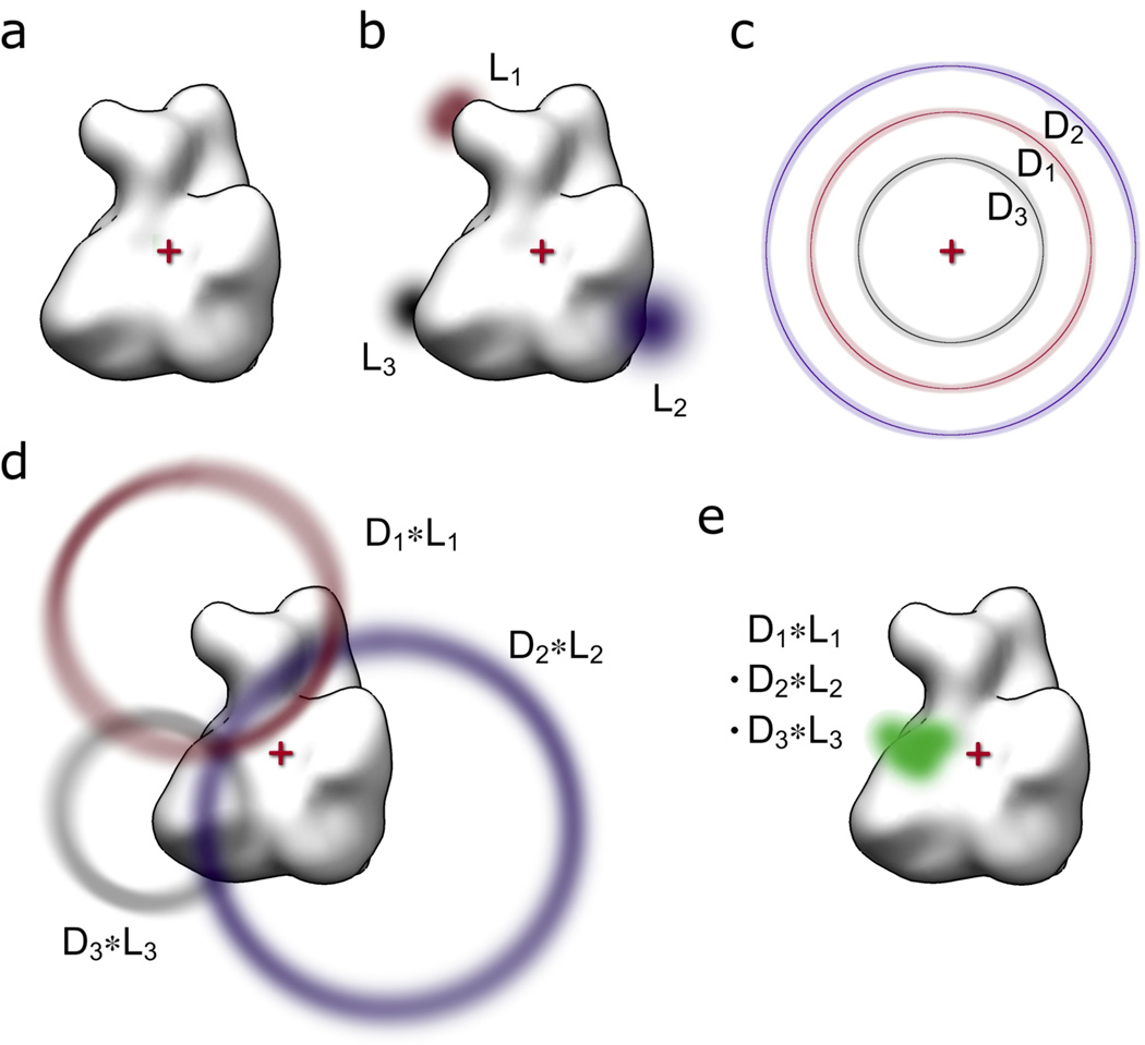
The rules described above give rise to a simple and general practical recipe for obtaining probabilities of label locations in respect to macromolecules in the presence of distance information (see also Fig 1):
Define the common coordinate system. This will usually be connected to structural information about a macromolecular assembly, for example the coordinate system where the density of an electron microscopy (EM) reconstruction is defined.
Define the bounding box. This step will provide a convenient way for normalizing all probabilities and should be large enough to contain all possible probability values appreciably larger than zero so that ∫p(x) dx = 1 inside the bounding box and ∫p(x) dx = 1 from −∞ to +∞ (equation 2) are equivalent for practical purposes. It is convenient to define the origin of the coordinate system at the bounding box center.
Define grid size for calculations. This will define how the continuous probability function is discretized. The grid size should be small enough to capture the ruggedness of the probability landscapes faithfully. Normalization is then easily achieved for each probability function by enforcing Σp(x) = 1 (equation 6), summing over all x in the bounding box.
Construct probability functions for known label locations in respect to coordinate system within bounding box. This should incorporate all anticipated uncertainties such as those coming from flexible linkers or from docking of atomic structures into lower resolution densities or envelopes. Also this step depends very heavily on the type of information available. It could be as simple as taking the coordinate of a known label location in a crystal structure, using its B-factor to get a Gaussian probability function. Some more involved cases will be presented in the application example.
Construct probability functions for distances between entities (i.e. labels) inside of bounding box, centered at origin. How this is exactly achieved will depend strongly on the method employed for determining the distances. For simple, relatively rigid cross-linkers, a Gaussian approximation would suffice, accounting for limited flexibility. A strategy for FRET distances is described in the application example.
Convolute distance probability functions and attachment-site location probabilities that refer to a single constraint (equation 2). This operation will yield the combined probability function of a single constraint in the macromolecular coordinate frame. In practical terms this is achieved by taking the reverse FFT of the product of the individual FFTs (equation 5).
Multiply all probability functions that are defined in the common coordinate system and that refer to independent constraints (equation 3).
Figure 1. Schematic overview of methodology.
(a) The common coordinate system is defined with the origin (red cross) set to the center of the macromolecular structure (white surface representation). (b) The probability functions for the locations of attachment points (L1, L2, L3) are derived in the common coordinate system. (c) The experimental distance constraints are mapped onto spheres centered at the origin to derive the corresponding probability functions (D1, D2, D3). (d) The distance and location probability functions are convoluted (LN * DN) to derive the probe location probability functions for each location/distance pair. (e) All location/distance pair probability functions are multiplied voxel-wise to derive the final probability function for the probe location (green).
The end result of this procedure gives the probability distribution of the a priori unknown location of the fluorescence probe given all the information at hand about the distances, the known label locations and their uncertainties.
Test calculations
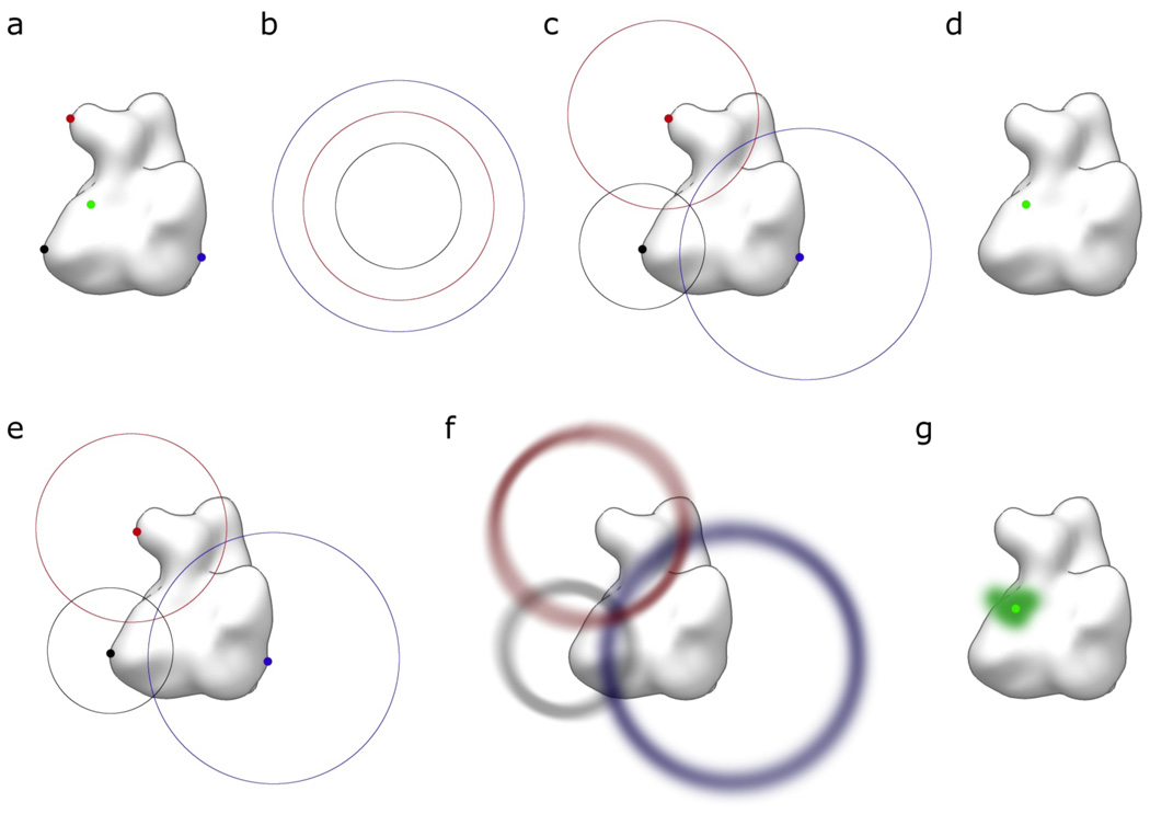
To test the procedure and demonstrate its application, we designed a simulated, two-dimensional (2D) system with known attachment-site and probe locations (Fig. 2a) as well as known distance constraints (Fig. 2b). The probability function of an attachment-site location (step 4), in case of exact knowledge in 2D, becomes a delta function (one at the location, zero everywhere else) at the respective location. The distance probability functions (step 5) become exact circles with probability zero off the circle and ∫p(x) dx = 1 running over all x on the circle (normalization condition, equation 2). To obtain the probability density of the probe location for each distance constraint/location pair, the respective probability distributions need to be convoluted (step 6, equations 4 and 5). Convolution with a delta function simply shifts the convoluted probability function to be centered at the location of the delta function (Fig. 2c). The final step is the combination of the probability functions of the location/distance pairs, which is achieved by point-by-point multiplication of the probability functions (step 7).
Figure 2. Test calculations.
(a) All attachment sites (red, blue, and black dots) as well as the probe llocation (green dot) are known exactly in respect to the macromolecule (white surface representation). (b) All distances are known exactly. (c) Convolution of the circles with the respective location delta functions shifts the circles to be centered at their respective attachment site location. Because the probability is zero for all locations off the circles, only the intersection of all three circles has non-zero probability when the circle probability functions are multiplied. (d) The final combined probe location probability function is a delta function at the known probe location. (e) If one of the contributing parameters is incorrect, the final combined probe location probability function is zero everywhere because the circles do not intersect. (f) If uncertainties are incorporated into the probability functions, overlap of non-zero probabilities is observed. (g) The final combined probe probability function encases the correct location of the probe.
Because only points on the circles have non-zero probability, the only point that has non-zero probability in the combined probability function is the intersection of the three circles. Through normalization using equation 2, this becomes a delta function at the known location of the probe (Fig. 2d). This example demonstrates that, in the limiting case of exactly known distances and locations, the method represented here arrives at the expected result. Interestingly, if only one of the parameters is incorrect but assumed to be correct (exact circles and delta functions), the circles will not all intersect in the same place and the probability function for the probe will becomes zero everywhere (Fig. 2e): the exact location can not be retrieved if parameters are estimated incorrectly. Only if uncertainties are explicitly modeled and included into the probability functions (Fig. 2f), becomes the combined probability function non-zero near the point where the three circles would meet. Furthermore, this combined probability function covers the correct location of the probe (Fig. 2g).
Application Example
To demonstrate the utility of the method and how to apply it in a practical setting, we describe in the following paragraphs how it was used to retrieve the location of a nucleation promoting factor fragment bound to the seven-subunit Arp2/3 complex using FRET derived distances. In the presence of nucleation promoting factors (NPFs), actin filaments and actin monomers, Arp2/3 complex mediates the formation of branched actin networks, thought to be necessary to exert force at the leading edge of motile cells (Pollard and Borisy, 2003). While the crystal structure of the inactive complex (Robinson et al., 2001) and an EM-derived low-resolution structure of Arp2/3 complex in the branch junction (Rouiller et al., 2008) are known, little information on the Arp2/3 conformation with bound NPFs was available until recently. We used electron microscopy and statistics-based computational density docking (Volkmann and Hanein, 1999) to derive the conformation of Arp2/3 complex in the presence of various NPFs (Xu et al., 2011). FRET pairs between GFPs at the C-termini of Arp2/3 subunits Arp2, Arp3, ARPC1 and ARPC3 respectively (Egile et al., 2005) and Texas red at the A and C ends of a Scar NPF CA fragment bound to the complex were obtained also obtained and processed with the described method to retrieve the location of CA in relation to Arp2/3 complex.
We defined the coordinate system with the origin at the center of the Arp2/3 EM density (step 1). The bounding box size BS (step 2) was derived from the maximal radius of the Arp2/3 structure RM from the origin and the maximum likely distance of all fluorescence pairs DF by BS = 2RM + 4DF. This size ensures that the probability functions themselves and any possible combined location/distance pair probability function are essentially completely contained in the bounding box so that normalization can be achieved by ensuring Σp(x) = 1 (equation 6). The grid size for discretization was chosen to be 0.1 nm (step 3). The probability functions for the attachment sites of the GFPs (step 4) were constructed by a combination of experimental data, structural modeling, and considerations about the linker flexibility.
Derivation of Attachment Site Probability Function from Experimental Data
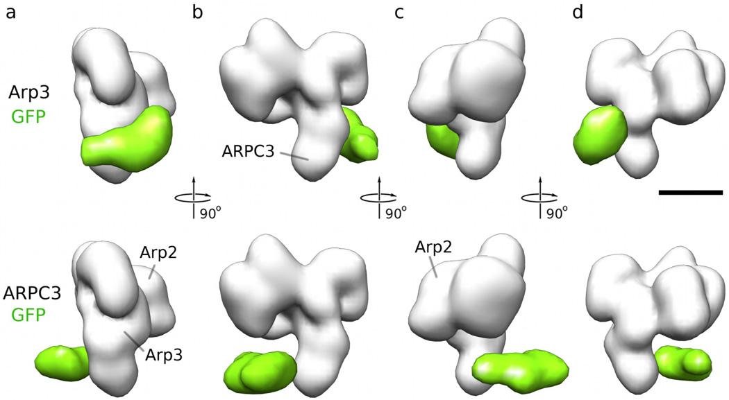
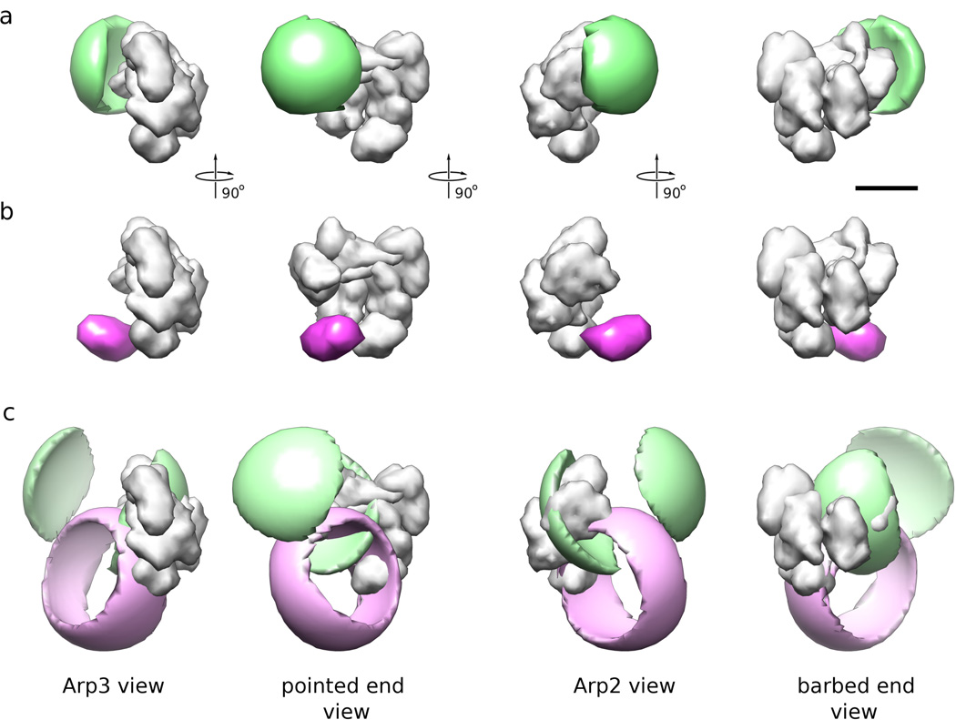
We obtained electron microscopy density maps of Arp2/3 complex with all four GFP labels at ~2 nm resolution. Only the GFPs attached to Arp3 and ARPC3 are visible in the difference maps between reconstructions from labeled and unlabeled Arp2/3 complex (Fig. 3), the other two GFPs did not produce a consistent, statistically significant density difference, most likely owing to a higher degree of mobility. To derive an approximation of the probability function, we used the following strategy: for each grid point x in the respective GFP difference map, we determined the maximum correlation coefficient cM(x), subject to rotation of the GFP density, between the difference map and a 2-nm resolution density map calculated from a GFP molecule centered at x. The probability pGFP(x) of the GPF center to be located at a specific location should then be proportional to cM(x). Note that, unless the fluorophore is spherically symmetric, this procedure is different from a simple conversion of a cross-correlation function because it includes rotational optimization at every grid location. To convert the correlation values cM(x) into probabilities pGFP(x), we only need to divide the correlation values by ΣcM(x) over all x in the bounding box so that ΣpGFP(x) = 1 (equation 6).
Figure 3. Reconstructions of Arp2/3 complex with GFP attached to the C-terminus of Arp3 (top row) and with GFP attached to ARPC3 (bottom row).
(a) Difference maps (green) calculated from the reconstruction of GFP-bound Arp2/3 complex minus the reconstruction of control Arp2/3 complex (shown for reference in white). This view is referred to as Arp3 view (b) Same as (a) turned by 90 degrees around the vertical axis of the paper plane. This view is towards the ‘barbed end’ of Arp2 and Arp3. (c) View turned by 90 degrees around the vertical axis of the paper plane from (b). This view is referred to as Arp2 view. (d) View turned by 90 degrees around the vertical axis of the paper plane from (c). This view is towards the ‘pointed end’ of Arp2 and Arp3. The size of the bar is 5 nm.
This probability function can be further refined by ensuring (i) that the center of GFP can not be closer to the surface of the Arp2/3 complex than the closest possible approach between the two and (ii) that GFP can not be further away than the covalent linker between the respective C-terminus and the GFP allows. Both these information sources contain their own uncertainties that can be derived from the confidence intervals obtained by the docking procedure (Volkmann and Hanein, 2003). This gives rise to two additional location information functions for each GFP that are zero inside the Arp2/3 complex and non-zero outside (with smooth fall-off determined by the uncertainty of the Arp2/3 complex surface location) or zero outside the maximum distance from the C-terminus allowed by the fully extended linker (again subject to smooth fall-off, this time caused by the uncertainty of the C-terminus location). Because all three functions are already defined in the common coordinate frame, they need to be multiplied point-wise in real space (equation 3) to derive the final probability function for the GFP center location.
Derivation of Attachment Site Probability Function without Experimental Data
In the absence of direct experimental location information such as that from EM difference analysis (in our example for the GFP labels on Arp2 and ARPC1 lack experimental data), other sources of information need to be employed. A probability function for the center location of the GFP label can be constructed by assuming full flexibility of the linker (which is reasonable because otherwise difference density would be observed) and using polymer folding theory (Brant and Flory, 1965; Timpe and Peller, 1995) in conjunction with knowledge about the length of the linker and the diameter of GFP. As in the case were EM difference information is present, one needs to amend for the fact that the GFP center cannot be closer to Arp2/3 complex than the closest approach distance and that the location of the C-terminus carries uncertainty. The fact that GFP cannot be further away from the C-terminus than defined be the largest extent of the linker is already implicitly taken care of by the folding theory analysis. In this case, the distance from the C-terminus is not defined in the common coordinate system and needs to be convoluted with the probability function for the C-terminus location, most conveniently by FFT (equation 5). The excluded area is already defined in the common coordinate frame and thus needs to be multiplied in real space (equation 3).
It is worth mentioning that there are other ways to derive the probability density function of tethered labels including molecular dynamics type simulations (Choi et al., 2010). In the present case, however, the added accuracy expected from these types of methodology most likely does not justify the additional effort because other sources of uncertainty dominate the overall probability function.
Derivation of Distance Probability Functions
The next step is the derivation of distance probability functions (step 5), in this case from FRET signals. In FRET, non-radiative transfer of energy is measured between a donor probe and an acceptor probe. The transfer of energy depends on the distance between probes to the 1/6th power, making FRET an extremely useful ‘spectroscopic ruler’ (Stryer and Haugland, 1967). Furthermore, with commonly used FRET pairs, GFP and mCherry, tor Alexa Fluor 488 and Alexa Fluor 594, for example, FRET is sensitive over the range of 0.2 to 0.8 nm, making it a very useful method for deciphering protein interactions and gross structures of large protein complexes.
As with any other method, there are inherent uncertainties, which unfortunately are often underestimated or brushed aside altogether. While the amount of FRET observed between the donor and acceptor probe depends on the distance between the two, reliable conversion of the energy transfer to the desired information: distance, a number of factors have to be accounted for. These factors go into calculation of an R0, or distance of 50% FRET, for a given pair. Included in this term is the overlap of the emission spectrum of the donor and absorption spectrum of the acceptor. For commonly used probes, these spectra vary only very weakly due to different conditions, environment, pH, etc. As such, they offer very little uncertainty to the overall measurement (Ha, 2001). The same is true for donor quantum yield.
However, an aspect of the R0 calculation that can lead to significant uncertainty is the κ2 term (Haas et al., 1978). The extent of the non-radiative transfer of energy depends strongly on the relative orientations of the transition dipole moments of the donor and acceptor. Fixed, aligned, and parallel dipoles result in aκ2 value of 4 (high FRET will be observed even at relatively large distances), while fixed perpendicular dipoles results in a κ2 value of 0 (no FRET will be observed even at short distances). In some cases, probes are orientationally mobile on the time scale of the energy transfer (usually nano-seconds). In this regime, the orientations of the donor and acceptor dipoles are random, and κ2 is 2/3. However, probes are often not orientationally mobile on this time scale. This could be due to dye ‘sticking’ to areas of a biomolecule. In the case of autofluorescent proteins such as GFP, the large size of the protein sphere around the chromophore prevents rapid rotational motion.
Fortunately, fluorescent anisotropy provides a means for measuring rotational mobility of chromophores. In fluorescent anisotropy measurements, chromophores are excited with linearly polarized light at a specific orientation, and the emission is measured perpendicular and parallel to that orientation. For a rapidly rotating probe, the emission will be randomized in polarization, while for a slowly moving or orientationally fixed probe, more emission will be collected parallel to the excitation orientation than perpendicular. Therefore, this measurement provides exactly the data needed to estimate uncertainty in κ2, and thus the uncertainty in deciphering a measured FRET efficiency as a distance. As FRET is a very popular method for distance measurements, the calculation of uncertainty of κ2 based on anisotropy measurements of donor and acceptor has been worked out in great detail (van der Meer, 2002).
In the case of FRET between Arp2/3 subunits tagged with GFP, and the CA peptide tagged at the C or N terminus with Texas Red, fluorescence anisotropy measurements revealed some depolarization of the Texas Red on the ns time scale. However, as expected, GFP showed limited orientational mobility due to its large size. While the calculation of uncertainty intervals based on donor and acceptor anisotropies has been expressed specifically (Haas et al., 1978), in order to grasp the full picture of the possible distances between donor and acceptor probes for a given measured FRET efficiency and given anisotropies, it is useful to generate a probability distribution.
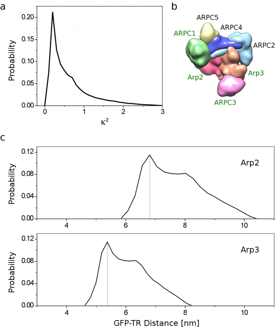
A realistic account of one’s data must include the fact that even if the orientational mobility of the probes is known (from anisotropy data), the relative orientation of the dipoles is not known. That is, if we consider each probe as having a dipole pointed in a specific direction, the mobility of the probe based on the anisotropy measurement tells how much wobble there is in the dipole. This can be approximated as a cone. But one must still consider the many relative directions to which the cones of the donor and acceptor may point. The simplest, but also most complete and fair assessment, is that the relationship of the donor and acceptor orientations may be anything, at random (unless proven otherwise, with a solved structure with the probe in place, for example). Practically speaking, a straightforward way to treat this is to simulate at random all possible relative orientations of donor and acceptor, and for each, to calculate the average κ2 expected based on mobilities from the anisotropy measurements. Grouping the κ2 values from each simulation, a probability distribution of κ2 can be generated (Fig. 4a). This probability distribution can then easily be converted into a probability distribution for the distance for each FRET pair (Fig. 4c, d).
Figure 4. Construction of probability function of FRET distances.
(a) Probability distribution of κ2 calculated from measured anisotropies of donor and acceptor. (b) The seven subunits of the Arp2/3 complex. Arp2/3 constructs with GFP attached to Arp2 (red surface), Arp3 (orange), ARPC1 (green) or ARPC3 (magenta) were used in this study. This view is towards the pointed ends of Arp2 and Arp3. (c) Probability curves for the distances between the Texas red probe (TR) attached to the A site of the CA Scar NPF construct and the center of GFP attached to the C-terminus of Arp2 (top panel) or Arp3 (bottom panel). These curves were derived from FRET under the worst-case scenario assumption that for every donor-acceptor pair in the solution, there was a fixed orientation of donor and acceptor dipoles relative to one another, and the dipoles rotated about this position according to the mobility given by their anisotropies. Note how badly a Gaussian distribution centered at the most probable distance (marked by gray line) would approximate these curves.
Combination of Individual Probability Functions
Once the probability functions for all distances and GFP center locations are derived, they can be combined to form probability functions for each location/distance pair (step 6). The distance probability functions initially form spheres centered at the origin with a profile defined by κ2 (Fig. 4a). To derive the probability function for the probe location for a given the location/distance pair in the common coordinate system, the probability functions need to be convoluted (equation 5). Once convolution was performed, the spheres not only get moved from the origin, they also get distorted from perfect spherical shape because the location probabilities are seldom spherically symmetric (Fig. 5).
Figure 5. Probability function for GFP locations and FRET distance probability functions in common coordinate frame.
(a) Location probability of GFP center when attached to the C-terminus of ARPC1 (green). A low-resolution representation of Arp2/3 complex (gray surface) is shown for reference. There was no electron density attributable to the GFP present in the reconstruction of the corresponding Arp2/3 complex so this distribution is calculated form general constraints (see text). Four orthogonal views are shown, the length of the scale bar is 5 nm. (b) Location probability of GFP center when attached to ARPC3 (magenta). The difference map between the corresponding Arp2/3-GFP construct and the control Arp2/3 complex reconstructions (Fig. 1) was used to calculate this distribution. (c) FRET distance probability distributions for Texas red attached to the A site of the CA Scar NPF construct and GFP attached to ARPC1 (green) or ARPC3 (magenta). These distributions were calculated by mapping the 1D FRET distributions onto a 3D sphere and convoluting it with the GFP location probabilities shown in (a) and (b).
The resulting probability functions for each GFP location/distance pair give information as to where the Texas red label can be, given the experimental constraints for a single GFP. Information from two different GFP labels are independent and defined in the common coordinate system so their probability functions are multiplied voxel-wise in real space (equation 3) to obtain the joint probability function for the combined experimental constraints (step 7).
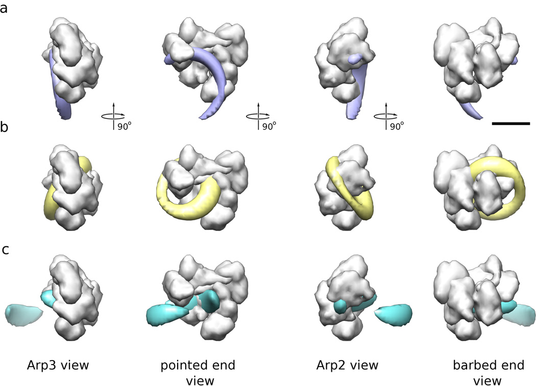
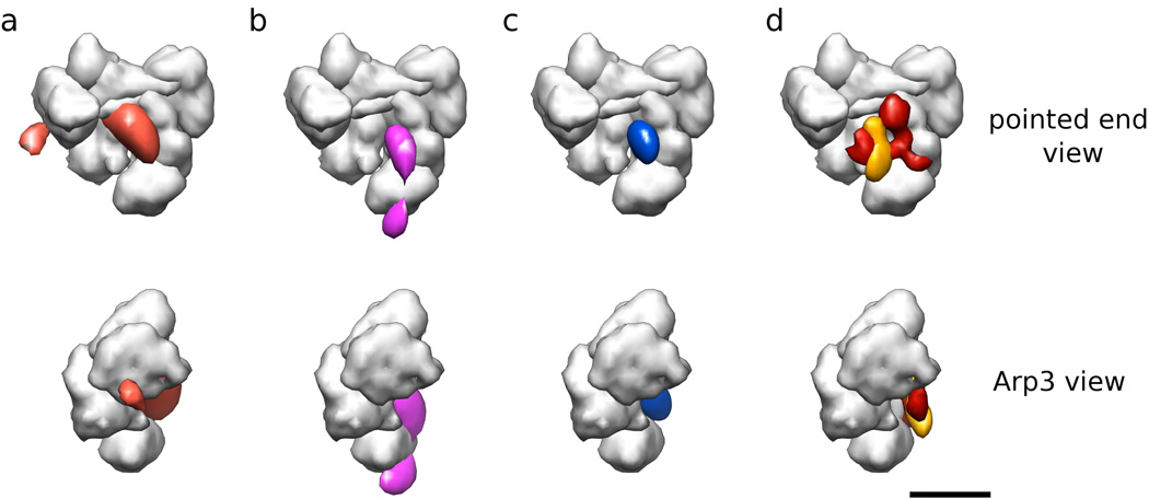
If probability functions of two different GFP labels are combined, the resulting probability function resembles a distorted torus (toroidal from the spherical distance probabilities, distortions from the GFP center location probabilities), that segments into crescent moons at higher contour levels (Fig. 6). If a third GFP label is added, there are already clearly emerging focal points but a secondary peak is also present and/or the peaks are quite elongated (Fig. 7a, b). Addition of the fourth GFP results in a well-defined, single peak, attesting to the high quality of the data and the fact that four FRET pairs are sufficient to uniquely define the a priory unknown position of the Texas red (Fig. 7c).
Figure 6. Joint probability functions for FRET distances in common coordinate frame from two FRET pairs.
(a) Joint probability (blue) of FRET pairs from Texas red attached to the A site of the CA Scar NPF construct and GFP attached to Arp2 and ARPC3. A low-resolution representation of Arp2/3 complex (gray surface) is shown for reference. Four orthogonal views are shown, the length of the scale bar is 5 nm. (b) Joint probability (yellow) of FRET pairs from Texas red attached to the A site of the CA Scar NPF construct and GFP attached to Arp2 and ARPC1. (c) Joint probability (cyan) of FRET pairs from Texas red attached to the A site of the CA Scar NPF construct and GFP attached to ARPC1 and ARPC3.
Figure 7. Joint probability functions for FRET distances in common coordinate frame from multiple FRET pairs.
(a) Joint probability (orange) of FRET pairs from Texas red attached to the A site of the CA Scar NPF construct and GFP attached to Arp2, ARPC1, and ARPC3. A low-resolution representation of Arp2/3 complex (gray surface) is shown for reference. Two orthogonal views are shown. (b) Joint probability (pink) of FRET pairs from Texas red attached to the A site of the CA Scar NPF construct and GFP attached to Arp2, Arp3, and ARPC3. (b) Joint probability (blue) of all four FRET pairs from Texas red attached to the A site of the CA Scar NPF construct and GFP attached to Arp2, Arp3, ARPC1, and ARPC3. The region shown encloses 0.5 of the probability. (d) Difference map calculated from subtraction of the Arp2/3 complex reconstruction from a reconstruction of Arp2/3 complex with bound VCA Scar NPF construct (red) and difference map calculated from subtracting the latter from a reconstruction of the same construct labeled with maltose-binding protein at the V site of VCA (orange). Note the excellent correspondence with the blue probability density in (c). The length of the scale bar is 5 nm.
Interpretation
The interpretation of the probability density functions is relatively straight forward through the use of contour levels. The sum of values inside a certain contour level gives the probability to find the location of the probe within that volume. In the limiting case of a fully determined location without uncertainties, the value of that voxel would be one and that of all others zero. The probability of finding the probe at that location would be one, to find it in any other voxel would be zero. The probability of finding the probe somewhere in the bounding box is always one, which is why it needs to be chosen large enough in the first place. If the sum of probability values within a contour is 0.8, than the probability of the probe being located within that volume is 0.8 and so on.
Validation
The location of the C and A ends of the CA Scar fragment were independently derived by different distance constraints (but the same GFP locations). The locations are both on the same surface of the Arp2/3 complex at a distance of less than 2 nm, fully consistent with the sequence and folding constraints of the CA fragment. In addition, we independently derived the location of the Scar VCA fragment while bound to Arp2/3 complex using EM and difference mapping analysis (Xu et al., 2011) using reconstructions in the absence and in the presence of VCA as well as in the presence of VCA labeled at the V end with maltose-binding protein (Fig. 7d). This allowed us to independently map the location of CA on the surface of the complex at the resolution of the EM study, ~1.9 nm. The centroids of the probability densities are only 0.4 and 1.2 nm away from the surface of the VCA difference density for the A and C labels respectively. This remarkable degree of correspondence between the locations is a strong validation for our probability-based approach.
Conclusions
We presented a method for determining the joint probability function of a priori unknown locations from distance constrains and attachment site information. We applied the method to FRET distances between GFP labels attached to the C-termini of several Arp2/3 complex subunits and a Texas red labels to the C and A ends of a CA nucleation promoting factor fragment to retrieve the location of the bound CA in respect to Arp2/3 complex. Comparison with independent localization of CA by electron microscopy and difference mapping analysis, demonstrates the high fidelity and accuracy of the method. The concept is readily applicable to other types of distance constraints such as cross-linking or NMR dipolar coupling data, allows investigation of the entire probability density landscape, and enables derivation of meaningful confidence intervals.
Acknowledgements
This work was supported by Grant P01 GM066311 from the National Institute of General Medical Sciences to NV.
Footnotes
Publisher's Disclaimer: This is a PDF file of an unedited manuscript that has been accepted for publication. As a service to our customers we are providing this early version of the manuscript. The manuscript will undergo copyediting, typesetting, and review of the resulting proof before it is published in its final citable form. Please note that during the production process errors may be discovered which could affect the content, and all legal disclaimers that apply to the journal pertain.
References
- Brant DA, Flory PJ. The Configuration of Random Polypeptide Chains. I. Experimental Results. J Am Chem Soc. 1965;87:2788–2791. [Google Scholar]
- Brünger AT, Adams PD, Rice LM. Recent developments for the efficient crystallographic refinement of macromolecular structures. Curr Opin Struct Biol. 1998;8:606–611. doi: 10.1016/s0959-440x(98)80152-8. [DOI] [PubMed] [Google Scholar]
- Brünger AT, Strop P, Vrljic M, Chu S, Weninger KR. Three-dimensional molecular modeling with single molecule FRET. J Struc Biol. 2011;173:497–505. doi: 10.1016/j.jsb.2010.09.004. [DOI] [PMC free article] [PubMed] [Google Scholar]
- Chacón P, Morán F, Díaz JF, Pantos E, Andreu JM. Low-resolution structures of proteins in solution retrieved from X-ray scattering with a genetic algorithm. Biophys J. 1998;74:2760–2775. doi: 10.1016/S0006-3495(98)77984-6. [DOI] [PMC free article] [PubMed] [Google Scholar]
- Choi UB, Strop P, Vrljic M, Chu S, Brunger AT, Weninger KR. Single-molecule FRET-derived model of the synaptotagmin 1-SNARE fusion complex. Nat Struct Mol Biol. 2010;17:318–324. doi: 10.1038/nsmb.1763. [DOI] [PMC free article] [PubMed] [Google Scholar]
- Das R, Baker D. Macromolecular modeling with rosetta. Annu Rev Biochem. 2008;77:363–382. doi: 10.1146/annurev.biochem.77.062906.171838. [DOI] [PubMed] [Google Scholar]
- Egile C, Rouiller I, Xu XP, Volkmann N, Li R, Hanein D. Mechanism of filament nucleation and branch stability revealed by the structure of the Arp2/3 complex at actin branch junctions. PLoS Biol. 2005;3:e383. doi: 10.1371/journal.pbio.0030383. [DOI] [PMC free article] [PubMed] [Google Scholar]
- Frauenfelder H, Leeson DT. The energy landscape in non-biological and biological molecules. Nat Struct Biol. 1998;5:757–759. doi: 10.1038/1784. [DOI] [PubMed] [Google Scholar]
- Frauenfelder H, Sligar SG, Wolynes PG. The energy landscapes and motions of proteins. Science. 1991;254:1598–1603. doi: 10.1126/science.1749933. [DOI] [PubMed] [Google Scholar]
- Ha T. Single-molecule fluorescence resonance energy transfer. Methods. 2001;25:78–86. doi: 10.1006/meth.2001.1217. [DOI] [PubMed] [Google Scholar]
- Haas E, Katchalski-Katzir E, Steinberg IZ. Effect of the orientation of donor and acceptor on the probability of energy transfer involving electronic transitions of mixed polarization. Biochemistry. 1978;17:5064–5070. doi: 10.1021/bi00616a032. [DOI] [PubMed] [Google Scholar]
- Habeck M. Statistical mechanics analysis of sparse data. J Struc Biol. 2011;173:541–548. doi: 10.1016/j.jsb.2010.09.016. [DOI] [PubMed] [Google Scholar]
- Holland JH. Adaptation in natural and artificial systems. Ann Harbor, Michigan: University of Michigan Press; 1975. [Google Scholar]
- Kirkpatrick S, Gelatt CD, Vecchi MP. Optimization by simulated annealing. Science. 1983;220:671–680. doi: 10.1126/science.220.4598.671. [DOI] [PubMed] [Google Scholar]
- Pollard TD, Borisy GG. Cellular motility driven by assembly and disassembly of actin filaments. Cell. 2003;112:453–465. doi: 10.1016/s0092-8674(03)00120-x. [DOI] [PubMed] [Google Scholar]
- Rieping W, Habeck M, Nilges M. Inferential structure determination. Science. 2005;309:303–306. doi: 10.1126/science.1110428. [DOI] [PubMed] [Google Scholar]
- Robinson RC, Turbedsky K, Kaiser DA, Marchand JB, Higgs HN, et al. Crystal structure of Arp2/3 complex. Science. 2001;294:1679–1184. doi: 10.1126/science.1066333. [DOI] [PubMed] [Google Scholar]
- Rouiller I, Xu XP, Amann KJ, Egile C, Nickell S, et al. The structural basis of actin filament branching by Arp2/3 complex. J Cell Biol. 2008;180:887–895. doi: 10.1083/jcb.200709092. [DOI] [PMC free article] [PubMed] [Google Scholar]
- Stryer L, Haugland RP. Energy transfer: a spectroscopic ruler. Proc Natl Acad Sci U S A. 1967;58:719–726. doi: 10.1073/pnas.58.2.719. [DOI] [PMC free article] [PubMed] [Google Scholar]
- Timpe L, Peller L. A random flight chain model for the tether of the Shaker K+ channel inactivation domain. Biophys J. 1995;69:2415–2418. doi: 10.1016/S0006-3495(95)80111-6. [DOI] [PMC free article] [PubMed] [Google Scholar]
- van der Meer BW. Kappa-squared: from nuisance to new sense. J Biotechnol. 2002;82:181–196. doi: 10.1016/s1389-0352(01)00037-x. [DOI] [PubMed] [Google Scholar]
- Volkmann N, Hanein D. Quantitative fitting of atomic models into observed densities derived by electron microscopy. J Struc Biol. 1999;125:176–184. doi: 10.1006/jsbi.1998.4074. [DOI] [PubMed] [Google Scholar]
- Volkmann N, Hanein D. Docking of atomic models into reconstructions from electron microscopy. Methods Enzymol. 2003;374:204–225. doi: 10.1016/S0076-6879(03)74010-5. [DOI] [PubMed] [Google Scholar]
- Webb B, Lasker K, Schneidman-Duhovny D, Tjioe E, Phillips J, et al. Modeling of proteins and their assemblies with the integrative modeling platform. Methods Mol Biol. 2011;781:377–397. doi: 10.1007/978-1-61779-276-2_19. [DOI] [PubMed] [Google Scholar]
- Xu XP, Rouiller I, Slaughter BD, Egile C, Kim E, et al. Three-dimensional reconstructions of Arp2/3 complex with bound nucleation promoting factors. EMBO J. 2011;31:236–247. doi: 10.1038/emboj.2011.343. [DOI] [PMC free article] [PubMed] [Google Scholar]


