

Abstract
Problem Addressed
Many pathologies alter the mechanical properties of tissue. Magnetic resonance elastography (MRE) has been developed to noninvasively characterize these quantities in vivo. Typically, small vibrations are induced in the tissue of interest with an external mechanical actuator. The resulting displacements are measured with phase contrast sequences and are then used to estimate the underlying mechanical property distribution. Several MRE studies have quantified brain tissue properties. However, the cranium and meninges, especially the dura, are very effective at damping externally applied vibrations from penetrating deeply into the brain. Here, we report a method, termed ‘intrinsic activation’, that eliminates the requirement for external vibrations by measuring the motion generated by natural blood vessel pulsation.
Methodology
A retrospectively gated phase contrast MR angiography sequence was used to record the tissue velocity at eight phases of the cardiac cycle. The velocities were numerically integrated via the Fourier transform to produce the harmonic displacements at each position within the brain. The displacements were then reconstructed into images of the shear modulus based on both linear elastic and poroelastic models.
Results, Significance and Potential Impact
The mechanical properties produced fall within the range of brain tissue estimates reported in the literature and, equally important, the technique yielded highly reproducible results. The mean shear modulus was 8.1 kPa for linear elastic reconstructions and 2.4 kPa for poroelastic reconstructions where fluid pressure carries a portion of the stress. Gross structures of the brain were visualized, particularly in the poroelastic reconstructions. Intra-subject variability was significantly less than the inter-subject variability in a study of 6 asymptomatic individuals. Further, larger changes in mechanical properties were observed in individuals when examined over time than when the MRE procedures were repeated on the same day.
Cardiac pulsation, termed intrinsic activation, produces sufficient motion to allow mechanical properties to be recovered. The poroelastic model is more consistent with the measured data from brain at low frequencies than the linear elastic model. Intrinsic activation allows MR elastography to be performed without a device shaking the head so the patient notices no differences between it and the other sequences in an MR examination.
Keywords: Magnetic resonance elastography, poroelastic, brain, intrinsic activation
1. INTRODUCTION
Tumors, edema, and other pathologies have different mechanical properties than healthy tissue. Moreover, mechanical property contrast has been found to be significantly higher than other more common contrast mechanisms such as those exploited in magnetic resonance imaging and computed tomography[1–3]. Currently, manual palpation is the most common clinical method of identifying the mechanical differences between pathology and healthy tissue. Quantitative versions of palpation have been realized through ultrasound elastography and magnetic resonance elastography (MRE) which accurately measure the mechanical properties of tissues in vivo[4–7]. In one form of MRE, time-harmonic steady-state mechanical waves are produced within the region of interest and the resulting tissue displacements are measured in 3D at MR resolution[8, 9]. Subsequently, estimates of the tissue’s mechanical properties, most notably the shear modulus, are obtained from these displacements using equations of motion based on an assumed mechanical model (e.g., linear elasticity, viscoelasticity, poroelasticity).
One of the first clinical applications of elastography involved detecting breast lesions[9–11]. More recently, MRE techniques have been applied in the liver[12], muscle, footpads, prostate, heart, and brain[13–18]. While MRE of the liver has proven most successful to date, significant effort has been devoted to understanding the mechanical properties of brain tissue because of the number of important neuropathologies that alter its characteristics. For example, Alzheimer’s disease results when the healthy fatty myelin sheath is replaced with a stiffer amyloid plaque. Hydrocephalus is characterized by an increase in intracranial pressure (ICP), often caused by a blockage in the lateral ventricles. Cerebrospinal fluid (CSF) accumulates in the ventricles causing ventricular expansion and heightened ICP. A compilation of healthy brain tissue stiffness estimates appears in Kruse et al.[19] and indicates a range from 1–35 kPa, with MRE reporting values from 1–14 kPa. One contributor to the variability could be the difficulty in mechanically actuating tissue deep in the brain. Brain tissue is enveloped in three layers of cerebral meninges, CSF, and the skull, all of which help to isolate the parenchyma from external vibrations. Some studies such as Kruse et al.[19] designate areas of low motion as unreliable data and remove these regions from analyses. Low motion results in poor signal-to-noise ratio that typically degrades the estimates of mechanical properties from displacement measurements.
To overcome the challenge of brain tissue actuation, we have developed an MRE technique based on intrinsic motion caused by blood pressure pulses during the cardiac cycle. A similar method has been reported by Zhao et al.[20], where brain tissue velocity is fit to a damped oscillation model to estimate the mechanical wave speed and associated shear modulus. Our approach measures tissue displacements at multiple cardiac phases through a standard, retrospectively gated, multiphase MR angiography phase-contrast acquisition that is able to capture tissue velocities at MR resolution. The velocities are integrated over time to retrieve the corresponding displacements, which are processed through the identical procedures used in conventional externally actuated MRE. Here, we describe the technique and report our initial shear modulus estimates from human studies of healthy brain.
The results are promising on several fronts. First, we show that motion can be observed throughout the brain using standard MR pulse sequences without the aid of an external actuator. Second, the temporal dynamics of the blood pulsation waveform produced a sufficiently robust time-harmonic motion signal that allowed for repeatable estimates of the 3D spatial distribution of the shear modulus throughout the acquisition volume using algorithms developed for time-harmonic MRE at much higher externally actuated frequencies (~100 Hz). Third, the generation of reproducible spatially-resolved shear modulus distributions from motion caused by intrinsic activation allows MRE to pursue a myriad of neuropathologies and to begin to classify different disease characteristics. Fourth, intrinsic activation makes the examination just as comfortable as a normal MRI procedure so a much wider cross-section of patients can be studied.
2. MATERIAL AND METHODS
MR elastography involves three processes: 1) mechanical actuation (vibration) of the tissue of interest, 2) measurement of the resulting tissue displacements, and 3) estimation of the tissue mechanical properties from the displacement data. Here, we summarize the methods used to record motion in brain tissue from vibrations induced by intrinsic cardiac pulsation and convert the displacement information into maps of brain mechanical properties.
2.1 Motion Encoding
The cardiac cycle has periods of approximately one-second. As a result, the common method of motion encoding with sinusoidal gradients applied during the motion[6] is no longer possible because echo times approaching one-second leave no signal. However, fractional encoding techniques[21, 22] can be applied to allow the sinusoidal motion to be found by encoding part of the motion cycle. While the phase difference signal is significantly smaller, it is compensated by a much higher signal due to the shorter echo times. The displacements at each position were then calculated from the measured velocities.
To encode motion from intrinsic activation, subjects were placed supine in an eight-channel phased array head coil on a Philips Achieva 3.0 T scanner. A multiphase, phase-contrast, gradient echo, angiographic sequence was set for maximum sensitivity to motion allowing a maximum velocity of 2.5 cm/sec to be recorded without aliasing. Eight cardiac phases were measured using retrospective gating synchronized to a pulse oximeter placed on the subject’s finger. The heart rate was stable for the healthy volunteers participating in these exams and provided a consistent trigger signal when sensed through the pulse oximeter, which was simple to apply. No adjustments for heart rate variations were considered, although acquisitions from patients with very irregular rates might require some compensation and be better gated through an ECG. The voxel size was 1 mm × 1 mm × 3 mm and 16 slices were acquired during each examination. The repetition time was 14.5 msec and the echo time was 12.4 msec. The acquisition time for each motion direction depended on heart rate but required approximately 8 minutes yielding a total exam time of less than 30 minutes.
The harmonic displacements at each position, u, were recovered from the measured velocities, u̇, by integration. Integration is relatively simple to perform in the Fourier domain by dividing by the frequency:
| (1) |
where ω is the frequency of mechanical actuation and is the Fourier transform. In this work we only used the Fourier coefficient for the fundamental frequency, which provided a least squares estimate of the sinusoidal portion of the motion at this frequency. Thus, the harmonic displacements were obtained from a conventional phase contrast angiography sequence that produces velocity estimates at multiple phases of the cardiac cycle.
2.2 Mechanical Parameter Estimation
The displacements were then used to estimate the shear modulus with both linearly elastic [23, 24] and poroelastic [25, 26] models. The linear elastic equations of motion characterize tissue through the shear modulus, μ, and the other Lamé constant λ:
| (1) |
where is the vector of displacements and ρ is the density. In equation (1), the double-dot superscript denotes a second derivative in time and the T superscript indicates matrix transposition. The poroelastic model includes the effects of fluid moving through pores in an elastic solid matrix. It characterizes the tissue with μ and λ for the solid matrix and the ease with which the fluid is able to move through the matrix. The time-harmonic form of the governing equations are given by:
| (2) |
| (3) |
and
| (4) |
where and p are the complex-valued amplitudes of the displacement and pressure on the fluid, respectively, ω is the actuation frequency, ρf is the fluid density, ρa is the apparent mass density and β is a compilation of poroelastic parameters: κ is the hydraulic conductivity (the ease at which fluid moves through the pores) and ϕ is the porosity (the volume fraction of pore space to total volume).
These methods use the measured displacement field interpolated onto a finite element mesh with 2–3 mm nodal spacing. The shear modulus distribution is determined by a nonlinear, least squares fit between the measured displacements and those calculated by the governing equations of motion using an iterative subzone-based optimization[23, 24]. Each subzone is computed in parallel allowing inversion of the full 3D brain in approximately two hours. The poroelastic model has been argued to represent the brain more accurately than other governing equations[27] because the tissue is described as a biphasic material consisting of an elastic solid matrix saturated with an infiltrating incompressible pore fluid. The biphasic equations allow an estimate of both the elastic properties of the solid tissue matrix and the amplitude of the time-harmonic pore fluid pressure. No extra filtering of the velocity or displacement data was employed.
2.3 Technique Evaluation
To evaluate this method, we imaged healthy subjects multiple times (3–5) over a period of time ranging from 9 to 45 weeks. The study involved six subjects (four male, two female) ranging from 25 to 55 years of age. To investigate the reproducibility and accuracy of the technique, we also imaged three of the subjects three times in succession without movement between scans. Reproducibility was measured via the coefficient of variation (CoV), which is the ratio of the standard deviation of the sample set over the mean of the same set.
To remove partial volume effects, the acquired images from scans acquired from one subject over multiple days were aligned using an unsupervised rigid rotation and translation that optimized the alignment of the skull in the image sets. Only the common volume among the scans for each subject was used to estimate the mean shear moduli. In addition, the average mechanical properties between grey and white matter were compared. These areas were segmented from the intensity values of a corresponding T2-weighted MR image with the same field-of-view as the acquired displacement data.
3. RESULTS
The reconstructed images had little motion artifact indicating that the gating was adequate. The pattern of periodic motion induced in the brain by cardiac pressure pulsations, an example of which is shown in Figure 1, was characterized to establish the potential of intrinsic activation to sample the full cranial volume. The reproducibility of the reconstructed mechanical properties was evaluated and values of shear modulus were compared with the literature. In addition, the linear elastic and poroelastic reconstructions were briefly compared.
Figure 1.
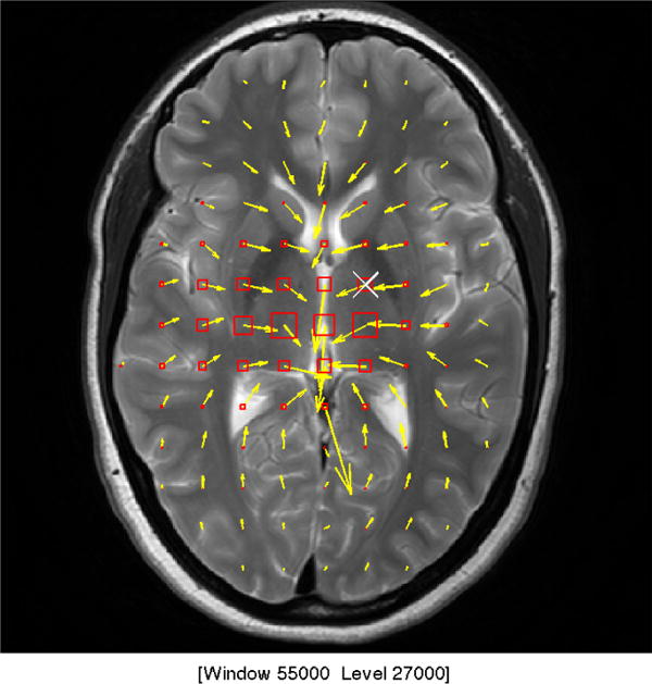
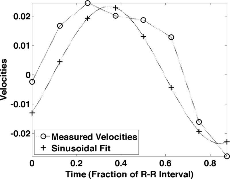
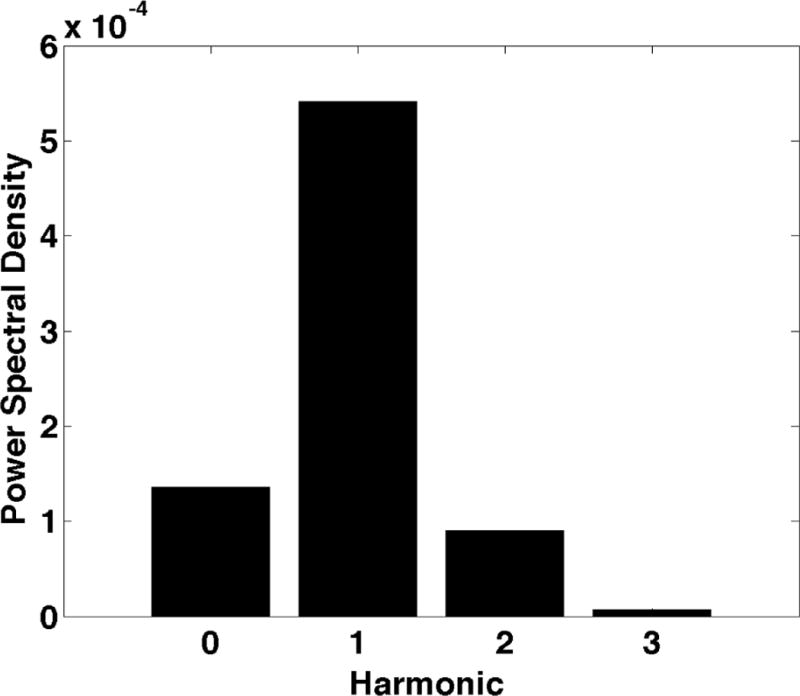
a) shows the sinusoidal components of the motion induced by cardiac pulsation, termed intrinsic activation. The motion for the first examination of Subject F is shown during systole. The in plane motion is represented by the yellow arrows where longer arrows represent larger motion. The through plane motion is represented by the boxes where the larger motion is represented by a larger box and red represents inferior motion and yellow represents superior motion. b) shows the measured velocities in the superior-inferior direction with the least squares sinusoid. c) shows the power spectral density of the measured motion at the point marked with the white “X” in Fig. 1a and plotted in Fig. 1b.
Figure 2 shows average motion magnitude (in microns) across all exams for each subject in four regions of the brain with varying proximity to the Circle of Willis, where interventional radiologists observe the largest pulsatility. Regions 1 and 2 were encompassed in the five most inferior slices, which were closest to the Circle of Willis whereas Regions 3 and 4 were isolated to the five most superior slices, which were farthest from the Circle of Willis. Regions 1 and 3 included the central portion of the brain (and were within a 22 mm radius from the center) while Regions 2 and 4 were more than 22 mm from the center of the brain. Region 1 included the Circle of Willis. Regions 2, 3 and 4 were in the peripheral parenchyma. Voxels with CSF were eliminated from the analysis of all regions. For all subjects, the largest motion was generated in the region surrounding the Circle of Willis (Region 1) rather than in the peripheral parenchyma where the largest blood pressure drop occurs[28]. A two-sided, paired t-test was used to compare the magnitude of the average motion in the four regions across all acquisitions in all subjects. The p-value for the null hypothesis that the motion magnitude in Region 1 was the same as in the other regions was less than 10−13. Average motion magnitudes in Regions 2 and 3 were very similar: the p-value from the paired t-test was 0.27 and, conversely, the correlation coefficient measuring the similarity in motion magnitude was 0.76 with a p-value of 0.0003. The average motion magnitude in Region 4 was significantly different from Regions 2 and 3 with paired t-test p-values of 4 × 10⁻⁹ and 3 × 10⁻⁶, respectively.
Figure 2.
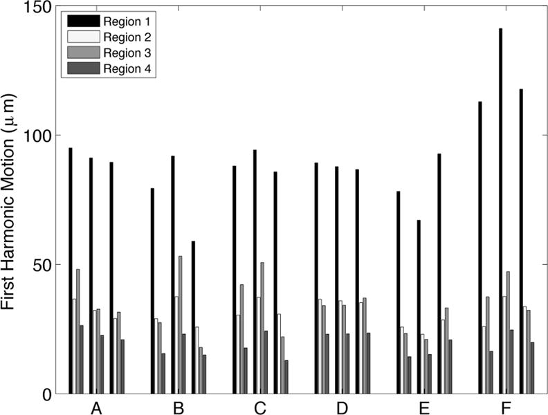
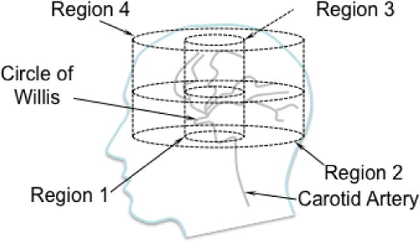
a) shows the average motion in four regions of the brain for the three repeated MRE exams for Subjects A through F. Region 1 was within a 22 mm radius of the center of the brain in the most inferior five slices, which is closest to the Circle of Willis; Region 2 was beyond the 22 mm radius in the most inferior five slices; Region 3 was inside the 22 mm radius on the most superior five slices; Region 4 was outside the 22 mm in plane radius in the most superior five slices. The motion is highest in region 1, nearest to the Circle of Willis. The four cylindrical regions of interest are depicted in relation to the Circle of Willis in the line drawing shown in b).
Table 1 summarizes the mean and standard deviation of the shear modulus estimates for linear elastic inversion (LEI) and poroelastic inversion (PEI) for the subject data taken over several days. The mean shear modulus for LEI was 8.14 kPa whereas it was significantly smaller (p<0.01) for PEI at 2.34 kPa. LEI estimates fall on the higher end of literature values for brain tissue at frequencies ranging from 25–100Hz, while the PEI estimates occur within a much more populated span of the stiffnesses reported. While this comparison ignores any viscoelastic effects that may be present, it shows that the results are within an expected range of stiffness values. Further, averages were taken of the individual standard deviations of the shear moduli estimates to characterize the overall variability of a specific mechanical model. The LEI reconstructions had a coefficient of variation (CoV) of 27.4% whereas the CoV of PEI reconstructions was much less at 8.25%. Figure 3 shows two examples of the different model estimates for the same series of 2D slices. In both cases, the linear elastic algorithm has very little spatial information, much higher variability within a single slice, and also lacks hemispherical symmetry. The bottom row of Figure 3 presents the corresponding PEI estimates where more spatial information is evident, as well as much lower variation and much better symmetry. Specifically, the ventricles (which should have very low shear modulus because fluid cannot withstand a shear stress) are not apparent in the LEI estimate for Subject C and vaguely appear in Subject D in column 1 and only slightly in column 2, whereas the ventricles are easily found in the PEI estimates of both subjects.
Table 1.
Linear elastic (μLE) and poroelastic (μPE) estimates of shear modulus for human brain tissue. The standard deviations (SD) reflect the average standard deviation for aligned images. The mean values are averaged over the entire reconstructed volume of the brain. All datasets were acquired on different days.
| Subject | μLE (Pa) | μPE (Pa) | ||
|---|---|---|---|---|
| Mean | SD | Mean | SD | |
| A | 7192 | 1603 | 2381 | 214 |
| B | 8546 | 2375 | 3018 | 385 |
| C | 6755 | 735 | 2229 | 111 |
| D | 8032 | 4339 | 1925 | 235 |
| E | 9301 | 2508 | 2110 | 131 |
| F | 8984 | 1817 | 2364 | 82 |
| Total | 8135.1 +/− 1005.2 | 2229.6 +/− 1212.0 | 2337.5 +/− 373.88 | 193.05 +/− 111.31 |
Figure 3.
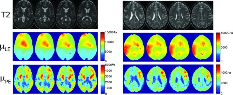
Four transverse brain slices of two subjects (C and D, respectively) illustrated with T2-weighted MRI (top row) and corresponding shear modulus images with linear elastic (μLE, second row) and poroelastic (μPE, third row) inversions (colorbar in Pascals). T2-weighted images have TR=3700ms, TE=100ms.
The reproducibility of the PEI shear modulus estimates was examined as a function of inter-subject (between subjects) and intra-subject (within a single subject) variability. The inter-subject variability was calculated by taking the CoV of the individual subject mean shear moduli. Intra-subject variability involved averaging the CoV of each subject. Inter-subject CoV was 16.0% and intra-subject CoV was 8.1%. An example of the same slices acquired on separate days is shown in Figure 4, with each row corresponding to a new MRE session with the same coregistered volume. Another reproducibility test was examined by comparing the studies performed on a single day with those occurring over longer periods of time. Table 2 shows that CoV decreased for repeat studies conducted on the same day when compared to CoVs for scans repeated over several weeks, decreasing from an average CoV of 8.1% over weeks to 4.8% on a single day.
Figure 4.
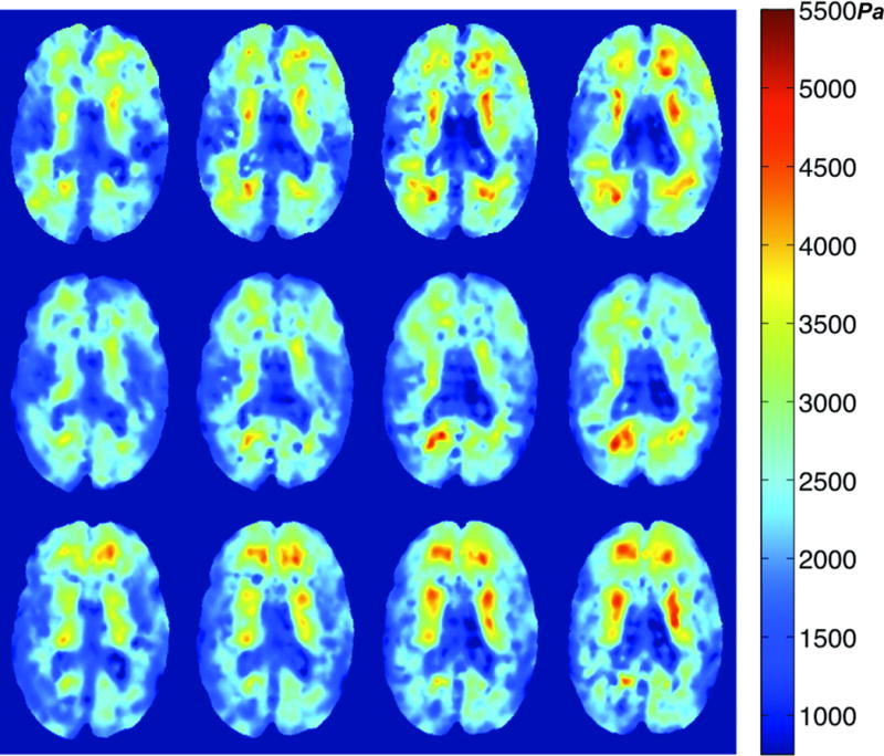
PEI Shear modulus images from three different sessions of Subject F. Each row corresponds to a different MRE exam. The four transverse slices in a given row represent the same locations within the coregistered image volumes. All three sessions provide similar property values and distributions, as well as delineation of the ventricles. Scale is in Pascals.
Table 2.
Poroelastic (μPE) estimates of shear modulus (in Pa) for MRE exams conducted on separate days versus values from sessions performed consecutively on the same day (denoted RS for repeat study). Values reflect the mean and standard deviation for aligned images. Repeatability is categorized by the coefficient of variation (CoV), which is the ratio of the standard deviation and the mean.
| Subject | Mean (Pa) | SD (Pa) | CoV (SD/Mean) |
|---|---|---|---|
|
A RSA |
2381 2447 |
214.3 156.6 |
9.00% 6.39% |
|
C RSC |
2228 2117 |
111.2 55.96 |
4.99% 2.64% |
|
D RSD |
1925 2105 |
235.2 99.67 |
12.2% 4.73% |
|
E RSE |
2109 2146 |
131.2 114.2 |
6.22% 5.32% |
The average shear moduli within grey matter and white matter was compared across the six subjects as shown in Figures 5 and 6. Figure 5 indicates the intensity-based MR segmentation used to gather shear modulus data for the two parenchymal tissue types. Figure 6 summarizes the means and standard deviations of the grey and white matter estimates in each subject. A paired t-test for the hypothesis that the mean shear modulus within the two ROIs for each subject is the same was performed. The average shear modulus within the two ROIs was significantly different for each subject with p-values ranging from 10−2–10−7. The average difference between the two regions was 268.8 Pa, or 11.5% of the total mean shear modulus of tissue.
Figure 5.
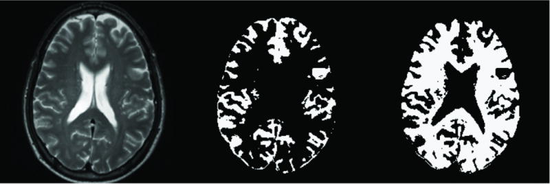
Representative transverse T2-weighted MR image (left) with the corresponding MR-intensity based binary segmentation of grey (middle) and white (right) matter.
Figure 6.
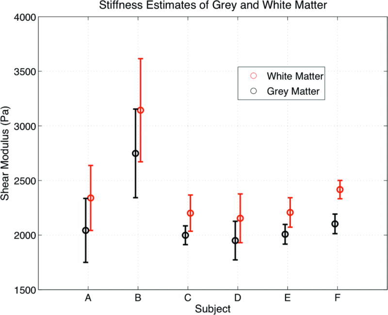
Average shear modulus within the segmented grey and white matter areas (shown in Fig. 5) averaged over the studies for each subject plotted using the standard deviation of the shear modulus within the ROIs. The scale is in Pascals.
4. DISCUSSION
Intrinsic activation is potentially a very important advance in brain MRE because it minimizes the impact of two of the biggest disadvantages of current techniques – 1) cumbersome external actuators and 2) poor shear wave penetration. Measuring tissue motion based on intrinsic pulsations puts MRE on equal footing with other MR sequences from the patient, technologist and clinical procedure perspectives; thus, allowing quantitative estimates of brain tissue properties to be obtained as part of other studies through an additional acquisition which involves largely standard practices. Further, the technique spatially distributes the generation of motion through the central core of the brain rather than relying on the propagation of wavefronts throughout the cranial volume, which originate from the peripheral surfaces of the parenchyma when the head is vibrated externally.
The cardiac pulsation motion in healthy brain begins around the Circle of Willis and propagates out from that region. We found that the motion in the region around the Circle of Willis was significantly larger than in other parts of the brain. The motion in the peripheral region of the most inferior slices was also similar to that in the central region of the most superior slices. Importantly, the motion amplitude did not decrease by more than a factor of five from the central region to the most superior peripheral tissues and generated sufficient displacements to reconstruct mechanical property estimates reproducibly throughout the brain. The central distribution of the motion indicates that most of the tissue displacement is induced by pulsation around the Circle of Willis. Externally induced motion reported in other MRE applications, where the displacements were generated by external vibrations, ranges from 10 μm to 1 mm[18, 19]. The harmonic motion component we measured through the intrinsic actuation method described here ranged from 10 μm to 100 μm but is only a portion of the total pulsatile motion, which has been reported to be in the range 50 μm to 150 μm[29].
The gross features of the brain in the shear modulus maps correlate well with the underlying anatomy and possess good symmetry in PEIs more so than their LEI counterparts. For example, in Figure 3 the ventricles in the linear elastic estimates are less uniformly low in shear modulus, but have the expected low shear modulus in the PEI. Several regions of high shear also occur in the LEI that were not expected, specifically the high shear values appearing anterior to the ventricles, likely caused by model-data mismatch. Their absence in the PEI suggests that poroelasticity is likely a more appropriate representation of brain tissue than linear elasticity. Also, LEI lacks symmetry in the hemispheres, whereas the PEI images present much more noticeable symmetry. For instance, in the first column of Figure 3, the PEI image has a higher stiffness area in the periventricular parenchyma in both hemispheres. The variability study on the series of subjects also supports this view. The CoV of the LEI estimates was significantly higher than the corresponding PEI estimates (27.4% and 8.25%, respectively), demonstrating that the PEI algorithm handles this type of motion data better than its LEI counterpart. Both models assume the measured displacement field is induced by an externally-driven source of motion. The absence of artifact adjacent to the ventricles indicates that the assumption is adequate for representing the tissue motion in the model.
The linear elastic results (averaging 8.14 kPa) fall within the 5 kPa to 15 kPa range at 100 Hz reported for human brain in Kruse et al.[19] and for feline brain in Pattison et al.[30] but are stiffer than shear moduli measured by other groups which are lower (1–3 kPa)[31, 32]. A quantitative comparison at different frequencies is not possible without assuming a dispersion relationship, but lower shear modulus values are generally expected for lower frequencies. The PEI results (averaging 2.34 kPa) appear to be more consistent in this regard because LEIs tend to overestimate the shear modulus of a biphasic material[26].
The CoVs found for inter-subject and intra-subject variation illustrate that our intrinsically actuated MRE technique can detect more differences in brain parenchyma throughout a population than in a single subject, which supports the expected outcome that a healthy brain does not change its mechanical property signature as widely as the mechanical properties of an array of brains from individuals of different age and sex. Furthermore, the shear modulus in the grey and white matter was significantly different (p<10−2–10−7) in the six subjects. This finding supports the contention that the high contrast within the brain correlates well with its structural architecture. It also agrees with the results presented previously using the subzone-based optimization algorithm for feline brains[30]. Interestingly, although a detectable, statistically-significant difference exists, our results indicate that the bulk mechanical properties of gray and white matter are not dramatically different (<20%).
While the results reported in this paper are promising, intrinsic activation needs to be investigated and optimized further on several fronts. In conventional MRE, the externally-created motion driving waveform is a simple sinusoid, whereas motion produced by cardiac pulsation is not purely sinusoidal. The latter follows the arterial pressure cycle, which is smoother and more uniform than electroencephalography signals, but is still not a sine wave.
In addition, the presence of large vessels within the motion measurement volume was not debilitating. The measured motion in voxels containing a significant proportion of fast moving blood can easily produce aliased motion estimates because of the high sensitivity to motion required to measure the small tissue velocities. The extent of the aliasing depends on the proportion of the voxel occupied by moving blood and how fast the blood is moving, which may become a more significant challenge when higher spatial resolution is employed. The current 1 mm × 1 mm × 3 mm voxels did not present significant problems with aliasing. If aliasing does become an issue, another phase contrast data set acquired to measure large velocities would allow the smaller velocities to be measured without aliasing.
Another aspect of intrinsic activation for further study is whether the presence of small arteries distributed throughout the parenchyma should be represented as a forcing term during image reconstruction. The models used here were developed for externally vibrated tissue that is deformed from its surface not tissue with forced internal expansion. The arterial system is branched from the Circle of Willis to arteries in the parenchyma, most of which travel on the surface of the brain. However, a few, such as the middle cerebral artery, are deeper and may prove to be the source of enough motion to necessitate the addition of a distributed forcing term in the equations of motion. The results presented in this study appear to be of sufficient quality to suggest that the arteries are small enough to allow the current models to be used.
The elimination of specialized mechanical actuation equipment and the use of generally available pulse sequences places brain MRE based on intrinsic activation in the hands of the vast majority of clinical installations. The only remaining impediment is the reconstruction software, which can typically be disseminated or obtained through collaborations much more readily than specialized hardware and pulse sequences because of its scanner platform independence. Intrinsic activation of the brain also makes the MRE study no more onerous than most any other MR examination, expanding significantly the patient population able to undergo the procedure which should allow brain MRE to be investigated more rapidly in a much wider venue of neuroimaging applications.
4. CONCLUSIONS
Mechanical properties of the brain can be estimated from intrinsic activation caused by blood pressure pulsation during the cardiac cycle, eliminating the need for externally induced vibrations. The motion is primarily generated in the region around the Circle of Willis but it is transmitted throughout the parenchyma with sufficient amplitude to allow repeatable and stable estimates of mechanical properties throughout the image acquisition volume. Importantly, the mechanical properties obtained are reproducible and consistent with values presented in the literature, especially when poroelastic inversion methods were used. The temporal reproducibility of repeated studies was smaller than the spatial variation in shear modulus observed in the individual. The reproducibility was also significantly smaller than the mechanical property changes caused by abnormalities, which suggests that variations arising from the outcome of therapies and/or the progression of disease can be monitored longitudinally.
Acknowledgments
This work was supported by NIH Grant 5 R01 EB004632-04.
References
- 1.Duck F. Physical properties of tissue: a comprehensive reference book. San Diego, CA: Academic Press; 1990. [Google Scholar]
- 2.Doyley MM, et al. Thresholds for detecting and characterizing focal lesions using steady-state MR elastography. Medical Physics. 2003;30(4):495. doi: 10.1118/1.1556607. [DOI] [PubMed] [Google Scholar]
- 3.Venkatesh SK, et al. MR Elastography of Liver Tumors: Preliminary Results. American Journal of Roentgenology. 2008;190:1534–1540. doi: 10.2214/AJR.07.3123. [DOI] [PMC free article] [PubMed] [Google Scholar]
- 4.Parker K, et al. Tissue response to mechanical vibrations for “sonoelasticity imaging”. Ultrasound in Medicine and Biology. 1990;16(3):241–246. doi: 10.1016/0301-5629(90)90003-u. [DOI] [PubMed] [Google Scholar]
- 5.Ophir J, et al. Elastography: A Quantitative Method for Imaging the Elasticity of Biological Tissues. Ultrasonic Imaging. 1991;13:111–134. doi: 10.1177/016173469101300201. [DOI] [PubMed] [Google Scholar]
- 6.Muthupillai R, et al. Magnetic resonance elastography by direct visualization of propagatin acoustic strain waves. Science. 1995;269(5232):1854–1857. doi: 10.1126/science.7569924. [DOI] [PubMed] [Google Scholar]
- 7.Muthupillai R, Ehman RL. Magnetic resonance elastography. Nature Medicine. 1996;2(5):601–603. doi: 10.1038/nm0596-601. [DOI] [PubMed] [Google Scholar]
- 8.Weaver JB, et al. Magnetic resonance elastography using 3D gradient echo measurements of steady-state motion. Medical Physics. 2001;28(8):1620–1628. doi: 10.1118/1.1386776. [DOI] [PubMed] [Google Scholar]
- 9.Sinkus R, et al. High-resolution tensor MR elastography for breast tumour detection. Physics in Medicine and Biology. 2000;45:1649–1664. doi: 10.1088/0031-9155/45/6/317. [DOI] [PubMed] [Google Scholar]
- 10.Garra BS, et al. Elastography of breast lesions: initial clinical results. Radiology. 1997;202:79–86. doi: 10.1148/radiology.202.1.8988195. [DOI] [PubMed] [Google Scholar]
- 11.McKnight AL, et al. MR Elastography of Breast Cancer: Preliminary Results. AJR. 2002;178:1411–1417. doi: 10.2214/ajr.178.6.1781411. [DOI] [PubMed] [Google Scholar]
- 12.Dresner MA, et al. MR Elastography of the Liver: Preliminary Results. Radiology. 2006;240(2):440–448. doi: 10.1148/radiol.2402050606. [DOI] [PubMed] [Google Scholar]
- 13.Dresner MA, et al. Magnetic Resonance Elastography of Skeletal Muscle. Journal of Magnetic Resonance Imaging. 2001;13:269–276. doi: 10.1002/1522-2586(200102)13:2<269::aid-jmri1039>3.0.co;2-1. [DOI] [PubMed] [Google Scholar]
- 14.Kemper J, et al. MR elastography of the prostate: initial in-vivo application. RoFo : Fortschritte auf dem Gebieteder R□ontgenstrahlen und der Nuklearmedizin. 2004;176(8):1094–1099. doi: 10.1055/s-2004-813279. [DOI] [PubMed] [Google Scholar]
- 15.Weaver JB, et al. Imaging the Shear Modulus of the Heel Fat Pads. Clinical Biomechanics. 2005;20:312–319. doi: 10.1016/j.clinbiomech.2004.11.010. [DOI] [PubMed] [Google Scholar]
- 16.Rouvière O, et al. MR Elastography of the Liver: Preliminary Results. Radiology. 2006;240:440–448. doi: 10.1148/radiol.2402050606. [DOI] [PubMed] [Google Scholar]
- 17.Green MA, Bilston LE, Sinkus R. In vivo brain viscoelastic properties measured by magnetic resonance elastography. NMR in Biomedicine. 2008;21:755–764. doi: 10.1002/nbm.1254. [DOI] [PubMed] [Google Scholar]
- 18.Sack I, et al. The impact of aging and gender on brain viscoelasticity. NeuroImage. 2009;46:652–657. doi: 10.1016/j.neuroimage.2009.02.040. [DOI] [PubMed] [Google Scholar]
- 19.Kruse SA, et al. Magnetic resonance elastography of the brain. NeuroImage. 2008;39:231–237. doi: 10.1016/j.neuroimage.2007.08.030. [DOI] [PMC free article] [PubMed] [Google Scholar]
- 20.Zhao S, Jackson A, Parker GJ. Auto-elastography of the brain. Proceedings of the ISMRM. 2009;39 [Google Scholar]
- 21.Rump J, et al. Fractional encoding of harmonic motions in MR-elastography. Magn Reson Med. 2007;57:388–395. doi: 10.1002/mrm.21152. [DOI] [PubMed] [Google Scholar]
- 22.Rump J, et al. Phase preparation in steady-state free precession MR elastography. Magn Reson Imaging. 2008;26:228–235. doi: 10.1016/j.mri.2007.07.009. [DOI] [PubMed] [Google Scholar]
- 23.Van Houten EEW, et al. Three-Dimensional Subzone-Based Reconstruction Algorithm for MR Elastography. Magnetic Resonance in Medicine. 2001;45:827–837. doi: 10.1002/mrm.1111. [DOI] [PubMed] [Google Scholar]
- 24.Van Houten EE, et al. An Overlapping Subzone Technique for MR-Based Elastic Property Reconstruction. Magnetic Resonance in Medicine. 1999;42:779–786. doi: 10.1002/(sici)1522-2594(199910)42:4<779::aid-mrm21>3.0.co;2-z. [DOI] [PubMed] [Google Scholar]
- 25.Perrinez PR, et al. Modeling of Soft Poroelastic Tissue in Time-Harmonic MR Elastography. IEEE Transactions on Biomedical Engineering. 2009;56(3):598–608. doi: 10.1109/TBME.2008.2009928. [DOI] [PMC free article] [PubMed] [Google Scholar]
- 26.Perrinez PR, et al. Magnetic resonance poroelastography: an algorithm for estimating the mechanical properties of fluid-saturated soft tissues. IEEE transactions on medical imaging. 2010;29(3):746–755. doi: 10.1109/TMI.2009.2035309. [DOI] [PMC free article] [PubMed] [Google Scholar]
- 27.Franceschini G, et al. Brain tissue deforms similarly to filled elastomers and follows consolidation theory. Journal of the Mechanics and Physics of Solids. 2006;54:2592–2620. [Google Scholar]
- 28.Guyton . Textbook of Medical Physiology. Philadelphia PA: W. B. Saunders Company; 1986. [Google Scholar]
- 29.Soellinger M, et al. 3D Cine Displacement-Encoded MRI of Pulsatile Brain Motion. Magnetic Resonance in Medicine. 2009;61:153–162. doi: 10.1002/mrm.21802. [DOI] [PubMed] [Google Scholar]
- 30.Pattison AJ, et al. 3D-time harmonic magnetic resonance elastography of the healthy feline brain. Journal of Biomechanics. 2010;43:2747–2752. doi: 10.1016/j.jbiomech.2010.06.008. [DOI] [PMC free article] [PubMed] [Google Scholar]
- 31.Murphy M, et al. Decreased brain stiffness in alzheimer’s disease determined by magnetic resonance elastography. Journal of magnetic resonance imaging. 2011;34:494–498. doi: 10.1002/jmri.22707. [DOI] [PMC free article] [PubMed] [Google Scholar]
- 32.Streitberger KJ, et al. In vivo viscoelastic properties of the brain in normal pressure hydrocephalus. NMR in Biomedicine. 2010;24(4):385–392. doi: 10.1002/nbm.1602. [DOI] [PubMed] [Google Scholar]