

Abstract
Microscopic sessile suspension feeders are a critical component in aquatic ecosystems, acting as an intermediate trophic stage between bacteria and higher eukaryotic taxa. Because they live attached to boundaries, it has long been thought that recirculation of the feeding currents produced by sessile suspension feeders inhibits their ability to access fresh fluid. However, previous models for the feeding flows of these organisms assume that they feed by pushing fluid perpendicular to surfaces they live upon, whereas we observe that sessile suspension feeders often feed at an angle to these boundaries. Using experiments and calculations, we show that living suspension feeders (Vorticella) likely actively regulate the angle that they feed relative to a substratum. We then use theory and simulations to show that angled feeding increases nutrient and particle uptake by reducing the reprocessing of depleted water. This work resolves an open question of how a key class of suspension-feeding organisms escapes physical limitations associated with their sessile lifestyle.
Introduction
Any pebble, leaf, or even animal taken from a pond or ocean will host a myriad community of microscopic sessile suspension feeders (1,2). These microscopic organisms live attached to underwater surfaces and form an essential link in the aquatic carbon chain by consuming bacteria and small detritus and then, in turn, being eaten themselves by larger organisms (3–6). As consumers of bacteria, they also play a key role in processing waste-water in treatment plants (7,8), and may also improve degradation of contaminants from human-caused environmental disasters, such as oil spills and sewage leaks (9–12). Choanoflagellates, one type of suspension feeder that is primarily sessile (13), have been estimated to filter between 1 and 25% of the sea water in coastal areas each day (6,14). Some estimates suggest that every fluid particle in such coastal areas may pass through the filtering apparatus of a suspension feeder at least once per day (14–17), and approximately half of the suspension feeders considered in those estimates live permanently or temporarily attached to substrates (17). Such estimates of sea water filtration enhance our understanding of the contributions of sessile filter feeders to the ecology of these systems and possibly to the effective cleanup of human-introduced contaminants. However, some of these estimates rely on measurements of fluid flow near organisms that may not mimic fluid flow in natural environments (16).
Microscopic suspension feeders, such as Stentor (18), Opercularia (19), and choanoflagellates (6) are ∼1 μm to a few hundred μm in size and are composed of one to a few cells. They use the motion of cilia or flagella to draw fluid toward themselves and feed from the passing fluid (20–22). These organisms live in the regime of low Reynolds number flow, which means that viscous forces dominate and inertia is negligible (23). The Reynolds number represents the ratio of inertial to viscous forces and is defined as Re = ρUL/μ, where ρ is the density of the fluid, U and L are typical velocity and length scales, respectively, and μ is the viscosity of the fluid. For a typical suspension feeder, Vorticella, Re ≈ 5 × 10⁻³. In this article, we focus on Vorticella as a model for many similar surface-attached organisms.
Feeding at a small distance above a boundary in low Reynolds number flow creates two challenges:
-
1.
Viscous drag from the surface slows down the feeding currents generated compared to those in free space, leading to less efficient feeding (13,24); and
-
2.
Viscous eddies (i.e., regions of closed streamlines) created by the interaction of filter feeding currents with the boundary recirculate fluid past the feeding apparatus even after nutrients have been removed (19,25–28).
For most sessile filter feeders, the effect of the first challenge (viscous drag from the surface) is reduced greatly by moving the cell body further from the surface, usually with a stalk (13,24).
There are also several theoretically identified adaptations for how sessile suspension feeders deal with the second challenge (viscous eddies), including rapidly changing distance to the substrate (26,27) and neighbors intermittently switching their feeding apparatuses on and off (19). All of the theoretical proposals of which we are aware model the organism as drawing fluid perpendicular to a plane surface (19,26,27,29). However, we observe that Vorticella convallaria appear to spend most of their time feeding at an angle to the substratum to which they are attached (see Fig. 1); similarly, Hartmann et al. (19) observe Opercularia periodically angling away from the perpendicular. Could this angled orientation be a strategy to increase nutrient uptake? Feeding at an angle does increase the speed of the feeding current by reducing the viscous drag from the surface, but this effect is predicted to be small (∼10%) for organisms of similar size to Vorticella (13), and it is unclear how it interacts with recirculation in the flow. However, if feeding at an angle also alters the shape of streamlines and amount of recirculation, the effect on nutrient uptake could be much greater.
Figure 1.
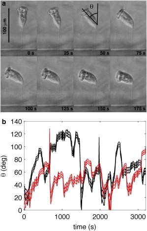
(a) Photos of a single Vorticella convallaria taken from a time-lapse video (see Movie S1 in the Supporting Material). The cilia are attached to a ring at the upper end of the cell body and push fluid parallel to the long axis of the cell body. Note that in the first frame (0 s), the organism is oriented so that it pushes fluid perpendicular to the surface of attachment (the darker area below the organism), and that the organism’s orientation to the substrate changes with time. (b) Plot of the angle of the Vorticella body to the vertical, θ, as a function of time. (Middle lines) θ, whereas the outer lines and shading are the error on θ. (Black lines) From video of Vorticella in culture fluid with nutrients; (gray line/red online) from video of Vorticella in culture fluid without nutrients. Black lines correspond to the images in panel a with a time offset: t = 0 s in panel a corresponds to t = 110 s in panel b. To see this figure in color, go online.
To determine if angled feeding could be a strategy to increase nutrient uptake, we first use a torque calculation to show that experimental observations of living Vorticella feeding at an angle are likely due to active behavior and are not a passive hydrodynamic response to the flow. We then calculate the total flux of food particles or dissolved nutrients as a function of time and feeding angle for model suspension feeders near a planar boundary. We find that model suspension feeders can greatly increase their nutrient uptake by feeding at an angle to the surface, even for nutrients that can diffuse.
Materials and Methods
Vorticella body angle observations
V. convallaria were cultured as described by Nagai et al. (30) until a few organisms, isolated from each other, were observed attached to the thin edge of a cover glass of thickness 145 ± 25 μm. The cover glass with the attached organisms was sandwiched between two clean cover glasses, and placed in a petri dish filled with either culture fluid or with mineral water without nutrients. A single organism was then observed using an Eclipse TE 2000-U inverted microscope (Nikon, Melville, NY) at 10× magnification, recording at 1 frame per s. Two organisms were observed in this way—one in the presence of culture fluid (with nutrients) and one in mineral water (without nutrients). The effective length of the body axis and the angle that the body makes with the vertical, θ, were determined manually for every 10th frame. From these measurements, we extract both θ and also ϕ, the angle the body axis is rotated in or out of the plane of view as a function of time. The results for θ are shown in Fig. 1 b.
Force of Vorticella
Lower and upper bounds for the force on the fluid generated by a feeding V. convallaria were determined using flow field data from experiments (28) and also a V. convallaria observed in the swimming phase of its life. The experimentally measured flow field for an organism squeezed between two slides with no other boundaries nearby was compared to the calculated flow field for a stokeslet between two parallel no-slip boundaries (described in further detail in Pepper et al. (28) Appendix A) and the stokeslet force that resulted in the best match between the two flow fields was determined using least-square fitting. The stokeslet force was found to be 5 × 10⁻¹¹ N using the flow field from a single representative measurement. Modeled and observed flow fields are shown, respectively, in Figs. 2 a and 5 b in Pepper et al. (28) and reproduced in Fig. S1 in the Supporting Material.
An upper bound of the force generated by a typical V. convallaria was estimated by measuring the swimming speed of a single V. convallaria observed during the swimming portion of its life cycle. This organism was video-taped by chance in the experiments described in Pepper et al. (28). The drag on a spherical object traveling at speed u is F = 6πμau, where μ is the viscosity of water, and a is the radius of the sphere. From the observed swimming speed (u = 400 μm/s), radius (a ≈ 65 μm), and the viscosity of water (μ = 1 × 10⁻³ Pa ⋅ s), we can estimate the force generated by the organism as approximately 5 × 10⁻¹⁰ N. This rough estimate of the force can be considered an upper bound for the force generated by a feeding organism. V. convallaria grow a second band of cilia, which they use for locomotion during the swimming phase of their life (31). These lower and upper bounds for the force generated by V. convallaria match well the force of ∼1 × 10⁻¹¹–1 × 10⁻¹⁰ N generated by Opercularia asymmetrica, a ciliate of similar size to Vorticella (19).
Scaling
Throughout this article we use dimensionless variables. For reference, we list here the scalings used. Lengths are scaled by h, the distance from the stokeslet to the wall. Velocities are scaled by α/(μh), where μ is the viscosity of the fluid, and α is the force the stokeslet exerts on the fluid. Total mass fluxes are scaled by (chα)/μ, where c is the concentration of nutrients in undepleted fluid (or at infinity). Torques are scaled by αh. Times are scaled by (μh2)/α. For Vorticella we approximate h ≈ 100 μm and α ≈ 5 × 10⁻¹¹ −5 × 10⁻¹⁰ N. This approximation gives a velocity scale of approximately 500–5000 μm/s, a total mass flux scale of approximately c × (5–50 nL/s), a torque scale of approximately 5 × 10⁻¹⁴ −5 × 10⁻¹⁵ Nm, and a timescale of ∼0.02−0.2 s.
Torque on a Model Vorticella
Vorticella spp. can change their feeding angle with respect to the substratum (Fig. 1), but is this change a passive response to the feeding flow that the organism generates, or an active behavior on the part of the organism? To answer this question, we calculate the hydrodynamic torque on a model Vorticella from the fluid flow it generates as a function of the organism’s feeding angle. We approximate the feeding flow generated by an individual angled suspension feeder as a point force, or stokeslet, pushing fluid at some angle relative to a flat plane (Fig. 2). A stokeslet is a simple and common model for a suspension feeder (13,19,26,27,29,32): it captures the physical feature that the organism is pushing fluid in a particular direction with a particular force, but does not model the body size or shape of the organism. The stokeslet flow model is described in more detail in Appendix A.
Figure 2.

A schematic of the stokeslet model for Vorticella. (a) Image of a Vorticella convallaria; scale bar is 100 μm. (b) Sketch of a Vorticella showing stalk, cell body, and cilia. Model elements are overlaid. (c) Stokeslet model for a Vorticella. The stokeslet is a point force at the origin of the arrow (red online) at a distance h from the no-slip boundary (indicated by a thick line). The arrow points in the direction in which the stokeslet forces the fluid at an angle θ from the vertical. (Dashed line) The feeding disk, radius rd. In the image in panel a, h ≈ 100 μm and rd ≈ 15 μm. To see this figure in color, go online.
With the flow field determined by the stokeslet flow model, the torque on the organism is calculated by approximating the body of the Vorticella as a prolate ellipsoid of revolution centered on the stokeslet (see inset in Fig. 3 for the geometry). Here the stokeslet image system (see Eq. 7) plays the role of an external flow field and so, depending on the orientation of the stokeslet, may produce a torque on the ellipsoid. The torque on this ellipsoid due to an external flow field is
| (1) |
where a is the length of the semimajor axis of the ellipse, d is a unit vector that points along the semimajor axis of the ellipse,
is the vorticity,
is the rate of strain tensor, and u∞ is the external flow undisturbed by the ellipsoid and evaluated at the location of the center of the ellipsoid (33). Here XC, YC, and YH are scalar resistance functions that depend only on the eccentricity of the ellipse as described in Appendix B. All quantities in Eq. 1 are scaled as described in the Materials and Methods.
Figure 3.
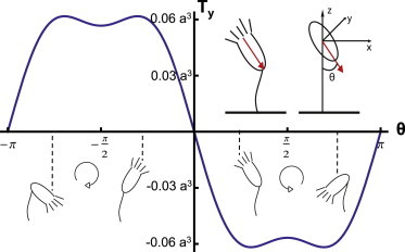
Torque on a model ellipsoid with eccentricity as a function of forcing angle θ. Representative Vorticella body positions are shown for four values of θ. Positive torque points into the page and would result in clockwise rotation. Rotation directions are illustrated using circles with an arrow pointing in the direction of rotation. The torque and a are nondimensionalized as described in the Materials and Methods. In dimensional units, the maximum torque of 0.06a3 is 1.35 × 10⁻¹⁶ Nm if we assume h = 100 μm, that a = 0.3, and that the Vorticella pushes the fluid with a force of 5 × 10⁻¹¹ N. (Inset) This illustration shows our ellipsoid model for Vorticella. The arrow (red online) represents the direction of the stokeslet that generates fluid flow. To see this figure in color, go online.
Without loss of generality, we assume that both the stokeslet and the symmetry axis of the ellipsoid lie in the x-z plane as shown in the inset of Fig. 3. We then find that the torque exerted by the stokeslet flow (see Appendix B) on the body of the organism is
| (2) |
where θ is the angle between the stokeslet and the vertical. This calculation indicates that an upside-down orientation of the Vorticella is stable, as shown in Fig. 3. If the organism tilts at any angle, the hydrodynamic torque pushes it back toward an upside-down orientation (θ = π or −π). This result indicates that the motion documented in Fig. 1 is likely an active behavior on the part of the Vorticella. However, there is a span of time on the left-hand side of the video (see Movie S1 in the Supporting Material) when the Vorticella seems to be stuck in a nearly inverted position, which may be a passive response to hydrodynamic torque. The maximum torque exerted on the organism by the stokeslet flow field is between 0.03 and 0.75% of the torque that the organism could apply at the connection between the body and the stalk using the same force directly (0.03% assumes a = 0.1 and 0.75% assumes a = 0.5; both model the organism as an ellipsoid with eccentricity of 0.6).
We note that the Vorticella in Fig. 1 and Movie S1 are imaged in thin vessels (≈145 μm thick), and that the plane parallel boundaries of the sandwiching cover glasses will quantitatively affect the magnitude of the hydrodynamic torques computed above (28). However, due to symmetry of the parallel-plane geometry, the presence of these walls alone does not give rise to any torque on the organism.
Feeding Without Nutrient Diffusion
To determine if the observed behavior of feeding at an angle is beneficial for nutrient uptake, we use our stokeslet model to determine the total flux of nutrients to the organism. The total flux of nutrients available to the organism is monitored through a feeding disk that represents the area that the organism can reach with its cilia. The feeding disk is in a plane perpendicular to the direction of the stokeslet, and centered on the stokeslet (see Fig. 2), and the model organism feeds by depleting the fluid of nutrients as the fluid passes through this disk. For a typical Vorticella, the cilia sweep out a disk with radius ∼15 μm that is located ∼100 μm away from the substrate of attachment.
A qualitative sense of how turning at an angle can increase nutrient uptake can be seen by looking at representative particle trajectories in the flow for four stokeslet angles (Fig. 4). For the perpendicular stokeslet (Fig. 4 a) all of the fluid particles passing through the feeding disk recirculate, so as the model organism feeds, first the edges of the feeding disk start to see fluid that has completed one turn through the eddy and been depleted of nutrients; as time progresses, more of the feeding disk sees fluid that has passed through before. Eventually, in the absence of diffusion, no fresh fluid is passing through the feeding disk. As the stokeslet angle increases (Fig. 4, b and c), fewer of the streamlines that pass through the feeding disk recirculate, and flux is more stable with time. At some angle, which will depend on the size of the feeding disk, none of the feeding streamlines that pass through the disk recirculate, and we expect the flux of nutrients will not decrease with time. We note that the absence of eddies in the flow for the case of a stokeslet parallel to a plane boundary (Fig. 4 d) has been shown previously (25).
Figure 4.
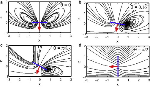
Example fluid particle trajectories for a stokeslet above a plane wall at different angles, θ, shown in the plane of mirror symmetry. The stokeslet direction is represented by an arrow (red online) with origin at the location of the stokeslet (x = y = z = 0). The orientation of the feeding disk is shown as a line (blue online). The size of the line is not representative of the modeled feeding disk size, which for the given distance from stokeslet to wall, would be smaller. The no-slip wall is at z = −1. To see this figure in color, go online.
We model the time dependence of the total flux of nutrients by seeding the feeding disk with a grid of fluid particles and following the trajectories of these nondiffusing particles in time (see Fig. S3). When a particle returns to the disk, the grid to which it returns is no longer receiving nutrients. The total flux of nutrients, Q, is defined as
| (3) |
where u is the velocity field of the fluid and A is the area of the disk. The concentration in this integral, c, depends on the location on the disk, and is either the uniform concentration of nutrients in undepleted fluid (which could include detritus and bacteria), or zero, depending on whether the fluid particle at the relevant grid location has recirculated.
Each square of the grid contributes to the total nutrient flux an amount cℓ2u(xc) ⋅ f, where ℓ is the square-edge length, xc is the position of the point at the center of the grid, and f is a unit vector pointing in the direction of the stokeslet (i.e., orthogonal to the plane of the square). We start a series of fluid particles at the center of each grid and use the known velocity field to follow these fluid particles in time as they move with the fluid surrounding the Vorticella model (see Fig. S3). If at any time a fluid particle returns to the feeding disk, the concentration of nutrients is set to zero in the grid square from which that fluid particle originated, representing complete depletion of nutrients. We assume a uniform concentration of nutrients in the fluid before the Vorticella starts feeding and that when a parcel of fluid passes through the feeding disk, the Vorticella depletes it entirely of useful nutrients.
We keep track of the total nutrient flux through the disk as a function of time after the Vorticella begins feeding, and perform the same calculation for feeding models oriented at various angles to the wall. We choose a stalk length 10 times longer than the Vorticella body radius as in Upadhyaya et al. (34). Because the cilia can reach beyond the body radius we choose a feeding disk of radius rd = 0.15, and break it up into a grid of 1484 elements. We choose this number of elements to balance accuracy and computing time and find that the shape of the curves is only weakly sensitive to grid resolution. Coarser grids overestimate total mass fluxes and the time for the first particle to return to the disk; we choose our grid to match the analytical total mass flux for the perpendicular stokeslet case within 10%. This grid also matches the time for the first particle to return to the disk within 11% for θ = 0.1, and with increasing accuracy at smaller angles, matching the exact result for θ = 0. Our results are qualitatively similar regardless of the specific disk size, as shown in the Supporting Material. We also show in the Supporting Material that the stokeslet model for a Vorticella is very similar with regard to feeding fluxes to a spherical model that takes into account further details of the organism (i.e., body size). To ensure that we end up with a regular grid of points returning and depleting the concentration in each grid square, in our actual algorithm, we measure recirculation time for each grid point by running time backward (35).
Results and Discussion
Overall, the model Vorticella has much greater access to nutrients when at an angle than when perpendicular to a wall (Fig. 5). We find that those model organisms that feed at an angle begin with a slightly higher total flux of nutrients, that this flux dies off more slowly in time, and that the overall decrease in total nutrient flux is less than for perpendicular feeders. For sufficiently large angles, the total nutrient flux remains constant in time and there is no recirculation of fluid through the feeding disk. The total nutrient flux at long times (the right side of Fig. 5) for the parallel stokeslet is approximately six times that for the perpendicular orientation, indicating a large benefit (>500%) from feeding at an angle due to reducing the recirculation in the flow. This long time point is set by the duration of our simulation; if the simulations were run for a longer time, the total nutrient flux for the perpendicular case would decrease even further, eventually going to zero as time goes to infinity. Although the benefit at long times of around 500% comes from an artificial time point, steady-state calculations that include diffusion (done in the following section) show a similar benefit for consumption of nonmotile bacteria.
Figure 5.
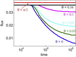
Decrease in total nutrient flux with time for different feeding angles. Different lines (color online) represent model organisms feeding at different angles from the vertical. Times and total nutrient fluxes are nondimensionalized as described in the Materials and Methods. For Vorticella the timescale is ∼0.02–0.2 s. To see this figure in color, go online.
Feeding at an angle also increases nutrient uptake by reducing the effect of viscous drag from the surface, increasing the overall speed of fluid flow and the flow of fluid through the feeding disk. The effect occurs regardless of nutrient depletion, and does not change in time; thus we can determine its contribution to the overall benefit by looking at early time points before the fluid has recirculated through the feeding disk and before nutrients have been depleted. The total nutrient flux at the start time (the left side of Fig. 5) is 1.06 times more for the parallel stokeslet than the perpendicular stokeslet, indicating that there is a small benefit (∼6%) from feeding at an angle due to reducing viscous drag and increasing the fluid velocity and net flow of fluid through the feeding disk. This small benefit matches earlier predictions (13), and shows that as feeding time increases and the organism could begin to see recirculated fluid, the primary benefit to feeding at an angle comes from reduced recirculation. The total nutrient flux at the start time can also be thought of as the clearance velocity averaged over the feeding disk, a common experimental measure to determine how much water is filtered by such organisms (5,16). Clearance velocity is only ∼6% different between the parallel and perpendicular orientations and actual nutrient uptake at long times is >500% different due to the decrease of total nutrient flux. Because fluid recirculates through the disk for the perpendicular feeder, estimates of clearance velocities made using measured fluid velocities near organisms without taking into account the effect of recirculation may significantly overestimate the amount of water cleared by these organisms if the organisms spend time feeding in a near-perpendicular orientation.
Even in cases of recirculation, the total nutrient flux does not start to decrease until the smallest closed eddy that intersects the disk has turned over once, which is why the decay in this flux reported in Fig. 5 only begins at times greater than (104). Using a feeding force and model dimensions appropriate for sessile suspension feeders, the time for this turnover is 2 min to 9 h. The large time range results from the range of estimates for the forces generated by these organisms, and the range of the ratio of body size to stalk length between individual organisms in a species. For example, we estimate that for Vorticella, the turnover time ranges from 20 min to 6 h (h = 100 μm, rd = 0.15, α = 5 × 10⁻¹⁰–5 × 10⁻¹¹ N); for choanoflagellates, the range is 6 min to 3 h (h = 10–20 μm, rd = 0.25–0.15, α = 2.4 × 10⁻¹² N (36)); and for P. vestida, the range is 2 min to 9 h (h = 10–30 μm, rd = 0.25–0.1, α = 10 × 10−11 N (5)). We find that the time for the smallest eddy to recirculate decreases for larger ratios of feeding disk radius to stalk length as rd−4 (Fig. 6); see the Supporting Material for more information. Larger feeding disks intersect more of the feeding eddy, so have shorter recirculation time.
Figure 6.
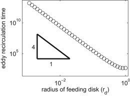
Eddy recirculation time as a function of rd, the radius of the feeding disk scaled by h. For this calculation the stokeslet is forcing fluid perpendicular to the boundary, θ = 0. Start positions are all in a plane that includes the stokeslet and is parallel to the boundary, and time is scaled as described in the Materials and Methods.
Feeding Including Nutrient Diffusion
The times for the smallest eddy to recirculate are relatively long, and we might expect diffusion of nutrients across streamlines to replenish the depleted eddies. We therefore include a second model, which includes diffusion of nutrients. In this model, the suspension feeder is again modeled as a stokeslet above a boundary, but instead of following fluid particles in time, we numerically calculate the steady-state concentration of food particles or dissolved nutrients in a large simulation domain surrounding the organism. The total flux of food particles or nutrients is calculated over a sphere surrounding the model organism.
Again modeling the organism as a stokeslet pointing at some angle above a plane boundary, we solve for the steady-state concentration of diffusing nutrients using the advection diffusion equation
| (4) |
where u is the fluid velocity, and c is the concentration of nutrients or food particles in the fluid. The equation is scaled as described in the Materials and Methods. With those scalings, Pe = α/μD, where α is the stokeslet force, μ is the viscosity of the fluid, and D is the diffusion constant of the nutrient or food particle being consumed.
We solve for c in a box above the plane boundary using finite-element analysis with the software COMSOL MULTIPHYSICS (COMSOL, Palo Alto, CA) (see Fig. S2). We enforce no flux across the symmetry plane and on the substrate boundary, and set c = 1 on the other four faces of the box. Additionally, we set c = 0 on a spherical capture surface surrounding the stokeslet. The total flux of nutrients across this sphere is calculated using a Lagrange multiplier to determine feeding success as a function of stokeslet angle. To achieve true first-order accuracy in our flux computations, we extracted the flux from the Lagrange multiplier used by COMSOL to enforce the c = 0 condition on the spherical capture surface. We use a feeding sphere of radius rs = 0.1, which is slightly different than the feeding disk, rd = 0.15, used in our model without diffusion. The total simulation has 162,501 P1 elements, including 232 elements on the boundary of the sphere. We choose a feeding sphere in this simulation rather than the feeding disk used in the no-diffusion case for computational ease, but we do not expect this modest difference between models to affect our qualitative conclusions.
The size of the simulation box is set such that the effect of the chamber size on the total flux of nutrients to the organism was <1%. The resulting dimensions were for the height of the box (distance between the plane boundary and the boundary above it), and for the length and width of the box (see Fig. S2).
Results and Discussion
In our advection-diffusion model, the relative importance of advective transport of nutrients to diffusive transport is captured by the Péclet number, Pe = LU/D, where L is a typical length scale of the flow, U is a typical velocity, and D is the diffusion coefficient of the nutrient or prey particle of interest. Large Pe indicates that effects from diffusion are small. For feeding Vorticella, the Péclet number for nonmotile bacteria ranges from 103 to 105. Consistent with earlier definitions, we choose L=h, and U=α/8πμh. This range for Pe assumes bacteria diffuse as spheres of the appropriate size (0.1–10 μm) and the diffusion constant is calculated using the Stokes-Einstein relation (37), yielding D = 2 × 10⁻¹² m2/s and D = 2 × 10⁻¹⁴ m2/s for 0.1 μm and 10 μm spheres, respectively. For motile bacteria and small diffusing nutrient molecules, D ≈ 10−10 m2/s (37), yielding Pe = (10). With these scales in mind, our simulations shows that for Vorticella feeding on nonmotile bacteria, feeding at an angle to the substratum is beneficial (Fig. 7). At Pe = 103, the model organism can access about 4 times more nutrients when feeding parallel to the substratum than when feeding perpendicular. However, Fig. 7 also shows that for food sources that diffuse more quickly, such as motile bacteria and dissolved molecules, diffusion dominates, and the model suspension feeder no longer derives significant benefit from feeding at an angle. Note that even in the regime of high Péclet number, where we expect nutrient transport to be dominated by advection (i.e., flow generated by the organism), a small amount of diffusion is necessary to provide any steady-state nutrient flux to organisms feeding perpendicular to the substrate.
Figure 7.
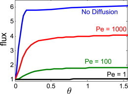
Steady-state feeding flux as a function of feeding angle, θ, measured from the vertical. Total nutrient flux is normalized by the total nutrient flux at θ = 0 for each case. The No-Diffusion case is taken from the final time point in Fig. 5. To see this figure in color, go online.
One of the most abundant photosynthetic organisms on earth, Procholorococcus, is a nonmotile bacteria that lives in the ocean and has a diameter of ∼0.5 μm (38). These abundant organisms would therefore have a Péclet number of around 2 × 10³ in the Vorticella’s feeding flow. Procholorococcus are particularly dominant in nutrient-poor environments, where sessile suspension feeders might have few other sources of nutrients (38). Overall, our advection-diffusion model shows that feeding at an angle is beneficial for some plentiful food sources for Vorticella, so is likely a good strategy for these organisms to access the maximum amount of food. It also indicates that when estimating the amount of fluid such organisms clear in a given time, both the typical orientation of the organism relative to the substratum and the diffusivity of the food or contaminant of interest should be taken in to account for more accurate results.
Discussion
It is important to note that, given the slow timescale for the eddy to turn over, the benefits of feeding at an angle are likely most important in environments with very slow to no external flow, such as ponds, puddles, and protected areas with dense vegetation. These are all common habitats for sessile suspension feeders, and there is some evidence that these organisms may be more abundant in areas of slower flow (39).
Additionally, in our calculations and experiments we treat a single Vorticella above a flat wall. However, in nature, the situation could be quite different. The Vorticella could have nearby neighbors feeding in a similar manner; it could be confined by other nearby surfaces; or could be on a surface that is not locally flat. All of these situations would affect the flux of nutrients that the feeding organism can access, and provide interesting avenues for further study.
We have studied feeding in an idealized situation where nutrients are distributed homogeneously. Real filter feeders live in spatially patchy and temporally fluctuating environments, raising the possibility that feeding angle may be actively modulated similar to locomotory infotaxis strategies (40,41). Indeed, we observed that, in addition to varying the polar feeding angle, θ, Vorticella also vary the azimuthal angle, ϕ. This rotation would make sense as an active behavior to consume nutrient sources from all directions around the organism. Preliminary results taken from the video available in the Supporting Material give a correlation time for the rotation of ∼2 min for the Vorticella that has access to nutrients in the culture fluid, and ∼5 min for the one that has no access to nutrients. Although shorter than the typical eddy turnover time, these times are reasonable for increasing nutrient uptake. Future studies could determine if this rotation time is optimized for nutrient uptake, and if it is consistent among a population of organisms, between different species, or between the same organisms in different geometries.
Conclusion
Observations of living Vorticella show that they feed at an angle to the surfaces to which they are attached. Our calculations show that the hydrodynamic forces on a simple model organism stabilize it in a vertical orientation, so changes in orientation angle for living Vorticella are likely the result of active behavior. We show that, by feeding at an angle, organisms solve the problem of eddies that arise from forcing fluid near a boundary. We further show that angled feeding increases nutrient uptake for several model organisms feeding on biologically relevant food with slow diffusion, such as nonmotile bacteria. For other nutrients that diffuse more rapidly, such as small molecules, feeding at an angle is only slightly favored.
Our work resolves an open question of how attached suspension-feeding organisms escape physical limitations associated with feeding near surfaces. These data also reveal the high degree of sensitivity of clearance rates (e.g., of bacteria and potentially of contaminants like oil contained in the bacteria) to organism behavior and hydrodynamic constraints on their feeding. Estimates of clearance velocities made using measured fluid velocities near organisms without taking into account the effect of recirculation may significantly overestimate the amount of water cleared by these organisms. We anticipate that our results will also be a starting point for exploring optimization strategies that sessile microorganisms can employ to feed on different prey types and in heterogeneous environments.
Acknowledgments
We thank Paul Matsudaira for help with experiments used to determine the force on the fluid generated by Vorticella and Wesley Lee for help measuring Vorticella body lengths and angles from videos.
We also thank the National Science Foundation and Harvard Materials Research Science & Engineering Center (under grant No. DMR-0820484) for support of this project. This research was partially funded by the National Science Foundation under Integrative Graduate Education and Research Traineeship grant No. DGE-0221682. R.E.P. is supported by the Miller Institute for Basic Research in Science at the University of California, Berkeley. M.R. gratefully acknowledges financial support from the Alfred P. Sloan Foundation.
Appendix A: Stokeslet Above a Plane Boundary
We solve for the velocity, u, for a stokeslet a distance h above a plane no-slip wall exerting a force α on the surrounding fluid and pointing in direction f = (fx, fy, fz) where f is a unit vector. For low Re flow, we satisfy the Stokes equation and continuity equation
| (5) |
where x0 is the position of the stokeslet, and where we have scaled all lengths by h, velocities by α/(μh), and stresses by α/h2 where μ is the viscosity of the fluid. The solution for a stokeslet at an angle above a no-slip boundary is well known to be the solution for a stokeslet in free space plus an image system consisting of a stokeslet, a source dipole, and a stokeslet doublet (42–44). The velocity is given by a Green’s function solution (44)
| (6) |
where x0 is the position of the stokeslet, with
| (7) |
where we define position relative to the stokeslet, xs = x – x0, with x0 = (0,0,1) and position relative to the image, xim = x − x0im, where x0im = (0,0,−1). The components of the above equation are the stokeslet term,
| (8) |
where r = |x|; the image stokeslet term, GS(xim); the dipole term,
| (9) |
where fim = (fx, fy, −fz); and finally the stokeslet doublet term,
| (10) |
where x = (x, y, z) (44). We note that while we use the same notation as Pozrikidis (44), our Green’s functions are vectors rather than tensors, and we have introduced the vector fim to simplify sign conventions.
Appendix B: Torque on an Ellipsoid in a Stokeslet Flow Field
Here we calculate the torque on an prolate ellipsoid of revolution with semimajor axis length a and semiminor axis length b centered on a stokeslet above a plane boundary. The unit vector along the symmetry axis of the ellipse, d, and the direction of the stokeslet force, f, point in the same direction. Kim and Karrila (33) use a singularity representation to solve for the hydrodynamic force, torque, and stresslet exerted by the fluid on a moving prolate spheroid. If the fluid has an undisturbed velocity u∞, the torque is given by
| (11) |
where
is the vorticity, ω is the rotational velocity of the ellipse, and
is the rate of strain tensor, and where the velocity is evaluated at the center of the ellipse (33). The resistance functions depend on the eccentricity of the ellipse,
and are given by
| (12a) |
| (12b) |
| (12c) |
| (12d) |
For a stationary ellipsoid, ω = 0, and Eq. 11 simplifies to Eq. 1 in the main text if lengths are scaled by h, velocities are scaled by α(μh), and torques are scaled by αh, where α is a representative force scale (i.e., the strength of the stokeslet if u∞ is the flow field of a stokeslet). Here the stokeslet image system (see Eq. 7) plays the role of an external flow field and so, depending on the orientation of the stokeslet, may produce a torque on the ellipsoid.
Supporting Material
References
- 1.Laybourn J. Energy budgets for Stentor coeruleus Ehrenberg (Ciliophora) Oecologia. 1976;22:431–437. doi: 10.1007/BF00345319. [DOI] [PubMed] [Google Scholar]
- 2.Kankaala P., Eloranta P. Epizooic ciliates (Vorticella sp.) compete for food with their host Daphnia longispina in a small polyhumic lake. Oecologia. 1987;73:203–206. doi: 10.1007/BF00377508. [DOI] [PubMed] [Google Scholar]
- 3.Fenchel T. Ecology of heterotropic microflagellates. IV. Quantitative occurrence and importance as bacterial consumers. Mar. Ecol. Prog. Ser. 1982;9:35–42. [Google Scholar]
- 4.Sherr E., Sherr B. Role of microbes in pelagic food webs: a revised concept. Limnol. Oceanogr. 1988;33:1225–1227. [Google Scholar]
- 5.Christensen-Dalsgaard K.K., Fenchel T. Increased filtration efficiency of attached compared to free-swimming flagellates. Aquat. Microb. Ecol. 2003;33:77–86. [Google Scholar]
- 6.King N. Choanoflagellates. Curr. Biol. 2005;15:R113–R114. doi: 10.1016/j.cub.2005.02.004. [DOI] [PubMed] [Google Scholar]
- 7.Reid R. Fluctuations in populations of three Vorticella species from an activated-sludge sewage plant. J. Protozool. 1969;16:103–111. doi: 10.1111/j.1550-7408.1969.tb02240.x. [DOI] [PubMed] [Google Scholar]
- 8.Chen S., Xu M., Shao Y. The activated-sludge fauna and performance of five sewage treatment plants in Beijing, China. Eur. J. Protistol. 2004;40:147–152. [Google Scholar]
- 9.McCauley R.N. The biological effects of oil pollution in a river. Limnol. Oceanogr. 1966;11:475–486. [Google Scholar]
- 10.Andrews A.R., Floodgate G.D. Some observations on the interactions of marine protozoa and crude oil residues. Mar. Biol. 1974;25:7–12. [Google Scholar]
- 11.Scott B.F., Wade P.J., Taylor W.D. Impact of oil and oil-dispersant mixtures on the fauna of freshwater ponds. Sci. Total Environ. 1984;35:191–206. doi: 10.1016/0048-9697(84)90062-7. [DOI] [PubMed] [Google Scholar]
- 12.Gertler C., Näther D.J., Golyshin P.N. A mesocosm study of the changes in marine flagellate and ciliate communities in a crude oil bioremediation trial. Microb. Ecol. 2010;60:180–191. doi: 10.1007/s00248-010-9660-3. [DOI] [PubMed] [Google Scholar]
- 13.Fenchel T. Protozoan filter feeding. Prog. Protistol. 1986;2:65–113. [Google Scholar]
- 14.Leadbeater B.S.C., Green J.C. CRC Press; Boca Raton, FL: 2000. Flagellates: Unity, Diversity and Evolution, Vol. 59. [Google Scholar]
- 15.Fenchel T. Springer-Verlag; New York: 1987. Ecology of Protozoa: The Biology of Free-Living Phagotrophic Protists. [Google Scholar]
- 16.Boenigk J., Arndt H. Particle handling during interception feeding by four species of heterotrophic nanoflagellates. J. Eukaryot. Microbiol. 2000;47:350–358. doi: 10.1111/j.1550-7408.2000.tb00060.x. [DOI] [PubMed] [Google Scholar]
- 17.Boenigk J., Arndt H. Bacterivory by heterotrophic flagellates: community structure and feeding strategies. Antonie van Leeuwenhoek. 2002;81:465–480. doi: 10.1023/a:1020509305868. [DOI] [PubMed] [Google Scholar]
- 18.Rapport D.J., Berger J., Reid D.B.W. Determination of food preference of Stentor coeruleus. Biol. Bull. 1972;142:103–109. [Google Scholar]
- 19.Hartmann C., Ozmutlu O., Delgado A. Analysis of the flow field induced by the sessile peritrichous ciliate Opercularia asymmetrica. J. Biomech. 2007;40:137–148. doi: 10.1016/j.jbiomech.2005.11.006. [DOI] [PubMed] [Google Scholar]
- 20.Sleigh M.A., Barlow D. Collection of food by Vorticella. Trans. Am. Microsc. Soc. 1976;95:482–486. [Google Scholar]
- 21.Rubenstein D., Koehl M.A.R. The mechanisms of filter feeding: some theoretical considerations. Am. Nat. 1977;111:981–994. [Google Scholar]
- 22.Labarbera M. Feeding currents and particle capture mechanisms in suspension feeding animals. Am. Zool. 1984;24:71–84. [Google Scholar]
- 23.Vogel S. 2nd Ed. Princeton University Press; Princeton, NJ: 1996. Life in Moving Fluids. [Google Scholar]
- 24.Lighthill J. Flagellar hydrodynamics. SIAM Rev. 1976;18:161–230. [Google Scholar]
- 25.Liron N., Blake J.R. Existence of viscous eddies near boundaries. J. Fluid Mech. 1981;107:109–129. [Google Scholar]
- 26.Blake J.R., Otto S.R. Ciliary propulsion, chaotic filtration and a ‘blinking’ stokeslet. J. Eng. Math. 1996;30:151–168. [Google Scholar]
- 27.Blake J.R., Otto S.R., Blake D.A. Filter feeding, chaotic filtration, and a blinking Stokeslet. Theor. Comput. Fluid Dyn. 1998;10:23–36. [Google Scholar]
- 28.Pepper R.E., Roper M., Stone H.A. Nearby boundaries create eddies near microscopic filter feeders. J. R. Soc. Interface. 2010;7:851–862. doi: 10.1098/rsif.2009.0419. [DOI] [PMC free article] [PubMed] [Google Scholar]
- 29.Pettitt M.E., Orme B.A.A., Leadbeater B.S.C. The hydrodynamics of filter feeding in choanoflagellates. Eur. J. Protistol. 2002;38:313–332. [Google Scholar]
- 30.Nagai M., Oishi M.I., Fujita H. Three-dimensional two-component velocity measurement of the flow field induced by the Vorticella picta microorganism using a confocal microparticle image velocimetry technique. Biomicrofluidics. 2009;3:14105. doi: 10.1063/1.3105106. [DOI] [PMC free article] [PubMed] [Google Scholar]
- 31.Vacchiano E., Dreisbach A., Buhse H.E. Morphogenetic transitions and cytoskeletal elements of the stalked zooid and the telotroch stages in the peritrich ciliate Vorticella convallaria. J. Eukaryot. Microbiol. 1992;39:101–106. [Google Scholar]
- 32.Drescher K., Leptos K.C., Goldstein R.E. Dancing volvox: hydrodynamic bound states of swimming algae. Phys. Rev. Lett. 2009;102:168101–168104. doi: 10.1103/PhysRevLett.102.168101. [DOI] [PMC free article] [PubMed] [Google Scholar]
- 33.Kim S., Karrila S.J. Dover Publications; Mineola, NY: 2005. Microhydrodynamics: Principles and Selected Applications. [Google Scholar]
- 34.Upadhyaya A., Baraban M., Mahadevan L. Power-limited contraction dynamics of Vorticella convallaria: an ultrafast biological spring. Biophys. J. 2008;94:265–272. doi: 10.1529/biophysj.107.108852. [DOI] [PMC free article] [PubMed] [Google Scholar]
- 35.Stone Z.B., Stone H.A. Imaging and quantifying mixing in a model droplet micromixer. Phys. Fluids. 2005;17:063103–063111. [Google Scholar]
- 36.Roper M., Dayel M.J., Koehl M.A.R. Cooperatively generated stresslet flows supply fresh fluid to multicellular choanoflagellate colonies. Phys. Rev. Lett. 2013;110:228104. doi: 10.1103/PhysRevLett.110.228104. [DOI] [PubMed] [Google Scholar]
- 37.Berg H.C. Princeton University Press; Princeton, NJ: 1993. Random Walks in Biology. [Google Scholar]
- 38.Partensky F., Hess W.R., Vaulot D. Prochlorococcus, a marine photosynthetic prokaryote of global significance. Microbiol. Mol. Biol. Rev. 1999;63:106–127. doi: 10.1128/mmbr.63.1.106-127.1999. [DOI] [PMC free article] [PubMed] [Google Scholar]
- 39.Silvester N.R., Sleigh M.A. The forces on microorganisms at surfaces in flowing water. Freshw. Biol. 1985;15:433–448. [Google Scholar]
- 40.Vergassola M., Villermaux E., Shraiman B.I. ‘Infotaxis’ as a strategy for searching without gradients. Nature. 2007;445:406–409. doi: 10.1038/nature05464. [DOI] [PubMed] [Google Scholar]
- 41.Stocker R. Marine microbes see a sea of gradients. Science. 2012;338:628–633. doi: 10.1126/science.1208929. [DOI] [PubMed] [Google Scholar]
- 42.Blake J.R. A note on the image system for a stokeslet in a no-slip boundary. Math. Proc. Camb. Philos. Soc. 1971;70:303–310. [Google Scholar]
- 43.Blake J.R., Chwang A. Fundamental singularities of viscous flow. J. Eng. Math. 1974;8:23–29. [Google Scholar]
- 44.Pozrikidis C. Cambridge University Press; New York: 1992. Boundary Integral and Singularity Methods for Linearized Viscous Flow. [Google Scholar]
- 45.Noland L.E., Finley H.E. Studies on the taxonomy of the genus Vorticella. Trans. Am. Microsc. Soc. 1931;50:81–123. [Google Scholar]
Associated Data
This section collects any data citations, data availability statements, or supplementary materials included in this article.