Abstract
As the ability to measure dense genetic markers approaches the limit of the DNA sequence itself, taking advantage of possible clustering of genetic variants in, and around, a gene would benefit genetic association analyses, and likely provide biological insights. The greatest benefit might be realized when multiple rare variants cluster in a functional region. Several statistical tests have been developed, one of which is based on the popular Kulldorff scan statistic for spatial clustering of disease. We extended another popular spatial clustering method – Tango’s statistic – to genomic sequence data. An advantage of Tango’s method is that it is rapid to compute, and when single test statistic is computed, its distribution is well approximated by a scaled chi-square distribution, making computation of p-values very rapid. We compared the Type-I error rates and power of several clustering statistics, as well as the omnibus sequence kernel association test (SKAT). Although our version of Tango’s statistic, which we call “Kernel Distance” statistic, took approximately half the time to compute than the Kulldorff scan statistic, it had slightly less power than the scan statistic. Our results showed that the Ionita-Laza version of Kulldorff’s scan statistic had the greatest power over a range of clustering scenarios.
Keywords: genetic association, kernel distance, SKAT statistic
Introduction
Genomic technologies, such as whole exome sequencing, or whole genome sequencing, provide rich resources to screen for genetic variants associated with complex diseases. Although a number of statistical methods have been developed to screen genomes for individual variants, or groups of variants, for their association with disease, only a few have focused specifically on detecting clusters of variants that occur more frequently among cases than controls. General omnibus statistics, such as sequence kernel association tests (SKAT) [Kwee, et al. 2008; Lee, et al. 2012a; Lee, et al. 2012b; Wu, et al. 2011] or burden-type tests [Asimit and Zeggini 2010; Bansal, et al. 2010; Basu and Pan 2010], might not be as powerful as statistics designed to be sensitive to tight clustering of risk variants within small genomic regions. Two recently proposed statistics were developed for detecting clusters of variants. Ionita-Laza et al. [Ionita-Laza, et al. 2012] extended Kulldorff’s likelihood ratio scan statistic [Kulldorff 2007], developed for detecting spatial clusters of disease to scan for clusters of risk variants along a genomic region. Intuitively, this method computes a likelihood ratio statistic to compare the frequency of variants carried among cases and controls within a genomic window vs. those frequencies outside of a genomic window, and scans the genomic region of interest by sliding the window along the genome while evaluating a range of window sizes. Fier et al. [Fier, et al. 2012] also developed a method based on spatial clustering, emphasizing physical distances between variants. They combined physical distances between variants with minor allele frequencies of the variants to create weighted distances between variants, to then compare the distributions of these measures between cases and controls using the nonparametric Ansari-Bradley statistic, which is sensitive to differences in scale of the two distributions. As emphasized by Fier et al., a number of biological features of genes support the view that risk variants might cluster in restricted regions: 1) protein domains tend to have similar function, and variants within the same domain can be located in close proximity on the DNA sequence; 2) multiple variants in a gene regulatory element can be physically clustered.
Spatial clustering of disease in geographic regions, as well as temporal clustering, have been a topic of interest in epidemiologic studies for decades, leading to many competing statistical methods [Tango 2010]. Two major competitors have been Kulldorff’s scan statistic, extended by Ionita-Laza et al. [Ionita-Laza, et al. 2012] to genomic scans, and Tango’s kernel statistic. In spatial clustering of disease, Tango’s kernel method computes all pair-wise geographic distances between diseased cases and compares theses distances with those computed from controls.
To appreciate the approach by Tango, a few insights from spatial statistics and geographical clustering of disease are useful. This approach requires computing pairwise geographic distances between all pairs of subjects, and then compares the distribution of pairwise distances between cases vs. controls. If a cluster of diseased cases exists, however, the average pairwise distances among them can be drowned out by the many pairs of random large distances. For this reason, Mantel [Mantel 1967] and others have suggested truncating larger distances, say more than a few miles. Alternatively, Tango [Tango 1984] used a nonlinear metric of distance that decreases more rapidly than linear.For example, let dij denote the linear distance between subjects i and j. One of Tango’s metrics is Aij(τ)= e−|dij|/τ, where τ is a scale parameter and interpreted as a measure of cluster size, equal to the maximum distance between cases; cases further apart cannot be considered to be in the same cluster. Large values of τ will be sensitive to a large cluster, and a small value of τ to a small cluster. The problem is choosing τ, because we do not know the number of clusters, nor their sizes. To get around this, Tango [Tango 2000] later proposed a different metric, Aij(τ)=e−4(dij/τ)2, and allowed τ to vary, essentially a scan statistic, and used the minimum p-value as the test statistic, with simulations to compute an adjusted global p-value. For case-control data, Tango’s statistic is a quadratic statistic, Q = (O−E)′A(O − E), where O is the vector of counts of cases at different points, E is the null expected vector of variant counts among cases (determined by total counts among cases + controls). Because Tango’s method can be expressed as a quadratic kernel statistic, much like the SKAT statistic, it is appealing for genomic scans because it can be rapidly computed. Furthermore, it offers a kernel-smoothing way to plot the distribution of variants, to graphically view potential clustering of variants. For these reasons, we extend Tango’s ideas to methods useful to scan genomic regions for variant clustering.
In the following section we develop a kernel statistic for scanning genomic regions for excessive clustering of variants among cases relative to controls. We then used simulations to compare a number of statistical methods for their Type-I error rates and power to detect one or more clusters, including the scan statistic of Ionita-Laza, the spatial clustering method of Fier et al., our proposed kernel statistic, and the omnibus SKAT statistic. Based on these simulation results, we make recommendations on analytic strategies to detect clusters of risk variants.
Methods
Kernel Distance Clustering
Because methods for detecting clustering of variants are based on measures of distances among variants, or the frequency of variants within a window, only subjects that carry at least one minor allele from at least one of the possible variant sites are included in analyses (i.e., subjects that are homozygous for common alleles across all variant positions in the region of interest are excluded). To develop a kernel statistic, it is helpful to label each minor allele as originating from a case versus control, and then cross-classify the variants according to disease status and their positions, as in the 2 ×m contingency table depicted in Table 1. Note that row totals rd and rc are the number of variants among cases and controls, respectively, and that the column total Cj is the total number of variants at position j. Conditional on row totals, the vector of variant frequencies among cases is pd = a/rd, and among controls, pc = b/rc. The vector of differences in variant frequencies is δ = pd − pc; it is this vector that captures information on the relative clustering of variants between cases and controls. Although we base our derivations on δ = pd − pc, it can be shown that this is the same as Tango’s approach, because δ = (O − E)N/rdrc, where O is the vector of variant counts for cases (vector a in Table 1), and E is the null expected vector of counts based on the contingency table of Table 1.
Table 1.
Cross-classification of case-control status of genetic markers at m positions.
| 1 | 2 | … | m | Total | |
|---|---|---|---|---|---|
|
|
|||||
| cases | a 1 | a 2 | am | rd | |
|
|
|||||
| controls | b 1 | b 2 | bm | rc | |
|
|
|||||
| Total | c 1 | c 2 | cm | N | |
For clustering, we wish to use a kernel matrix, A, that measures distances between pairs of variant positions, and then use the kernel matrix to create the quadratic statistic Q δ′ Aδ. Note that Q = ΣiΣjδiδjAij, so this statistic measures how the covariation of the differential of variant frequencies at different positions depends on the distance of the positions, with distance determined by the kernel Aij. To compute p-values, one could use moments of Q to obtain a scaled chi-square distribution [Tango 2010], or use Davies’ method [Wu, et al. 2011], but we expect that permutation-based p-values (permuting case-control status) will be more accurate for rare variants, especially if they are not in linkage equilibrium. When using multiple kernel matrices, as we discuss below with different scaling factors, and taking the maximum statistic over all tests as the global statistic, permutation p-values are required. Also, the above quadratic statistic is two-sided, in the sense that the direction of δj can be either positive (cases having a higher frequency of variants than controls) or negative (cases having a lower frequency of variants than controls). A one-sided version, favoring only cases having a greater frequency of variants than controls, can be calculated by truncating δj to 0 if δj < 0.
A subtle side benefit of the kernel method is that if the null hypothesis is rejected, the kernel matrix can be used as a smoother to create a plot of where the most likely clusters occur. That is, matrix A serves as a smoother, like in semi-parametric regression [Ruppert, et al. 2005], so that a smoothed fitted value can be computed, , and then plotted versus chromosome position.
Choice of Kernels
The kernel function determines how rapid similarity decreases to 0 as the distance d increases. Figure 1 illustrates commonly used kernel functions for density estimation. The Gaussian radial basis function (right panel of figure), K(u) = exp(−u2/τ), is the form used in Tango’s statistic. Because the scaling factor τ is unknown, Tango computed the quadratic statistic over a range of values, and used the maximum statistic. Figure 1 illustrates that the tri-weight function (light blue broken line), has similar shape as a Gaussian function with similar scaled distance. For this reason, we used the tri-weight function over a range of scaled distances. That is, we scaled the distance based on a user-specified maximum distance. For example, to scale distances to the range −1 to +1, we used dscaled = d/maxd, where maxd is a user-specified maximum distance of interest,perhaps maxd = 10kb. We then evaluated the kernel statistic at increments of 10% of the maximum (i.e., 10%, 20%, …, 100%), and took the maximum statistic over all 10 values of dscaled. This essentially zooms in to 10% of the maximum, and then outwards up to 100% of the maximum. If only a single value of dscaled were used, the p-value could be well approximated by a scaled chi-square distribution [Tango 2010; Wu, et al. 2011], but we used 1,000 permutations of the phenotype to account for using 10 increments to compute p-values.
Figure 1.
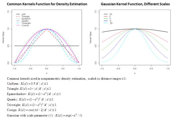
Options for kernel functions.
Our approach for dscaled is a computationally efficient approach that approximates the Gaussian kernel using 10 different scaling factors, τ’s. We refer to the statistic from this method as the “Kernel-Distance” statistic. Beyond the smooth kernel functions illustrated in Figure 1, alternative kernels could be used, such as a threshold (t) for hot-spot detection, aij (d,t) =1 if |d|≤ t (0 otherwise), where the threshold t could vary. This type of hard threshold is similar to Kulldorf’s scan statistic, as Ionita-Laza et al. [Ionita-Laza, et al. 2012] used for scanning for clusters of rare variants.
Adjusting For Covariates
To adjust for categorical covariates, we could follow ideas in Breslow and Day [Breslow and Day 1980]for stratified 2 × m tables, stratified on important covariates. In this situation, we would have a 2 × m table for each stratum, along with vectors as and bs for stratum s. Then the statistic for clustering, adjusted for strata, would be , where we sum over strata to create δ•. This refinement computes the differential of variant frequencies between cases and controls within each stratum, δi, adjusting for the stratum’s effect.
To extend this idea to continuous covariates, and allow subjects to contribute multiple variants to the various positions, we propose using logistic regression on an expanded data set in order to create adjusted expected values. For subject i with ti variants, we create ti replicate records, replicating disease status (yi) and covariate records (xi). For this expanded data set, we use logistic regression to compute fitted values . An example is illustrated in Table 2 for 3 subjects. To compute the sum of residuals at position j, we use . Then the vector of summed residuals, r, is used in the quadratic statistic, Q = r′Ar. This statistic evaluates whether the residuals, after adjusting for covariates, are clustered. This approach might be useful be if one of the positions includes a SNP from GWAS, and the other positions are follow-up fine mapping, and one would want to test the clustering of the fine mapping variants, adjusted for the SNP from GWAS, by using the SNP from GWAS as a covariate.
Table 2.
Example expanded data set for 3 subjects to compute covariate-fitted values,
| Subject | Position | ||||
|---|---|---|---|---|---|
| (i) | (j) | yi | xi | ||
| 1 | 1 | 1 | x 1 | ||
| 1 | 2 | 1 | x 1 |
|
|
|
| |||||
| 2 | 2 | 1 | x 2 |
|
|
| 2 | 3 | 1 | x 2 |
|
|
| 2 | 5 | 1 | x 2 |
|
|
|
| |||||
| 3 | 2 | 0 | x 3 |
|
|
| 3 | 4 | 0 | x 3 |
|
|
| 3 | 5 | 0 | x 3 |
|
|
Ionita-Laza (Kulldorff) Scan Statistic
We implemented a version of the likelihood ratio scan statistic described by Ionita-Laza et al., [Ionita-Laza, et al. 2012]. We did this by focusing on the finest granularity of window sizes, given by the columns of Table 1. Adjacent columns were collapsed when increasing window sizes. The likelihood ratio statistic of Ionita-Laza is conceptually equivalent to classifying all variants as originating from either a case or control, and comparing the frequency of case-variants within a given window to the frequency of case-variants outside of the window, using a one-sided likelihood ratio statistic; one-sided because variants that are more frequent in controls than cases are forced to have a likelihood ratio statistic of 1, so the statistic favors cases having a greater frequency of variants than controls. This statistic, denoted LRw, is computed for a given window size w, and then the maximum of LRw over all values of w is used as the global statistic. In our implementation, we used windows (determined by the columns of Table 1) of size w=1, 2, …, m/2, where m is the total number of markers (and number of columns of Table 1). We computed a permutation-based p-value for the global statistic by permuting case-control status of the subjects. We refer to the statistic from this method as the “IL-K Scan” statistic.
Like the kernel approach described above, we removed markers that did not have any rare variants among all subjects, and we removed subjects that did not have any rare variants among all markers. As noted by Ionita-Laza, the LRw calculation is unstable if the frequency of variants within a given window is zero, for either cases or controls. This can be avoided by adding a pseudo-count of 1 to all cells in Table 1, equivalent to assuming a uniform prior distribution for variants across the different sites.
Adjusting For Covariates in the Ionita-Laza (Kulldorff) Scan Statistic
The scan statistic proposed by Ionita-Laza did not allow adjustment for covariate. However, our approach to adjust for covariates in the Kernel Distance method, applying logistic regression to an expanded data set in order to model the effects of covariates on the “disease status” of individual variants, can be used to include covariates in the IL-K scan statistic. First, create an expanded data set, such that subject i with ti variants, has ti replicate records, replicating disease status (yi) and covariate records (xi, a vector of p covariates). To create a likelihood ratio test of clustering of variants among diseased subjects in a specified window, adjusted for covariates, we require an extra “covariate” that is an indicator of whether the jth variant for subject i is in the window w: I[j ∈ w]. This can be used in logistic regression to model the disease status of each variant of each subject,
The corresponding composite likelihood is
This is a composite likelihood, because the disease status and covariates for each subject are replicated according to the number of variants a subject possesses, yet it provides consistent parameter estimates, and the likelihood ratio statistic
To consider one-sided alternatives, as did Ionita-Laza, the should be constrained such that . The global statistic, the maximum of LRw over all possible windows in the set of windows W, is denoted GLR = max{LRw; w∈W}. Because the computational time to maximize the log likelihood for each window might be prohibitive, a reasonable alternative would be to maximize only once under the null hypothesis, and then compute score statistic for each window. As in Ionita-Laza [Ionita-Laza, et al. 2012], permutation of phenotypes would be required to compute the significance of GLR.
Fier Clustering Statistic
The cluster statistic of Fier et al. is explained in detail elsewhere [Fier, et al. 2012], so we give only a brief overview. The physical distances among the variants are used to detect the clustering, while using weights that depend on both physical distances as well as allele frequencies, in order to account for uneven distribution of allele frequencies. Their statistic evaluates the spatial proximity of variants separately for cases and controls, using both allele frequencies and the physical distances among the rare variants. They then compare the weighted distance distribution functions between cases and controls using the Ansari-Bradley nonparametric statistic that compares the variability of the distances between cases and controls.
Simulation methods
We expected that a number of features of the marker haplotypes could influence either Type-I error rates or power, such as the number of markers, the minor allele frequencies (MAF), the amount of correlations among the markers, and — for power — the number of risk variants and how tight they cluster. To control these features, we simulated haplotypes based on the methods of Basu [Basu and Pan 2010]. For m markers, a latent vector Z of standard normal random variables was simulated. The latent vector was transformed to have a specified correlation structure by X = AZ, where the Cholesky decomposition is given by AA′ = R, and R is an m×m matrix of specified correlation structure. The latent vector X was transformed to a haplotype vector having alleles of 0 or 1 by using quantiles of a standard normal distribution based on the MAF of the genetic markers. For correlation structure, we used a compound symmetric matrix (all off-diagonal correlations equal to common value of ρ). We chose this in order to evaluate the impact of extremes in linkage disequilibrium, with values of ρ = 0, 0.5, 0.9. For rare variants, we do not expect large values of ρ, yet we wanted to force extremes in order to fully test our methods. For the total number of markers, we simulated m = 200. For MAF, we chose values of MAF = 0.01, 0.05, 0.10 , keeping MAF constant across all m markers for each evaluation.
For power, we wanted to simulate situations where the main factor influencing power was the amount of clustering of the risk variants. This way, we could compare the power of methods designed to detect clusters (Kernel Distance-2 for two-sided version, Kernel Distance-1 for one-sided version, IL-K, Fier), versus the omnibus SKAT statistic. We specified a total of m markers equally spaced, of which r increased the risk of disease. The amount of clustering was controlled by a cluster-density parameter which ranged from (r/m) to 1. This density parameter is the fraction of risk markers that occur from the first to the last risk markers along the sequence of a haplotype. A value of (r/m) means no clustering, because the risk markers were randomly scattered among m markers. A value of 1 meant that all r markers were adjacent to each other. For example, if there are 10 risk markers, and from the first to the last risk marker there are an additional 5 null markers, the cluster density would be 10/15. For a single cluster, we simulated r = 10 risk markers, with the cluster centered in the middle of the haplotype. For two clusters, we centered the two clusters at positions 1/3 and 2/3 the length of the haplotype, with r = 5 for each cluster.
For Type-I error rates, simulations were based on 10,000 simulated data sets; for power, 1,000 simulated data sets.
Results
The spatial method of Fier et al. tended to fail a large number of times as the number of variants increased (e.g., either small MAF but large sample size, or as MAF increased). This was because Fier’s method is based on a vector of distances between all markers for cases, and a similar vector for controls. The lengths of these vectors can get very large, and the product of the lengths of these vectors for cases and controls can lead to integer overflow in R. It appears that the error originates from storing the length of the vectors as integer, instead of numeric, but the calculation is carried out within a function that performs the Ansari-Bradley statistic, so it is not clear where the changes in their software would be required to fix the errors. Because of these problems, we do not report results for Fier’s spatial statistic.
The empirical Type-I error rates were close to the nominal levels of 0.05 and 0.01, as illustrated in Figure 2. Although the SKAT statistic had nominal Type-I error rates that differed slightly from 0.05 (Figure 2B), this only occurred for small sample size (N=200) and highly correlated markers. In general, there were no clear trends of Type-I error rates being inflated within the range of SNP correlations (ρ ranging 0-1), MAFs (0.01 – 0.05), or sample sizes (N=200-1000) that we simulated.
Figure 2.
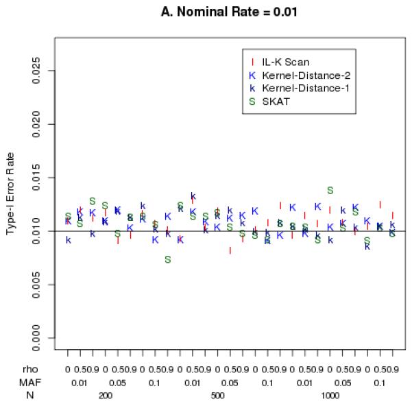
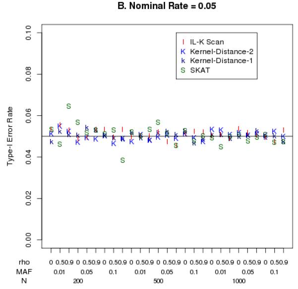
Empirical Type-I error rates at nominal levels 0.01 (panel A) and 0.05 (panel B).
Results for power when there is a single cluster are illustrated in Figure 3 for N=500 and in Figure 4 for N=1,000. For these simulations, the density of the cluster ranged from no clustering (density = 0.05, so 10 risk variants were randomly scattered among 200 variants), to the tightest clustering (density = 1, so all 10 risk variants were adjacent). The three statistics designed to detect clusters (IL-K scan and Kernel-Distance-1 and Kernel-Distance-2) showed increasing power as the cluster density increased, in contrast to the omnibus SKAT statistic whose power tended to remain constant over the different density values. Figures 3 and 4 also illustrate the influence of SNP correlations on power: increasing correlation tended to increase the power of both IL-K scan and Kernel-Distance statistics, yet increasing correlation tended to decrease power of SKAT. Surprisingly, when there was no clustering of variants (density = 0.05), the IL-K scan statistic had greater power than the SKAT statistic when the correlation among markers was large (ρ = .5,.9). This suggests that the IL-K scan statistic might be preferred over SKAT, even as an omnibus test for association, particularly in regions with large amounts of linkage disequilibrium. The Kernel-Distance statistics also tended to have greater power than SKAT when there was clustering of variants, or when the SNP correlation was large. The one-sided Kernel-Distance-1 tended to have greater power than the two-sided Kernel-Distance-2 when there was weak clustering (e.g., density = 0.1), but the two-sided version had greater power for stronger clustering. Furthermore, for strong clustering, the IL-K scan statistic tended to have greater power than the Kernel-Distance statistics.
Figure 3.
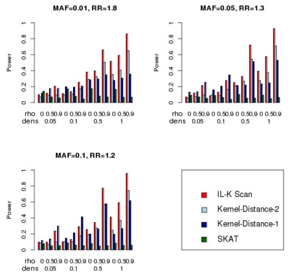
Simulated power for detecting one cluster (nominal Type-I error = 0.05), N = 500.
Figure 4.
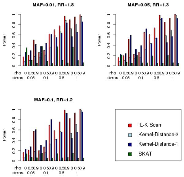
Simulated power for detecting one cluster (nominal Type-I error = 0.05), N = 1,000.
The patterns of relative power that we observed for one-cluster were repeated when we simulated two clusters, illustrated in Figure 5. These simulations were more limited than the range of parameters used for one cluster. For two clusters, we used N=1,000 subjects with greater cluster density (density of 0.5 and 1.0), each cluster containing 5 risk variants. This is because less dense clustering, of two clusters centered at 1/3 and 2/3 the length of the haplotype, would tend to resemble a single cluster spread over most of the haplotype. Figure 5 illustrates that the IL-K scan statistic had the greatest power, and the SNP correlations increased power for IL-K scan and Kernel-Distance statistics, yet decreased power for the SKAT statistic.
Figure 5.
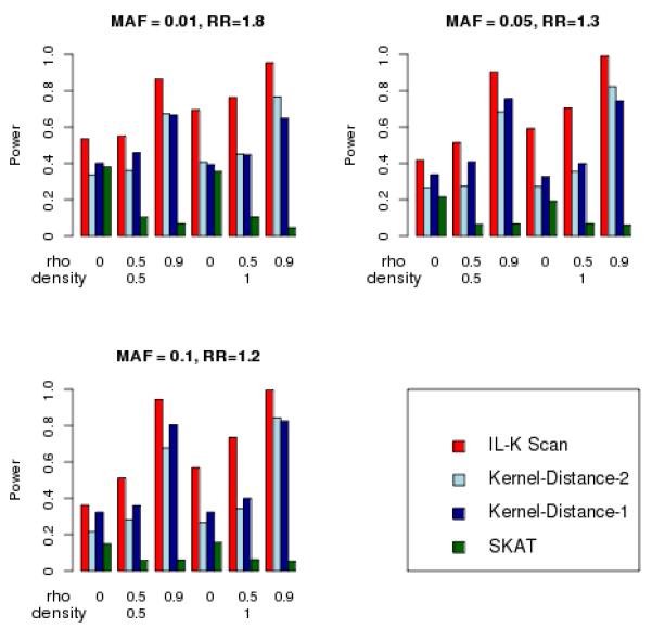
Simulated power for detecting two clusters (nominal Type-I error = 0.05), N = 1,000.
The computation time for the different simulation scenarios depended primarily on the sample size. For N=500, the range in computation time for SKAT was 8-12 sec (computation time for a simulation scenario was the trimmed mean over 1,000 simulations, trimming off the top 2%). For N=1,000, this range was 13-20 sec. The Kernel-Distance statistic took 3 to 8 times longer than SKAT, and the IL-K statistic took 7-14 times longer than SKAT.
Discussion
Statistical tests of clustering of genetic variants in a genomic region have potential to improve genetic association analyses by affording greater power, in contrast to omnibus tests of differences in variant frequencies between cases and controls. We extended Tango’s Kernel Distance statistic, originally developed for two-dimensional spatial clustering, to one-dimensional linear genomic clustering. By simulations, we found that the Kernel Distance statistics (one- and two-sided) and the IL-K scan statistic had greater power to detect genetic associations, when causal variants clustered, than the omnibus SKAT statistic. Furthermore, the IL-K scan statistic tended to have the greatest among the methods we evaluated. Although the IL-K scan statistic required more computation time than the Kernel Distance statistics, approximately twice the time, the computation times were reasonable for the number of genetic variants we evaluated (200) and the number of subjects (1000). This suggests that the preferred method would be the IL-K statistic.
Surprisingly, our simulations showed that even without clustering of variants, the IL-K scan statistic and Kernel Distance statistics could have greater power than the omnibus SKAT statistic to detect associations, mainly when the variants were correlated. Without correlation, SKAT tended to have the greatest power, but as correlation increased, the power of SKAT dramatically decreased. In contrast, both IL-K and Kernel Distance had increased power as correlation increased.
Acknowledgements
This research was supported by the U.S. Public Health Service, National Institutes of Health (NIH), contract grant number GM065450 (DJS, JPS).
References
- Asimit J, Zeggini E. Rare variant association analysis methods for complex traits. Annu Rev Genet. 2010;44:293–308. doi: 10.1146/annurev-genet-102209-163421. [DOI] [PubMed] [Google Scholar]
- Bansal V, Libiger O, Torkamani A, Schork NJ. Statistical analysis strategies for association studies involving rare variants. Nat Rev Genet. 2010;11(11):773–85. doi: 10.1038/nrg2867. [DOI] [PMC free article] [PubMed] [Google Scholar]
- Basu S, Pan W. Comparison of statistical tests for disease association with rare variants. Genetic Epidem. 2010;35:606–619. doi: 10.1002/gepi.20609. [DOI] [PMC free article] [PubMed] [Google Scholar]
- Breslow NE, Day NE. The analysis of case-control studies. Inter Agency Res Cancer; Lyon: 1980. [PubMed] [Google Scholar]
- Fier H, Won S, Prokopenko D, Alchawa T, Ludwig KU, Fimmers R, Silverman EK, Pagano M, Mangold E, Lange C. ‘Location, Location, Location’: a spatial approach for rare variant analysis and an application to a study on non-syndromic cleft lip with or without cleft palate. Bioinformatics. 2012;28(23):3027–33. doi: 10.1093/bioinformatics/bts568. [DOI] [PMC free article] [PubMed] [Google Scholar]
- Ionita-Laza I, Makarov V, Buxbaum JD. Scan-statistic approach identifies clusters of rare disease variants in LRP2, a gene linked and associated with autism spectrum disorders, in three datasets. Amer J Human Genet. 2012;90(6):1002–13. doi: 10.1016/j.ajhg.2012.04.010. [DOI] [PMC free article] [PubMed] [Google Scholar]
- Kulldorff M. A spatial scan statistic. Commun Stat Theory Methods. 2007;26:1481–1496. [Google Scholar]
- Kwee LC, Liu D, Lin X, Ghosh D, Epstein MP. A powerful and flexible multilocus association test for quantitative traits. Am J Hum Genet. 2008;82(2):386–97. doi: 10.1016/j.ajhg.2007.10.010. [DOI] [PMC free article] [PubMed] [Google Scholar]
- Lee S, Emond MJ, Bamshad MJ, Barnes KC, Rieder MJ, Nickerson DA, Christiani DC, Wurfel MM, Lin X. Optimal unified approach for rare-variant association testing with application to small-sample case-control whole-exome sequencing studies. American journal of human genetics. 2012a;91(2):224–37. doi: 10.1016/j.ajhg.2012.06.007. [DOI] [PMC free article] [PubMed] [Google Scholar]
- Lee S, Wu MC, Lin X. Optimal tests for rare variant effects in sequencing association studies. Biostatistics. 2012b;13(4):762–75. doi: 10.1093/biostatistics/kxs014. [DOI] [PMC free article] [PubMed] [Google Scholar]
- Mantel N. The detection of disease clustering and a generalized regression approach. Cancer Res. 1967;27:209–220. [PubMed] [Google Scholar]
- Ruppert D, Wand P, Carroll R. Cambridge University Press; Cambridge: 2005. Semiparametric regression. [Google Scholar]
- Tango T. The detection of clustering of disease in time. Biomertics. 1984;40:15–26. [PubMed] [Google Scholar]
- Tango T. A test for spatial disease clustering adjusted for multiple testing. Stat Med. 2000;19(2):191–204. doi: 10.1002/(sici)1097-0258(20000130)19:2<191::aid-sim281>3.0.co;2-q. [DOI] [PubMed] [Google Scholar]
- Tango T. Statistical Methods for Disease Clustering. Springer; New York: 2010. [Google Scholar]
- Wu MC, Lee S, Cai T, Li Y, Boehnke M, Lin X. Rare-variant association testing for sequencing data with the sequence kernel association test. Am J Hum Genet. 2011;89(1):82–93. doi: 10.1016/j.ajhg.2011.05.029. [DOI] [PMC free article] [PubMed] [Google Scholar]


