Quantitative cw Overhauser Dynamic Nuclear Polarization for the Analysis of Local Water Dynamics

Abstract

Liquid state Overhauser Effect Dynamic Nuclear Polarization (ODNP) has experienced a recent resurgence of interest. The ODNP technique described here relies on the double resonance of electron spin resonance (ESR) at the most common, i.e. X-band (~ 10 GHz), frequency and ¹H nuclear magnetic resonance (NMR) at ~ 15 MHz. It requires only a standard continuous wave (cw) ESR spectrometer with an NMR probe inserted or built into an X-band cavity. Our focus lies on reviewing a new and powerful manifestation of ODNP as a high frequency NMR relaxometry tool that probes dipolar cross relaxation between the electron spins and the ¹H nuclear spins at X-band frequencies. This technique selectively measures the translational mobility of water within a volume extending 0.5–1.5 nm outward from a nitroxide radical spin probe that is attached to a targeted site of a macromolecule. This method has been applied to study the dynamics of water that hydrates or permeates the surface or interior of proteins, polymers, and lipid membrane vesicles.

We begin by reviewing the recent advances that have helped develop ODNP into a tool for mapping the dynamic landscape of hydration water with sub-nanometer locality. In order to bind this work coherently together, and to place it in the context of the extensive body of research in the field of NMR relaxometry, we then rephrase the analytical model and extend the description of the ODNP-derived NMR signal enhancements. This extended model highlights several aspects of ODNP data analysis, including the importance of considering all possible effects of microwave sample heating, the need to consider the error associated with various relaxation rates, and the unique ability of ODNP to probe the electron–¹H cross-relaxation process, which is uniquely sensitive to fast (tens of ps) dynamical processes. By implementing the relevant corrections in a stepwise fashion, this paper draws a consensus result from previous ODNP procedures, and then shows how such data can be further corrected to yield clear and reproducible saturation of the NMR hyperpolarization process. Finally, drawing on these results, we broadly survey the previous ODNP dynamics literature. We find that the vast number of published, empirical hydration dynamics data can be reproducibly classified into regimes of surface, interfacial, vs buried water dynamics.

1. Introduction

To achieve ODNP enhancement, one adds molecules or moieties containing unpaired electron spins (i.e. spin probes) to the solution of interest and then irradiates with microwaves that significantly saturate the ESR transitions. Researchers have employed ODNP in this fashion for several decades in order to hyperpolarize nuclear spins in aqueous solutions at ambient temperatures and generate an NMR signal up to two orders of magnitude larger than the corresponding thermally polarized (i.e. typical) signal [1– 6]. However, researchers have only recently implemented ODNP towards the goal of quantifying hydration dynamics [7–9].

This new manifestation of ODNP takes advantage of the variable NMR signal enhancements observed when a spin probe is positioned in different molecular environments. As ODNP polarization transfer occurs by way of the time-dependent dipolar interaction between the unpaired electron spin of the spin probe and the nuclear spin of the water protons, it is selectively sensitive to water dynamics within 0.5–1.5 nm of the spin probe (i.e., 0.5–14 nm³). Because of this selective sensitivity, one can analyze the NMR signal enhancements to extract an unprecedented measurement of the local translational diffusivity (D_local) of the water [8, 10, 11]. With the proper analysis, even meager signal amplification can yield meaningful quantification of the local hydration dynamics [8–10, 12]. Well-established chemistry can attach stable nitroxide radical spin probes to targeted sites on proteins, lipid vesicles, synthetic polymers, and nucleic acids [13, 14]. Therefore, a series of differently placed spin probes allow one to map out the dynamics of the hydration water across an entire structural subunit [15, 16].

Here, we present an overview of recent developments that are relevant to the state of the art in detecting ODNP-derived local hydration dynamics. Given that the ODNP-derived quantification of local hydration dynamics around biomolecular systems is a new and emerging field, this review article will summarize both relevant existing studies as well as unpublished developments by the authors. We start with a focused review of the literature relevant to ODNP dynamics studies (Section 2), then present our viewpoint on which are the most important challenges associated with achieving quantitative ODNP analysis and how they can be overcome (Section 3), and finally report new findings that are critical for pushing ODNP hydration dynamics studies forward (Sections 4 and 5). In the latter sections, we focus on a set of developments and corrections that improve the accuracy of quantitative ODNP analysis and that permit its application to dilute samples with spin probe concentrations more than two orders of magnitude lower than previously feasible.

In particular, we present an intimate link between microwave-induced dielectric heating and NMR relaxation processes (Sections 4.1– 4.3) and provide a simple formalism that presents ODNP as a type of NMR relaxometry. This formalism can more consistently and accurately extract the coupling factor (ξ), which is the key ODNP parameter that has been used to quantify the hydration dynamics (Section 4.4), and it forms the basis for the previously unpublished results presented here. These focus first on the measurement of small spin probe molecules freely dissolved in bulk water. This “bulk coupling factor” measurement is of particular interest since it represents an important reference point for the study of hydration dynamics. The results presented here initially come to a consensus with recent results by the group of Bennati et al., who reported a bulk coupling factor of 0.32–0.33 (Section 5.3.2). However, we also find that even minimal dielectric heating affects the measurement of ODNP coupling factors by altering the NMR T₁ relaxation rates (Section 5.4.1); complete elimination of this effect yields a superior match between the ODNP data and model (Section 5.4.2), as well as a quantitatively different bulk coupling factor of 0.27 (Section 5.4.3). The success of these free spin probe studies also motivates us to reevaluate the prospect of improving ODNP as an analytical tool to study the hydration dynamics in and around complex molecular systems at the dilute concentrations crucial to biochemical studies – i.e. 100 μM and lower (Section 5.4.4). We conclude with a focused review of the ODNP hydration dynamics data in the literature and how these may be affected by the new method of analysis presented here (Section 5.4.5).

2. Review

The understanding of the physical processes underlying ODNP enhancement has remained relatively unchanged since Hausser and Stehlik presented their review [1], which shows how the steady-state solution of the Solomon equations [18] can predict ODNP enhancements. Subsequent research has applied this theory in a relatively unmodified form [3, 8]. The resulting model accurately predicts the ODNP enhancements for water that contains high (≥ 10 mM) concentrations of spin probes, whether freely dissolved in solution [3, 8, 17] or covalently tethered to slowly tumbling macromolecular systems [8, 9]. It is this model which introduced the coupling factor (ξ) – a parameter that determines the local efficiency of the ODNP polarization transfer and depends only on the motion of the water molecules relative to the spin probe.

For the sake of uniformity, we briefly clarify the notation we use throughout this paper. While some previous work by Han et al. [7–9, 12, 17, 20] has denoted the coupling factor by ρ, we use ξ, since (consistently with other literature [1, 1, 3, 21, 22]) we reserve ρ for the local self-relaxation rate (Table 1). Additionally, always using the term “relaxivity” to denote a concentration-scaled relaxation rate with units s⁻¹M⁻¹ (Table 2), we define a local self-relaxivity, k_ρ, related to the self-relaxation rate as follows

Table 1.

Comparison between notation previously used by Han et al. (e.g. [8, 17]), and notation used here.

	Previous Notation of Han et al.		Present Notation
self-relaxation rate	kC	⇒	kρC
coupling factor	ρ	⇒	ξ

Table 2.

Each column summarizes an equivalent means for denoting a quantity. Wherever possible, all notation matches that of Solomon [18] and Hausser [1]. Since this work explores various concentration-dependent effects, it principally makes use of the concentration-independent relaxivities, k_ρ and k_σ (even though this notation is not used elsewhere). Since k_ρ and k_σ quantify relaxation processes localized (i.e. ∝ r⁻⁶) around the spin probe, they provide interesting information about the local hydration dynamics, complementary to information derived from the coupling factor, ξ (compare, for instance to [10, 19]). This article does not make use of the transition rate notation [1, 18], but it is provided here in the third column for comparison. The relaxivities (k_σ and k_ρ) have units [ s⁻¹M⁻¹], and T_1,0 has units [s].

	Standard Symbol	Quantity as a function of:
		Relaxivities	Transition Rates
local dipolar self-relaxation rate	ρ	kρC	w0 + 2w1 + w2
local dipolar cross-relaxation rate	σ	kσC	w2 − w0
coupling factor	ξ	$\frac{k_{\sigma }}{k_{\rho }}$	$\frac{w_2-w_0}{w_0+2w_1+w_2}$
leakage factor	f	$\frac{k_{\rho }C}{k_{\rho }C+T_{1,0}^{-1}}$	$\frac{w_0+2w_1+w_2}{w_0+2w_1+w_2+w^0}$
nuclear longitudinal relaxation rate	$T_1^{-1}$	$k_{\rho }C+T_{1,0}^{-1}$	w0 + 2w1 + w2 + w0

$$\rho =k_{\rho }C.$$ (1)

This expression makes the dependence of ρ on the spin probe concentration, C, apparent. Similarly, we define a local cross-relaxivity parameter, k_σ, that allows us to express the concentration dependence of the cross-relaxation rate, σ,

$$\sigma =k_{\sigma }C.$$ (2)

Both k_σ and k_ρ arise from time-dependent dipolar interactions that scale with the distance (r) between the spin probe electron and the water proton as r⁻³. These time-dependent interactions give rise to transition rates, and therefore relaxivities, that scale as r⁻⁶ [18]. Thus, both k_σ and k_ρ depend only on the dynamics and amount of water that very closely (0.5–1.5 nm) approaches the spin probe. The balance between k_σ and k_ρ determines the unitless coupling factor, ξ, as detailed by Hausser [1], i.e.

$$\xi =\frac{\sigma }{\rho }=\frac{k_{\sigma }}{k_{\rho }}.$$ (3)

Following previous literature, we uniformly denote the sample’s proton longitudinal relaxation time as T₁ for samples that contain spin probes and as T_1,0 for the same samples, but with the spin probes excluded. The T_1,0 is not only relevant to characterize samples without spin probes, but also to quantify the background NMR (proton) relaxation rate ( $T_{1,0}^{-1}$) of the water molecules in the absence of dipolar coupling to the spin label. For instance, at biologically relevant concentrations of 100 μM and lower, water molecules spend most of their time passing through the bulk solvent more than 1.5 nm from the spin probe, where their relaxation is determined exclusively by T_1,0.

2.1. Review of Previous Theory

The polarization transferred from the electron spin to the protons is inverted relative to the thermal polarization of the protons. Thus, suffficient amounts of polarization transfer lead to an enhanced and inverted NMR signal. As shown by Hausser and Stehlik [1], the nuclear population, 〈I_z〉, relaxes at a rate set by the background ( $T_{1,0}^{-1}$), self- (k_σC), and cross-relaxation (k_ρC) processes

$$\frac{d\langle I_z(t)\rangle }{dt}=-(k_{\rho }C+T_{1,0}^{-1})(\langle I_z(t)\rangle -I_0)-k_{\sigma }C(\langle S_z\rangle -S_0),$$ (4)

where 〈S_z〉 gives the electron spin population, which is continuously saturated by resonant microwaves, and S₀ and I₀ give the equilibrium polarizations. The enhancement, E, is defined as the ratio between the ODNP-enhanced proton signal and the thermal signal, E = 〈I_z〉/I₀. The electron spin saturation factor, s(p), is defined as

$$s(p)=\frac{S_0-\langle S_z(p)\rangle }{S_0},$$ (5)

where p is the power of the saturating microwave irradiation. Substituting these definitions into Eq. (4) and noting that S₀/I₀ ≈ ω_e/ω_H yields

$$\frac{dE(t)}{dt}=\left(k_{\rho }C+T_{1,0}^{-1}\right)(1-E)-k_{\sigma }Cs(p)\left|\frac{{\omega }_e}{{\omega }_H}\right|$$ (6)

where, for a nitroxide in aqueous solution |ω_e/ω_H| = 659.33 ± 0.05 [23]. We will find it convenient to refer to 1 − E (which is referred to in other literature as “ε” or “−ε”, e.g. [24]) as the “amount of polarization transferred” [25]. Following Hausser one can solve Eq. (6) for the steady-state solution (i.e. dE/dt = 0) of 1−E(p). Using the definitions of ξ, and f given in Table 2 (and explained further below), this yields

$$1-E(p)=\xi s(p)f\left|\frac{{\omega }_e}{{\omega }_H}\right|,$$ (7)

where the unitless coupling factor, ξ, leakage factor, f, and saturation factor, s, all affect the efficiency with which electron spin polarization transfers to the nuclear spin polarization. Our focus here is to accurately isolate the coupling factor, ξ, which depends exclusively on the local dipolar transition rates and, therefore, exclusively on information related to the local hydration dynamics.

The leakage factor, f, gives the proportion of the total proton relaxation that is due to the local dipolar relaxation mechanisms [26], i.e.

$$f=\frac{k_{\rho }C}{k_{\rho }C+T_{1,0}^{-1}}.$$ (8)

Since the total NMR relaxation rate of a solution containing a spin probe ( $T_1^{-1}$) is the sum of the bulk ( $T_{1,0}^{-1}$) and the local dipolar (k_ρC) relaxation rates, i.e.

$$T_1^{-1}=k_{\rho }C+T_{1,0}^{-1},$$ (9)

the leakage factor can also be written as

$$f=1-\frac{T_1}{T_{1,0}}.$$ (10)

and can be obtained from inversion recovery experiments that determine T₁ and T_1,0 from samples, respectively, with and without added spin probe.

Finally, we turn to the saturation factor, s(p). In the absence of microwave power, s(p = 0) = 0. With increasing microwave power (p), s(p) asymptotically approaches a maximal value of s_max. As explained below, a variety of factors contribute to determining the value of s_max, which ranges $\frac{1}{3}\le s_{\mathit{max}}\le 1$ for ¹⁴N nitroxides. Fortunately, for most biological samples with tethered spin probes, a choice of s_max ≈ 1 is a good approximation (Section 2.2). The transition between s(p = 0) = 0 and s(p → 1) = s_max is given for well separated Lorentzian absorption lines by standard ESR theory [17, 27, 28]:

$$s(p)=\frac{p{s}_{\mathit{max}}}{p_{1/2}+p}.$$ (11)

Substituting this into Eq. (7),

$$1-E(p)=\xi f\left|\frac{{\omega }_e}{{\omega }_H}\right|\frac{p{s}_{\mathit{max}}}{p_{1/2}+p}.$$ (12)

Here, p_1/2 is the power needed to achieve half of the maximum possible saturation. A variety of factors, including the electron spin relaxation time and the electrical properties of the resonant cavity combine to determine the value of p_1/2. One can eliminate the dependence of E(p) on p_1/2 by extrapolating the enhancements to their asymptotic limit

$$\underset{p\to \infty }{lim}E(p)\equiv E_{\mathit{max}},$$ (13)

to give (via Eqs. (7) and (11))

$$1-E_{\mathit{max}}=\xi s_{\mathit{max}}f\left|\frac{{\omega }_e}{{\omega }_H}\right|.$$ (14)

Later (in Section 4.4), we will clarify how, as a result of dielectric heating, Eq. (14) is in practice an approximation – especially at lower spin probe concentrations. Specifically, Eq. (14) relies on the assumption that f remains constant with respect to microwave power, which turns out to be inaccurate in the presence of even small dielectric heating. Therefore, we will refer to it as the “uncorrected model.”

In summary, the previous (i.e. uncorrected) model advises one to determine the ODNP signal enhancement at several values of microwave power and to fit the resulting signal enhancements to Eq. (12), so that they can be extrapolated to an asymptotic high-power limit, E_max. The value of E_max is then inserted into Eq. (14), along with the value of f (Eq. (10)) and the value of s_max, which can be determined through one of several means discussed in the next section (Section 2.2). This yields the value of ξ, which (as will be discussed in Section 2.5) one can analyze with an appropriate dynamic model to quantify the motion of the permeating or hydrating water molecules located near the spin label.

2.2. Maximal Saturation Factor

Typical nitroxide-based spin probes have two (in the case of ¹⁵N nitroxide) or three (in the case of ¹⁴N nitroxide) hyperfine transitions, arising from coupling between the nitrogen nucleus and the electron spin. Since these are separated by ~60 MHz, only one hyperfine transition at a time can typically resonate with the saturating cw microwaves. This leads to a situation where the ODNP saturation factor, s(p), is distinct from the saturation factor that can be determined by standard cw ESR experiments. While standard cw ESR power saturation experiments can read out the saturation of the resonant transition, ODNP depends on the net saturation of all three (or two) ESR transitions. Both Heisenberg exchange between colliding nitroxide molecules and the longitudinal relaxation of the nitroxide’s nitrogen nuclear spin can mix the saturation between the resonant and non-resonant populations. Thus, the value of s_max will vary depending on the rate of this mixing.

Initially, Bates and Drozdoski developed a model of the ODNP saturation factor that included a Heisenberg exchange rate dependent contribution from the non-resonant transitions [28]. Armstrong and Han [17] extended this analysis by adding the effects of nitrogen nuclear spin relaxation, which exceeds the Heisenberg exchange rate for many chemically tethered spin probes, especially those tethered to large molecular systems, such as proteins or lipid membrane assemblies. The resulting analysis was, at the time, the most complete analysis of the key mechanisms behind the ODNP saturation factor. It yields s_max as a function of the Heisenberg exchange rate, which varies with spin probe concentration, and the nitrogen nuclear spin relaxation rate, which does not vary with spin probe concentration. By determining the value of ξs_max (cf. Eq. (14)) for freely dissolved spin probes over a series of concentrations and fitting the results to their model for s_max, they were able to eliminated the dependence on s_max, yielding a value of ξ_bulk = 0.22 for freely dissolved spin probes. Notably, drawing on ELDOR measurements by Robinson et al. that report on very fast nitrogen relaxation times for more slowly tumbling molecules [29], they also predicted that the s_max for spin probes tethered to biological or polymer samples (which are typically large and therefore slowly tumbling) should closely approach 1 [17].

Türke and Bennati have since used pulsed ESR on ¹⁵N nitroxides to directly interrogate the non-resonant contribution to s_max [3, 30]. They also turned the attention of the ODNP community toward the earlier work of Hyde, Chien, and Freed, who employed a double resonance cavity to partially saturate one hyperfine transition while observing the reduction, R, in a different hyperfine transition. The value of R quantifies the partial saturation of the non-resonant hyperfine transitions [31]. We can deduce that the value of R is directly related to s_max; for ¹⁴N nitroxides,

$$s_{\mathit{max}}=\frac{1}{3}-\frac{2}{3}R$$ (15)

and for ¹⁵N nitroxides

$$s_{\mathit{max}}=\frac{1}{2}-\frac{1}{2}R.$$ (16)

These equations allow us to substitute the appropriate expression for R from Ref. [31] in order to determine s_max for any situation. For instance, freely dissolved spin probes exhibit significant Heisenberg exchange but negligible nitrogen relaxation, so that (for ¹⁴N)

$$s_{\mathit{max}}=1-\frac{2}{3+3b^{″}},$$ (17)

where, following Ref. [31], b″ = w_h/6w_e gives a ratio between the rate of Heisenberg exchange, w_h, and the rate of electron longitudinal relaxation, w_e. (In the case where both Heisenberg exchange and nitrogen relaxation are active, more complex expressions for R are also available from Ref. [31].) Notably, however, the Heisenberg exchange of free nitroxide probes in water was not quantified in Ref. [31]. Türke and Bennati [30] employed modern pulsed ELDOR measurements to quantify both w_h and w_e for ¹⁵N nitroxides and found a value of b″ = C × 198.7 M⁻¹, where C is the spin probe concentration. They also placed this measurement in context by using it to determine the value of s_max in Eq. (14) and thus extract the ODNP coupling factor, which they reported to be 0.33.

Interestingly, the Hyde and coworkers also advanced the earlier methodology of Ref. [31] and applied it to biologically relevant systems; most notably, they performed measurements on doxyl-stearic acid spin probes in lipid bilayers at 27°C. Despite the fact that their spin probe is more mobile than many spin probes attached to proteins or at other locations in the lipid bilayer (and should exhibit a correspondingly slower nitrogen relaxation), they retrieved a value of the nitrogen relaxation that corresponds to s_max = 0.92 [32]. This confirms Armstrong and Han’s hypothesis in Ref. [17] that s_max approaches 1 for tethered nitroxide probes, even when Heisenberg spin exchange rates are low. However, as the overall accuracy of quantitative ODNP improves, a more accurate determination of s_max with at least two significant figures will become increasingly relevant.

Together, these three methods (the spin probe concentration series, pulsed ELDOR, and the approximation that s_max ≈ 1 for most tethered spin probes) provide a fairly complete toolbox that allows one to determine s_max and extract an accurate value of ξ under a variety of circumstances.

2.3. Two Variants of ODNP

Among other reasons, the different methods for calculating the saturation factor have caused a separation of ODNP into two different methods or strategies. Each variant has – until now – also generated different quantitative results: One variant (cw ODNP) retrieves the necessary information from the NMR signal while relying solely on the use of a cw microwave source that saturates the ESR transition (as in Refs. [8, 17, 33]), while the other (ELDOR-assisted ODNP) relies at least partially on the ability to apply microwave pulses and detect the resulting ESR free induction decay or spin echo (as in Refs. [3]). ELDOR-assisted ODNP has shown promise by rectifying the value for the bulk coupling factor (i.e. for bulk water near a small, freely dissolved nitroxide probe molecule), yielding results that agree more closely with the predictions of field cycling relaxometry (FCR) [8, 30] and molecular dynamics (MD) [34] studies. Meanwhile, various recent studies have shown that the more widely accessible cw ODNP variant shows promise as a routine approach for the determination of local hydration dynamics [8, 10–12]. Thus far, only the cw ODNP method has been applied to the quantification of hydration water dynamics in biological and soft matter systems. However, a controversy over the accuracy of cw ODNP has persisted because it was believed to report a value of the bulk coupling factor [8] that strongly disagreed with the value predicted from FCR results or the value observed by ELDOR-assisted ODNP.

2.4. ODNP for High Field and Medical Applications

The search for a hyperpolarization method applicable to solution samples under ambient conditions has driven a variety of other recent ODNP studies that are focused not on retrieving hydration dynamics, but on harvesting optimal polarization from ODNP experiments for use in high-resolution NMR spectroscopy. Notably, these include: an NMR spectrometer that achieves field cycling through shuttling and can perform ODNP with microwave excitation at up to 1.4 GHz, novel ODNP probe designs optimized for high-field ODNP (a more recent design is also presented in [35]), studies of coherently coupled dynamics achieved in the low field limit, pulsed-microwave experiments with ESR resonance frequencies at 1.4 GHz and 300 MHz, and most importantly, the unexpectedly high ODNP enhancements achieved at ESR resonance frequencies of 260 GHz and higher. Griesinger et al. have summarized these and other developments in a recent review [36]. Therefore, even though the body of work reviewed therein is very relevant to the future deployment of ODNP dynamics studies at high field, we do not include a detailed reevaluation here.

It is necessary to mention two important advances pertaining to the ODNP enhancement of aqueous solutions that have not yet been applied to the study of hydration dynamics, but were also not reviewed in Ref. [36]. The novel non-radiative microwave resonator design presented by Annino et al. [37, 38] provides very high ESR performance at 95 GHz, easily integrates DNP functionality, and can be fabricated from commonly available materials. Researchers have also employed ODNP hyperpolarization to enhance perfusion imaging, where the first proof of principle application by Han et al. [39] was followed by further development and applications at 10 GHz (ESR) [40–43], an extension to higher frequencies (35 GHz ESR) by Krummenacher et al. [44], and a recent in vivo study demonstrating enhanced visualization of brain perfusion in a live rat [45].

2.5. Interpretation of ξ

Again returning to our focus on the study of hydration dynamics, we discuss how one can translate the ODNP coupling factor, ξ, into a more intuitive measure of water dynamics. Both a simplified model of translational diffusion [46] and the more sophisticated force-free hard-sphere model [47] (FFHS, discussed next) can analytically translate the value of the coupling factor, ξ, into a translational correlation time, τ_c. We will conclude by reviewing the FFHS model for the coupling factor, but first discuss how the resulting τ_c value is related to hydration dynamics.

Physically, this correlation time can be described as the lifetime of the dipolar interaction between the electron spin of the spin probe and the proton spin of the water molecule, and it is related to the diffusivity between the two:

$${\tau }_c=\frac{d^2}{D_{\mathit{local}}+D_{SL}}$$ (18)

where D_local is the diffusivity of the hydration water within 0.5–1.5 nm of the spin probe, D_SL is the diffusivity of the spin probe, and d is the “distance of approach” between the water and the spin probe [48].

Armstrong and Han [8] pointed out that if we assume that the distance of approach, d, will fit to a similar value in different local environments, we can compare the correlation time, τ_c,site, for a site with a tethered spin probe to that of a spin probe freely dispersed in bulk water, τ_c,bulk, in order to quantify the local diffusivity of the water near the spin probe. Since for τ_c,site on macromolecules, D_SL ≪ D_local, we see that

$$D_{\mathit{local}}\approx \left(\frac{{\tau }_{c,\mathit{bulk}}}{{\tau }_{c,\mathit{site}}}\right)(D_{H_{2}O}+D_{SL,\mathit{free}}).$$ (19)

where D_H2O = 2.3 × 10⁻⁹ m²s⁻¹, is the bulk water diffusion (around the freely dissolved TEMPO spin probe) and D_SL,free = 4.1 × 10⁻¹⁰ m²s⁻¹ is the diffusivity of the small TEMPO spin probe [8]. Therefore, more compactly,

$$D_{\mathit{local}}\approx \left(\frac{{\tau }_{c,\mathit{bulk}}}{{\tau }_{c,\mathit{site}}}\right)2.7\times {10}^{-9}{\text{m}}^2{\text{s}}^{-1}.$$ (20)

It is important to note that the translational correlation time is not necessarily a uniquely defined property of the molecular dynamics of a particular system. Rather, its exact value will also depend on the nature of the interaction probed by a particular measurement [49]. Thus, we can expect that, even though they should exhibit similar trends and relative values, the translational correlation times obtained by dynamics Stokes shift spectroscopy [50], dipolar relaxation driven ODNP [8], as well as various scattering measurements [51–53] might yield different absolute numbers, even though the relative trends should remain. By analogy, the rotational correlation time differs for different measurements, depending on whether the measurement probes the relaxation of an interaction that depends on rank one spherical harmonics (e.g. dielectric spectroscopy) or rank two spherical harmonics (e.g. NMR quadrupolar relaxation) [54–57]. This highlights the usefulness of converting the translational correlation time (even approximately) into a local translational diffusion coefficient, D_local, which is uniquely defined based solely on the local molecular dynamics.

The specific fashion in which changes to the overall timescale of the dynamics (i.e. τ_c) affect the measured value of ξ is described and quantified by the spectral density function for the dipolar interaction between the spin label and the water. By choosing an analytical expression for this spectral density function, one can easily convert the measured value of ξ into a correlation time, τ_c. As in previous literature (e.g. [3, 8, 10, 17, 19, 58]) we employ Hwang and Freed’s [47] expression, which is based on a force free hard sphere (FFHS) model of translational diffusion. The reduced FFHS spectral density function is given by

$$J(\omega ;{\tau }_c)=\mathfrak{R}\mathfrak{e}\left[\frac{1+\frac{z}{4}}{1+z+\frac{4z^2}{9}+\frac{z^3}{9}}\right]$$ (21)

where

$$z\equiv \sqrt{i\omega {\tau }_c}.$$ (22)

The semicolon denotes that τ_c is a parameter; when we choose a particular value of τ_c, the FFHS model returns a spectral density function J(ω) that quantifies the average amplitude (or “density”) of the fluctuations in the spin-spin dipolar interactions for all angular frequencies ω. The coupling factor is determined by sampling the resulting spectral density function, J(ω), at particular combinations of the proton (ω_H) and the electron (ω_e) spin resonance frequencies, as follows:

$$\xi (B_0;{\tau }_c)=\frac{6J({\omega }_e-{\omega }_H;{\tau }_c)-J({\omega }_e+{\omega }_H;{\tau }_c)}{6J({\omega }_e-{\omega }_H;{\tau }_c)+3J({\omega }_H;{\tau }_c)+J({\omega }_e+{\omega }_H;{\tau }_c)},$$ (23)

yielding ξ as a function of τ_c and the static field, B₀, employed in the ODNP experiment. The dependence on B₀ arises because the two resonance frequencies are products of their respective gyromagnetic ratios (which are constants) with the magnetic field, i.e.

$$\begin{array}{l}{\omega }_e={\gamma }_e{B}_0=\frac{g{\mu }_B}{\hslash }{B}_0\\ {\omega }_H={\gamma }_H{B}_0.\end{array}$$

The form of Eq. (23) always applies when a dipolar interaction between the electron and nuclear spins can be assumed, regardless of the particular choice of the model used to determine the spectral density function, J(ω) [1]. Finally note that ω and τ_c are not independent variables in the reduced FFHS model given by Eq. (21), whose shape depends only on the product ωτ_c; the same is true for many other models. Thus, by moving to higher (lower) fields and frequencies one could probe faster (slower) motions more sensitively.

In the experiments presented and discussed here, we employ a static field (B₀ = ω_H/γ_H) corresponding to experimental NMR resonance frequencies near ω_H/2π = 15 MHz [59]. The coupling factor is thus determined by using the FFHS model to calculate $\xi \left(\frac{(2\pi )15\text{MHz}}{{\gamma }_H};{\tau }_c\right)$ as a function of the parameter τ_c (as presented in Fig. 1), then finding the value of τ_c that yields the experimentally determined ξ value. For instance, in Section 5, we will confirm a result of ξ_bulk = 0.33 when the uncorrected ODNP analysis is used, while a value of ξ_bulk = 0.27 is found after correction for the effect of temperature on the nuclear spin relaxation, or by careful elimination of any residual heating effects. These yield correlation times of τ_c,bulk = 33.3 ps and τ_c,bulk = 54 ps, respectively.

Figure 1.

ODNP, which measures the coupling factor, ξ, (solid blue line) exhibits a better selectivity for high-frequency (typically translational) motions of the solvent than an NMR relaxometry measurement that measures the self-relaxivity of the water in the presence of the spin probe, k_ρ, (dashed green line). The calculations shown here use the force-free hard sphere diffusion model at a field strength of 0.35 T (15 MHz NMR resonance); for both measurements, the range of correlation times probed will scale inversely with field [108].

At this point, it is important to note several obvious ways in which one could advance beyond the FFHS model. First, the original work by Hwang and Freed [47, 60] includes not just the FFHS model, but a general methodology for modeling the spectral densities of interactions between pairs of spins that could take into account, or (used deductively) potentially help describe, features of the radial distribution function between the spin probe and the water. Furthermore, Kruk et al. [61] and Kruk and Kowalewski [62, 63] have put forth a significant body of work, both to further these methods, and to advance the field of relaxation theory in general, in order to treat more difficult situations than the simple nitroxides used now, e.g. Gd³⁺ based relaxation agents. Once the experimental bottlenecks for ODNP discussed below have been overcome, such models may prove useful for developing a deeper understanding of the dynamics, e.g. analyzing exchange between different populations of water and more intimately probing the relationship between the local water structure and dynamics.

Ultimately, however, any model for the spectral density function that is parameterized by only one or two correlation times might prove limited, especially for complex biomolecular systems. Therefore, molecular dynamics (MD) simulations will likely play an important role in interpreting coupling factors with greater detail and rigor. At present, this task is non-trivial, since the most common water models are not able to quantitatively reproduce important dynamic parameters, such as the diffusion coefficient or the dielectric rotational correlation time of water [64–66]. Furthermore, trajectories several tens of ns long would be needed to fully model the relaxation processes relevant to ODNP.

Nonetheless, several researchers have already usefully applied MD to the study of ODNP. Armstrong, Soto, Shea, and Han [67] modeled the local diffusivity of water near small spin probes to confirm that the differences in structure between common spin probes did not have a significant effect on the hydration dynamics and that the local water dynamics near the freely dissolved spin probe is indistinguishable from that of bulk water. Sezer et al. [34, 68] were the first to calculate the coupling factor directly from molecular dynamics (MD) simulations; at X-band, they predicted a reasonable value of 0.30, and also accompanied their presentation with density matrix simulations of the spin physics. They explicitly calculated a spectral density function that was controlled by multiple distinct correlation times. In other words, they determined an alternative to Eq. (21) for their specific molecular system, where J(ω; τ_c,1, τ_c,2, …) was parameterized by multiple independent τ_c values, rather than just one. As a result of this observation, they were able to show show that the MD simulations are consistent with the observation of ODNP enhancement at higher fields, which exceeded the values predicted by analytical rotational or translational models of the dynamics. Very recently, Sezer [69] presented a method that overcomes the need for very long MD trajectories. This method seamlessly combines the best aspects of both analytical and MD models of relaxation: analytical methods handle the long timescales and distances, where they perform well, while the MD models describe the local dynamics near the spin probe, which are crucially linked to the complex local structure of the molecules under study, and which are overlooked by the approximations of analytical models, such as the FFHS model. The value of this method should prove especially relevant when the spin probe is tethered to macromolecular surfaces.

Very recently, Doll and Jeschke proposed using the value of the ODNP polarization transferred (1 − E) directly. They are able to retrieve reproducible measurements of the polarization transferred for samples with a spin probe concentration as low as 10 μM. They point out that in true protein systems, isotropic models of water dynamics, such as the FFHS model, may not be the appropriate tool for accurately analyzing the hydration dynamics. Thus, one can avoid both the benefits and the pitfalls alluded to earlier in this section by presenting a more qualitative parameter that describes water accessibility. Through application to select spin-labeled protein systems, they are able to empirically demonstrate that ODNP can measure the accessibility of the spin probe to the aqueous solvent in complex and important biomolecular systems, such as an ABC transporter protein embedded in lipid membranes [24].

2.6. Relaxometry

In the context of advancing our understanding of the dynamics near spin probes and the models that can be used to understand them, we should discuss a superficially different, but physically related, method – NMR field cycling relaxometry (FCR). Bennati et al. [58], Luchinat and Parigi [70], Höfer et al. [71] provided the first demonstration that FCR could help predict ODNP coupling factors. As noted earlier, Armstrong and Han [8] found that DNP and FCR measurements disagreed as to the value of the coupling factor (0.22 vs. 0.36, respectively). In a more detailed FCR study, Bennati et al. [58] then similarly predicted a coupling factor of 0.33–0.35, which compared well with their measurements that relied on the combination of ODNP and ELDOR to determine ξ. A very relevant and extensive body of work presents the use FCR to measure the hydration dynamics near spin probes [19, 72–74]; like the ODNP studies discussed here, this work reads out hydration dynamics through their affect on fluctuating dipolar spin interactions, and it places a particular emphasis on biologically relevant systems.

Physically, the main differences between FCR, or NMR relaxometry in general, and ODNP are related to the sensitivity and to the selectivity – i.e. how well the method selects for a particular timescales of motion. These differences are central to the reasons for beginning to pursue ODNP as a quantitative tool for investigating the hydration dynamics, in particular focusing on its viability for biological systems. As shown by Fig. 1, ODNP responds very selectively to fast timescale motion (i.e. ω_eτ_c < 1), which, at 0.35 Tesla (X-band), corresponds to τ_c values between 10 ps and 1 ns – i.e. the timescale for translational motion of bulk and loosely bound water [1]. The 659-fold difference in the Boltzmann polarization of the NMR and ESR resonance frequencies does not merely lead to a blanket enhancement of the NMR polarization. Rather, as the differential enhancement rate equation (Eq. (6)) points out, it selectively enhances the cross-relaxation rate by a factor of 659s(p). Thus, compared to conventional relaxometry methods, one can use 659 times smaller spin probe concentration in ODNP and still determine k_σ accurately – a point that we will return to in Sections 4.4, 5.3 and 5.4.4.

2.7. Hardware Design and Temperature Measurements

To help us address the practical details of performing analytical ODNP measurements, we find it useful to review a variety of resonator designs suitable for ODNP. Many of the experiments associated with the Han group employ a modular design, i.e. a separate microwave amplifier and source dedicated to ODNP and an NMR probe that inserts into an otherwise typical ESR cavity, as detailed in [33]. We will return to a more detailed analysis and improvement of such modular probe systems in Section 5.2. For now, we note that while the frequency of the ODNP source must be set separately, Lingwood, Han, Bhattacharya, et al. [7, 40, 45] have demonstrated how this means it can be transported and used in unusual situations, such as in the fringe field of a clinical MRI magnet. Also, because the ODNP accessory can be completely removed, difficult-to-acquire building materials, such as high-quality dielectric resonators or precision-machined cavities, can be seamlessly employed for high-sensitivity ESR (without an ODNP probe). The Bennati group adopted a different strategy, performing X-band DNP experiments with a commercial amplifier added on to the output of an ESR spectrometer, and re-purposing commercial ENDOR probes as DNP probes [3, 30]. Most recently Doll et al. [24] presented a high-quality home-built resonator, which includes a resonant NMR probe firmly mounted inside a dielectric resonator. Both the NMR and ESR performances of this device are excellent.

A detailed ability to analyze the sample heating occurring in different ODNP probes will undoubtedly allow discrimination between these designs and guide future design. At X-band frequencies (near 10 GHz and 3 cm wavelengths) and higher, the generation of a significant magnetic field (i.e. B_1,μw) inside a finite-sized sample necessarily implies the generation of an electric field (E_μw) that will heat aqueous samples, even if only to a small extent. The methods outlined here will help identify probes that optimize the B_1,μw/E_μw ratio. This is the key performance parameter for an ODNP resonator, since its maximization will yield maximum saturation, s(p), of the ESR resonance per unit of dielectric heating. These methods can also help identify which probes can best dissipate residual dielectric heating to the surrounding environment.

Bennati et al. [3] have directly observed the sample temperature of very large samples (≥ 0.9 mm i.d.) with an optical sensor and recorded temperature increases of up to 70°C. However, this sensor cannot be used with smaller diameter samples, which should exhibit less heating and therefore present more ideal ODNP samples. They estimate the heating in the smaller diameter samples based on the dielectric loss, which they calculate from changes in the microwave cavity Q factor. For instance, they predict an increase of sample temperature of at least 20°C for a sample with 0.45 mm diameter and 10 mm length. They also demonstrated a procedure for minimizing sample heating by carefully constraining the sample volume to the region of minimal electric field, resulting in negligible dielectric loss for a sample with 0.45 mm diameter and 3 mm length (i.e. 1.9 μL volume). However, many conventional cw ESR setups cannot measure changes in Q at high power with the precision required to measure these dielectric losses. This strategy may also overestimate the sample temperature, since it does not account for any heat transferred away from the sample and into the air that cools the cavity, which will become increasingly important with increased flow rates and decreased sample diameters. Furthermore, the temperature predicted based on dielectric losses did not agree well with the measurement of the temperature sensor for microwave irradiation times longer than 4 s. Routine hydration dynamics experiments on biological samples require easily repeatable and verifiable measurements of sample heating that can be carried out concurrently with cw ESR and ODNP measurements in the same instrumental setup.

A model of high field ODNP developed by Van Bentum et al. includes the effects of sample heating in order to predict the ODNP enhancements with the purpose of achieving maximal signal enhancements. They are able to model the enhancements for a series of aqueous solutions of free spin probes with concentrations of 10 mM and higher [75]. Like in other high-field ODNP studies (e.g. [76]), they measure the chemical shift of water to determine the sample temperature. However, for many ODNP studies of hydration dynamics, since the chemical shift of water presents a temperature variation of only 0.01 ppm/°C [77, 78], this technique is intractable, particularly at X-band fields (~ 0.35 T).

Sections 4.2 and 5.2 will demonstrate how the temperature variation of the bulk water, T_1,0, which researchers characterized and modeled over 35 years ago [56], provides a sensitive and practically useful intrinsic probe of sample temperature in an ODNP experiment. We will propose its application towards further advances in quantitative ODNP, through optimization of ODNP hardware and iterative correction of temperature effects. At the present time, it allows us to design and confirm small, but meaningful, improvements in the probe design. This strategy has not yet been compared to a strategy very recently presented by Doll et al. [24], which employs the thermal Boltzmann polarization of the NMR spins as a useful intrinsic probe of temperature, and presents some of the same benefits as the T_1,0 strategy for temperature tracking covered in Sections 4.2 and 5.2.

As a final side-note pertaining to future efforts to mitigate sample heating, it is relevant to note that Un et al. [79] implemented pulsed solid-state Overhauser-Effect DNP (in an organic conductor) at 140 GHz. This and similar techniques offer great promise for reducing the heat deposited by the saturating microwaves, but again would rely heavily on a facile means for temperature measurement.

It is important to emphasize that despite significant advances in probe design, temperature measurement, and saturation techniques, the dielectric heating still introduces measurable changes in the bulk water relaxation time. As described in Section 4, even small changes in bulk water relaxation time lead to measurable changes in the ODNP parameters, especially for samples with low concentrations (i.e. ≤ 500 μM) of nitroxide spin probes. Furthermore, anticipating the corrected model presented here, we point out that even in cases where careful hardware design does not completely remove all effects of heating, a proper assessment of the sample temperature can be incorporated into the model for the ODNP enhancements to retrieve more accurate results.

3. Perspective

As a bridge between the preceding review section and our newly presented theory, results, and final conclusions, we succinctly outline our personal perspective and strategies for advancing the ODNP hydration dynamics methodology:

Technical and experimental challenges have presented the principle bottleneck to advancing the ODNP methodology as a routine and reliable tool. As previously outlined, various exciting theoretical models have already been developed. Detailed comparison of the coupling factor (ξ) values that these models predict to experimental results could shed light on questions about the validity of various dynamic models, especially if measurements could be performed over a continuous range of fields and frequencies. However, to allow such a comparison, the method must first achieve quantitative certainty as to the value of ξ under different experimental circumstances. In particular, we believe that the previous quantitative disagreement between the cw ODNP and ELDOR-assisted ODNP measurements (i.e. ξ_bulk =0.22 vs 0.32–0.33) validates further investigations into the improvement of the accuracy and reproducibility of the cw ODNP method. Therefore, in the second half of this article, we re-evaluate the coupling factor of 0.22 that was previously put forth as a benchmark for cw ODNP measurements on small spin probes in bulk water [8, 17].

In particular, the effect of dielectric heating presents a persistent experimental issue. It is a central player in the move towards achieving highly reproducible and quantitative measurements of ODNP dynamics, less so because small temperature changes alter the water dynamics, but more so because they dramatically alter nuclear relaxation processes. The solution we put forth here involves better understanding and tracking of these relaxation processes.

We come to the general conclusion that ODNP is first and foremost an MR relaxometry method. ODNP yields hyperpolarized NMR signal, but in stark contrast to other forms of DNP [80], is driven by dynamic relaxation processes. In this context, we show (Section 4) that the measurements of NMR T₁ relaxation times previously incorporated into the leakage factor (Eq. (10)) are not merely incidental. Rather, they help interrogate the dynamic equilibrium of relaxation processes that lies at the heart of the ODNP enhancement process. In fact, we advocate using these T₁ measurements to help express ODNP as a competition between the cross-relaxation rate, k_σC, and self-relaxation rate, k_ρC.

Precisely as a result of extracting these two rates through separate, individually optimized measurements, we are able to first concur with the Bennati group’s previous result for the coupling factor, i.e. ξ_bulk = 0.32 − 0.33. This optimization comprises both a more accurate measurement of k_ρ and a redesign of the ODNP probe hardware for careful temperature control, much beyond what was thought to be necessary (e.g. [33]). Then, we further optimize the measurement of k_σ by correcting with our relaxation-based measurements of temperature, to arrive at a value of ξ_bulk = 0.27. We also explain how exactly the coupling factor of 0.22 was measured in the first place.

4. Theory

We start by reviewing the dielectric origin of the microwave heating effect, then we review a model for the bulk water longitudinal relaxation (T_1,0) that explains why it varies dramatically and linearly with temperature. Finally, we model how we can account for this change in bulk water relaxation with increasing microwave power. This allows us to extract accurate and reproducible ODNP data and hydration dynamics results.

4.1. Source of the Microwave-Induced Heating Effect

Water is polar and it has a rather large dielectric permittivity (with a static dielectric permittivity, ε̂(0), of 80ε̂₀ at 20°C). The interaction between the electric field of the microwaves and the aqueous solution therefore induces significant changes in the bulk water dynamics, which lead to the changes in NMR relaxation time (T_1,0) that we measure. We note that a temperature-based description may provide only a limited insight into this complex interaction.

Dielectric interactions in the rf and microwave regime are typically analyzed in terms of the standard Debye model. In this standard model, a limited number (n) of dielectric relaxation processes (i.e. mechanisms) with relaxation times τ_k control how the complex permittivity (i.e. complex dielectric coefficient), ετ(ω), varies with the angular frequency, ω [rad/s], of the electric field of the radiation:

$$\widehat{\epsilon }(\omega )={\epsilon }_{\infty }+\sum _{k=1}^n\frac{c_k}{1+i\omega {\tau }_k},$$ (24)

where ε_∞ is the limiting dielectric permittivity at frequencies far faster than the relaxation times relevant to the microwave regime, and the c_k are the coefficients describing the relative contributions from the different mechanisms. The additional contribution of the DC conductivity to the net permittivity at X-band (i.e. ~ 10 GHz) frequencies and higher – for instance, arising from high buffer salt concentrations – is negligible [81, 82]. Though, in this article, we will not quantitatively employ this equation, it helps us to classify the timescales and molecular motions associated with the dielectric interaction between the microwaves and the sample solution.

By remembering that the microwave resonator (e.g. cavity) can be thought of as an electric circuit, we come to better understand the meaning and relevance of the complex permittivity. A sample whose permittivity, ε̂(ω), at the incident microwave frequency ω is entirely real-valued does change the capacitance (or, more generally, reactance) of the circuit, as the molecular and ionic dipoles cyclically store and release the energy of the applied electric field. Such a sample, however, sits in the electric field generated by the resonator without absorbing any power or generating any heat. The real-valued part of the dielectric permittivity thus quantifies how much “adiabatic” molecular motion the electric field induces in the sample solution. By contrast, when the permittivity ε̂(ω) is imaginary-valued, the effective resistance of the resonator will increase, implying a conversion of microwave power into heat. Thus, the relative magnitude of the imaginary part gives the amount of incident radiation absorbed by the solution that goes towards “irreversible” molecular motion [82].

Adiabatic or irreversible, all dielectric interactions will necessarily alter the molecular dynamics of the water. When combined with experimental observations or theoretical studies (e.g. [57, 83, 84]) that identify the molecular mechanism associated with each relaxation time, τ_k, Eq. (24) can identify which types of molecular motions are induced when the sample interacts with a microwave electric field of a particular frequency, ω. For instance, in pure water, only one particular mechanism contributes significantly to the dielectric permittivity in the range of frequencies up to and including X-band microwaves. It involves overall rotations of the water molecules about axes perpendicular to their electric dipole and requires a finite dielectric relaxation time of τ₁ = 8.3 ps [84]. Incident microwave electric fields of the DC to low microwave frequency regime (i.e. where ωτ₁ ≪ 1) interacting with pure water see an entirely real value of ε̂(ω) and thus cause purely adiabatic changes in molecular dynamics. For frequencies near 1/2πτ_k the imaginary part of the k^th mechanism (i.e. $|\mathfrak{J}\mathfrak{m}[c_k/1+i\omega {\tau }_1]|=c_k\omega {\tau }_1/1+{\omega }^2{\tau }_1^2$) rises to a broad maximum. For pure water, this occurs near 19 GHz, where the water will absorb the microwaves, whose energy irreversibly drives the relatively disordered modes of motion associated with the τ₁ relaxation process. Also at frequencies near 19 GHz, the adiabatic molecular dynamics associated with τ₁ fall to half their maximum amplitude; at higher frequencies, they fall to zero (as described by the real component of the dielectric coefficient i.e. $\mathfrak{R}\mathfrak{e}[c_k/1+i\omega {\tau }_1]=c_k/1+{\omega }^2{\tau }_1^2$), and the total permittivity of the water falls to ε_∞. Finally, at frequencies significantly higher than 19 GHz (ωτ₁ ≫ 1), irreversibly driven motion associated with the τ₁ process becomes negligible again. Of course, in the case of water, it is important to note that mechanisms with shorter dielectric relaxation times become relevant at higher frequency bands (i.e. well beyond X-band), giving rise to additional absorption maxima. These include the fast Debye relaxation with a dielectric relaxation time of 0.224 ps, as well as higher frequency librations and intermolecular vibrations that begin to peak at 5 THz and above [85].

An interesting side-note to this discussion is that macromolecules introduced into the water introduce new relaxation processes with slower relaxation times, thus introducing new terms to the sum over the k dielectric relaxation mechanisms, aside from the one corresponding to the 8.3 ps process [57, 84, 86]. In particular, hydration water on biomolecular surfaces moves on a slower timescale than bulk water. For instance, in a recent study of an aqueous solution of ribonuclease A at ambient temperature, Oleinikova et al. present an additional dielectric relaxation time τ_k of 35 ps, which they assign to reorientation of the surface hydration water [57]. Thus, dielectric measurements support the idea that the hydration water dynamics are decoupled from the bulk water dynamics – a phenomenon that has also been recently observed by ODNP [11].

The ~10 GHz microwaves employed by X-band ODNP experiments will induce both adiabatic and irreversibly driven dipole reorientation in bulk water. Both of these might contribute to changes in the T_1,0 of bulk water, especially since they can lead to molecular motions over a broad range of frequencies. However, only the irreversibly driven dipole reorientation will change the actual sample temperature. Therefore, if we were to compare one sample that is irradiated by microwaves, while simultaneously actively cooled by air flowing around the sample capillary tube (as in our experimental setup), to another sample of identical composition that is not irradiated but, rather, simply heated until it yields the same T_1,0 as the first sample, then the molecular dynamics of the two samples may exhibit discernible differences. In particular, it is not trivial to determine what, if any, effect the adiabatically driven motion will have on the T_1,0 rate.

Such considerations could lead to a richer interpretation of the heating effect that may encourage future studies. In particular, as the next section will explain (Eq. (25)), the value of T_1,0 depends primarily on proton-proton dipolar coupling and the temperature dependence of T_1,0 has been shown to closely follow that of the rotational motion of the individual water molecules, as – for instance – observed by ¹⁷O NMR [56]. Thus, it might be possible that adiabatic contributions can affect the T_1,0.

To allow for these detailed considerations without over-complicating the analysis, we attempt to correct for the irreversible portion of the dielectric interaction with sample cooling and for the adiabatic portion with a model that accounts for changes in T_1,0 with microwave power. Thus, throughout this article we refer to the “effective temperature,” which is determined by matching the T_1,0 of the sample that is irradiated by microwaves to the temperature that would be needed to generate a similar T_1,0 in the absence of microwaves. This definition of “temperature” precisely describes the changes in the bulk water dynamics that we observe, and therefore is most relevant to our ODNP measurements.

4.2. T_1,0 is a Sensitive, Linear Probe of Sample Temperature

Hindman et al. [56] established a model that fits the experimentally observed T_1,0 times across the full range of temperatures relevant to liquid water at atmospheric pressure. (For a more recent overview of MR thermometry, also see [77].) This model includes relaxations induced by fluctuations in the proton-proton dipolar interactions and by fluctuations in the spin-rotational interaction (see also [87]). Both the inter- and intra-molecular dipolar contributions to the relaxation rate follow a temperature dependence consisting of the sum of two exponential terms [88], while the relaxation due to spin-rotational coupling varies directly with both temperature and the spin-rotational correlation time, τ_sr. Explicitly,

$$\frac{1}{T_{1,0}}=\stackrel{\begin{array}{c}\text{nuclear}-\text{nuclear}\\ \text{dipolar}\end{array}}{\overbrace{A_1{e}^{\frac{B_1}{T}}+A_2{e}^{\frac{B_2}{T}}}}+\stackrel{\text{spin}\text{rotational}}{\overbrace{\frac{2}{9}{k}_{B}T{h}^{-2}\text{Tr}[\mathbf{I}]\text{Tr}[{\mathbf{C}}^2]{\tau }_{sr}}},$$ (25)

where I is the moment of inertia of the water molecules, with Tr [I] = 5.8783 × 10⁻⁴⁰ g · cm², C is the spin-rotation interaction tensor, with Tr [C²] = 4π²1046.7 kHz², and the weights of the two exponential terms that make up the dipolar relaxation are A₁ = 4.6 × 10⁻⁹ s⁻¹ and A₂ = 6.3 × 10⁻⁴ s⁻¹, with associated exponential constants B₁ = 4787 K and B₂ = 1764 K [56]. The choice of 12.3 ps for the spin rotational coupling time, τ_sr, fits the experimental data well. Note that, as discussed by Hindman et al. [56], τ_sr is related to, but not numerically identical to, the rotational correlation times given by ¹⁷O relaxation experiments. At tens of MHz, proton Larmor frequencies fall in a regime where neither the dipolar nor the spin-rotational relaxation mechanism depends significantly on the magnetic field.

To verify the validity of this model for X-band DNP fields, we measured a series of T_1,0 times with an ODNP probe in a cryostat; these data fit well to this model. The data also imply the existence of a small additional relaxation contribution of 70 × 10⁻³ s⁻¹ (Fig. 2), which likely arises from the presence of dissolved oxygen in our sample not present in Hindman’s degassed water samples. Thus, the data were adjusted accordingly (i.e. the actual values displayed for Hindman’s data are $T_{1,0}^{\prime }$ where $T_{1,0}^{\prime }={(7\times {10}^{-2}{\text{s}}^{-1}+1/T_{1,0})}^{-1}$).

Figure 2.

The data of Hindman et al. [56] for the longitudinal relaxation time, T_1,0, of water vs. temperature, T, at an NMR resonance frequency of 60 MHz (blue dots), and the model of Eq. (25) (blue solid line). The data from [56] have been adjusted by increasing the relaxation rate by 70 × 10⁻³ s⁻¹, as described in the text and compared to T_1,0 data that we measured at an NMR resonance frequency of 15 MHz at the sample conditions used throughout this article (red crosses).

Neglecting the spin rotational component in Eq. (25), which contributes significantly only at temperatures approaching 100°C, the change in the relaxation time with temperature (dT_1,0(T)/dT) rises to a maximum at 30°C. Thus, T_1,0(T) responds dramatically to small changes in temperature between 10 and 60°C. As will be shown later, this effect induces significant changes in the resulting ODNP enhancements. On the other hand, at this maximum of dT_1,0(T)/dT, the curvature of T_1,0(T) (i.e. d²T_1,0(T)/dT² = 0), is, of course, zero. Therefore, T_1,0(T) remains linear over 10–60°C (as shown in Fig. 2) and can serve as a useful intrinsic probe that tracks changes in sample temperature with increasing microwave power.

We can fit the integrated signal intensities from inversion recovery or saturation recovery experiments to determine T_1,0 and T₁ relaxation times and therefore “measure” the sample temperature. At the same time, we also require a method capable of measuring temperature variations on the order of a second or less, i.e. faster than T_1,0, which ranges from 2–5 s. A saturation-recovery pulse sequence with a fixed recovery time, τ, much shorter than T_1,0, can be rapidly repeated at a rate of two to three scans per T_1,0 period, i.e. avoiding the recovery time of 5 × T_1,0 between subsequent signal acquisitions required by inversion recovery measurements [89]. Though less accurate than inversion recovery, this experiment allows us to determine, for instance, how rapidly the sample temperature responds to changes in incident microwave power.

4.3. Effect of Heating on ODNP

4.3.1. Experimental Considerations

If one assumes that the T₁ of a sample remains constant whether or not it is irradiated with microwaves, it makes sense to employ fast repetition delays between NMR acquisitions. However, in ODNP measurements, the T₁ of low concentration samples lengthens considerably with even relatively small amounts of sample heating. Therefore, fast repetition experiments lead to significant discrepancies in the measured enhancements at increased microwave power. Once identified, these artifacts can be easily avoided.

With increasing microwave power (p) an underlying change in the T_1,0 time

$$T_{1,0}(p)\approx T_{1,0}(0)+{p\frac{\partial T_{1,0}}{\partial p}|}_{p=0}$$ (26)

drives the lengthening of T₁(p) as well as a related increase in the leakage factor (discussed next, in Section 4.3.2). We abbreviate Eq. (26) as

$$T_{1,0}(p)\approx T_{1,0,0}+p\mathrm{\Delta }{T}_{1,0},$$ (27)

where T_1,0,0 ≡ T_1,0(0) is the bulk relaxation time in the absence of microwave irradiation, while the new parameter ΔT_1,0 is the variation of the bulk relaxation with incident microwave power. Since both the heat capacity and the dielectric absorption coefficient (and therefore the conversion of microwave power into temperature) of water should remain approximately constant near ambient temperature, we can anticipate that Eq. (27) is a good approximation. Indeed, we have experimentally verified that T_1,0(p) remains linear with power (as will be shown in Fig. 8); however, one could easily include any higher order terms, such as p²Δ²T_1,0, should they become necessary.

Figure 8.

Plots showing the variation of the bulk relaxation rate, $T_{1,0}^{-1}$, total relaxation rate, $T_1^{-1}$, and leakage factor, f(p,C), as a function of microwave power for four different concentrations of spin probe.

As previously discussed, an ODNP experiment involves several scans that determine the enhancement at a series of different microwave powers, E(p). Each scan consists of a train of resonant rf pulses of constant flip angle, θ, separated by a constant repetition delay, t_r. (For instance, the optimized Ernst-angle experiment employs θ such that cos(θ) = exp (−t_r/T₁).) For a steady-state pulse train, the Bloch equations determine the fraction of available magnetization that the NMR relaxation between scans actually manages to recover; this is [90]

$$\frac{M_{pt}(p)}{M_{\infty }(p)}=\frac{1-exp\left(-\frac{t_r}{T_1}\right)}{1-cos(\theta )exp\left(-\frac{t_r}{T_1}\right)}sin(\theta ).$$ (28)

Here, M_pt is the fraction of the ODNP-enhanced magnetization that the pulse train actually detects, while M_∞ is the total ODNP-enhanced magnetization in the absence of any pulses. Eqs. (9) and (27) yield the longitudinal relaxation rate as a function of microwave power (p) and spin probe concentration (C):

$$\begin{array}{l}{T}_1^{-1}(p)=k_{\rho }C+T_{1,0}^{-1}(p)\\ \approx k_{\rho }C+{(T_{1,0,0}+p\mathrm{\Delta }{T}_{1,0})}^{-1}.\end{array}$$ (29)

We can measure ΔT_1,0 for a specific hardware setup and we can also estimate the self-relaxivity, k_ρ, based on measurements of samples with roughly similar composition [91]. Thus the amount of signal suppression as a function of microwave power is (from Eqs. (28) and (29))

$$\frac{M_{pt}(p)}{M_{\infty }(p)}=\frac{sin(\theta )(1-exp(-x))}{1-cos(\theta )exp(-x)}$$

where

$$\begin{array}{l}x=t_r{T}_1^{-1}(p)\\ =t_r{k}_{\rho }C+t_r{(T_{1,0,0}+p\mathrm{\Delta }{T}_{1,0})}^{-1}.\end{array}$$ (30)

Note that (for any tip angle ≤ 90°) the overall signal suppression becomes more dramatic as x decreases.

At high spin probe concentration, the t_rk_ρC term dominates, and the power dependence remains minimal, leading to equal signal suppression at all microwave powers. Therefore, acquisition with a fast repetition delay at high concentrations gives accurate and reproducible data.

However, at lower spin probe concentrations, the power-dependent term (the second term in x) becomes more significant, and the extent of signal suppression (M_pt(p)/M_∞(p)) can vary with microwave power quite dramatically. Therefore, attempts to quantify the ODNP enhancement, E(p), will rather yield an apparent enhancement, $E(p)\frac{M_{pt}(p)M_{\infty }(0)}{M_{pt}(0)M_{\infty }(p)}$. To routinely avoid this artifact in the data and to insure that the signal for each scan quantitatively includes all ODNP-enhanced magnetization, all experiments are acquired with a repetition delay of at least 5 × T_1,max, where T_1,max is the longest T₁ that occurs during the ODNP experiment, i.e. at maximum microwave power.

4.3.2. Affect of Heating on ODNP Enhancements

Next, we examine how the change in bulk water relaxation affects the leakage factor, and therefore (via. Eq. (12)) the enhancements. One can combine Eqs. (8) and (27) to quantify how the leakage factor, f(p, C), varies with microwave power, p, and concentration, C:

$$f(p,C)\approx \frac{k_{\rho }C{T}_{1,0,0}\left(1+p\frac{\mathrm{\Delta }{T}_{1,0}}{T_{1,0,0}}\right)}{1+k_{\rho }C{T}_{1,0,0}\left(1+p\frac{\mathrm{\Delta }{T}_{1,0}}{T_{1,0,0}}\right)}.$$ (31)

Note that though the relaxivity, k_ρ, and thus the local water dynamics around the spin probes, does vary somewhat with temperature [58], we will find (in Section 5) that for samples with concentrations of spin probe on the order of hundreds of micromolar or less (i.e. typically desirable concentrations for biological samples), the change in pΔT_1,0 overwhelms any variation in k_ρ.

Let us examine Eq. (31) in the limiting extremes of spin probe concentration, C. At high concentration, where the relaxation near the spin probe dominates over the relaxation in the bulk (i.e. k_ρCT_1,0,0 ≫ 1), f (p) has a value close to 1 and changes little with power. At low concentration (i.e. k_ρCT_1,0 ≪ 1), the denominator approaches 1 and f(p) varies linearly with power.

If one applies the uncorrected model (Eq. (14)) to enhancement data taken from low concentration samples, the change in the leakage factor with microwave power expressed by Eq. (31) will obscure the true value of the coupling factor, ξ. From the expressions for f(p, C) (Eq. (31)) and 1 − E(p) (Eq. (7)), one can determine how the changing leakage factor affects the enhancements. Specifically, the actual enhancements, E_heating(p), are related to the enhancements, E_{no heating}(p), without any heating (i.e. ΔT_1,0 = 0) as follows:

$$\frac{1-E_{\text{heating}}(p)}{1-E_{\text{no}\text{heating}}(p)}=\frac{f(p)}{f(0)}=\frac{1+k_{\rho }C{T}_{1,0,0}}{1+k_{\rho }C{T}_{1,0,0}\left(1+p\frac{\mathrm{\Delta }{T}_{1,0}}{T_{1,0,0}}\right)}\left(1+p\frac{\mathrm{\Delta }{T}_{1,0}}{T_{1,0,0}}\right).$$ (32)

Thus, at low concentrations, there is a “drift” in the amount of polarization transferred, 1 − E(p), that remains roughly linear with microwave power. As we will later demonstrate, this drift becomes most noticeable where the saturation factor (s(p)) approaches its asymptotic maximum. The observation of this “drift” is in conflict with the uncorrected model (Eq. (14)), which (as a result of assuming f(p) to be constant with p) expects the enhancements to approach their asymptotic maximum and, therefore, remain constant in the high power regime (Eq. (32)).

We can now account for the power-dependence of f(p, C), following Eq. (32), to extract a more accurate equation for E_max

$$\begin{array}{l}1-E_{\mathit{max}}=\underset{p\to \infty }{lim}(1-E(p))\\ \approx \xi \left|\frac{{\omega }_e}{{\omega }_H}\right|f(0)\underset{p\to \infty }{lim}{s}_{\mathit{eff}}^{\ast }(p)\\ \approx \xi \left|\frac{{\omega }_e}{{\omega }_H}\right|f(0)s_{\mathit{max},\mathit{eff}}^{\ast },\end{array}$$ (33)

where again the approximation comes from regarding the power dependence as linear, where

$$s_{\mathit{eff}}^{\ast }(p)\equiv \frac{(s_{\mathit{max}}p)(1+k_{\rho }C{T}_{1,0,0})\left(1+p\frac{\mathrm{\Delta }{T}_{1,0}}{T_{1,0,0}}\right)}{(p_{1/2}+p)\left(1+k_{\rho }C{T}_{1,0,0}\left(1+p\frac{\mathrm{\Delta }{T}_{1,0}}{T_{1,0,0}}\right)\right)},$$ (34)

and where the term

$$s_{\mathit{max},\mathit{eff}}^{\ast }\equiv \underset{p\to \infty }{lim}{s}_{\mathit{eff}}^{\ast }(p)$$ (35)

gives the approximate value of “s_max” used by the uncorrected model. (The value of $s_{\mathit{eff}}^{\ast }(p)$ does not actually approach an asymptotic limit, but nonetheless the uncorrected model fits it to an asymptotic form.) Clearly, $s_{\mathit{max},\mathit{eff}}^{\ast }\ne s_{\mathit{max}}$. Infact, the value of $s_{\mathit{max},\mathit{eff}}^{\ast }$ is highly dependent on the specific parameters used in the experiment. Slight changes to the characteristics of the hardware can change ΔT_1,0, while changes to the range and spacing of the microwave powers (p) used to sample E(p) can alter the value of $s_{\mathit{max},\mathit{eff}}^{\ast }$ and, therefore, E_max.

As a result, for samples with nitroxide probe concentrations below about 1 mM (≈ 1/k_ρT_1,0 for bulk water), the uncorrected model (Eq. (14)) gives only approximate values for the coupling factor, ξ. Still, the uncorrected model can identify changes in the coupling factor (ξ) and thus reliably characterize trends in the translational hydration dynamics if both the experimental and hardware parameters for all ξ values that are being compared are exactly duplicated. Indeed, this has been the common experimental practice for the ODNP studies of hydration dynamics reported in the literature.

4.4. The Corrected Analysis

We now develop a new approach to data acquisition and analysis that corrects for the majority of errors that arise from dielectric heating (i.e. Eq. (32)). We will also use this approach to extract meaningful information at low concentrations (Section 5.3.2). This section constitutes a summary of the methodology and analysis that we are advocating here.

The ODNP enhancement equation (Eq. (7)) has been conventionally phrased in terms of the unitless leakage factor, f, and maximal enhancement, E_max. The complexity of Eqs. (32) and (35) already shows how this strategy makes it difficult to analyze concentration-dependent effects such as dielectric heating. Most importantly, because careful analysis shows that the leakage factor, f(p, C), is not constant as a function of microwave power, it becomes easier to rephrase the model we use for analysis in terms of the relaxivities k_σ and k_ρ. We determine these separately: the former from the measurements of E(p) and T₁(p) and the latter from the measurements of T_1,0,0 and T₁. The ratio of the two relaxivities then gives ξ.

Both E_max and f(p, C) depend non-linearly on the spin probe concentration (C), the bulk water relaxation rate ( $T_{1,0,0}^{-1}$) and the heating-dependent term pΔT_1,0 (from Eq. (27)). In contrast, neither k_σ nor k_ρ depend on C, $T_{1,0,0}^{-1}$, or pΔT_1,0. The value of k_ρ is measured with the microwave power off and not subject to any heating effects. It can also be determined from measurements of higher concentration samples or in different hardware setups with larger sample volumes, in order to improve the accuracy of the measurement. The value of k_σ is determined from the corrected model (presented below), which accounts for changes in T_1,0(p), and thus removes any dependence on ΔT_1,0. Thus, one can quantify the unitless coupling factor, ξ = k_σ/k_ρ, even for low concentration samples where T₁ ≈ T_1,0. The specifics of this analysis consist of the following steps.

1. PerformT_1,0,0 and T₁(0) measurements in order to determine k_ρ.

2. Estimate the required NMR repetition delay, 5 × T_1,max.

3. Interpolate a small set of measurements of T₁(p) to generate values corresponding to all microwave powers, p, at which we measure the ODNP signal enhancements, E(p).

4. AnalyzeT₁(p) and E(p) to determine a full set of k_σs(p) values.

5. Find the asymptotic limit, k_σs_max.

6. Determine k_σ.

7. Determine ξ = k_σ/k_ρ (i.e. Eq. (3)).

8. Use a dynamic model (i.e. FFHS) to convert the coupling factor, ξ, into a translational correlation time, τ_c. Convert this into a local diffusivity, D_local, by comparing to measurements on bulk water.

Step (1)

We determine k_ρ from measurements in the absence of microwave power, i.e.,

$$k_{\rho }=\frac{T_1^{-1}(0)-T_{1,0,0}^{-1}}{C}.$$ (36)

Accurate determination of k_ρ (as well as k_σ in Eq. (43)) requires an accurate knowledge of the spin probe concentration, C. UV-visible spectrophotometry can often quantify concentrations for both spin probe-labeled and non-spin-labeled biomolecules, while an Ellman’s test (denaturation followed by DTNB) [92] can test the spin labeling efficiency and/or quantitative ESR can test the final spin label concentration. However, as described in step (7), the accurate determination of the coupling factor does not require knowledge of the absolute concentration.

Step (2)

Determination of NMR relaxation times comprises a central part of the experiments here. It has previously been shown [93] (and we have empirically verified in our measurements) that inversion recovery experiments routinely offer superior signal-to-noise characteristics relative to saturation-recovery pulse sequences. However, like the E(p) experiments previously discussed, inversion recovery sequences also require a repetition delay of 5 × T_1,max. Therefore, we need to calculate (or estimate) T_1,max by inserting previously measured (or approximated) values into the equation for T_1,max (from Eq. (29)):

$$T_{1,\mathit{max}}=\frac{T_{1,0,0}+p_{\mathit{max}}\mathrm{\Delta }{T}_{1,0}}{k_{\rho }C(T_{1,0,0}+p_{\mathit{max}}\mathrm{\Delta }{T}_{1,0})+1},$$ (37)

where p_max is the maximum microwave power, and the other terms have been previously defined. With this estimate in hand, we can perform accurate E(p) and inversion recovery experiments at high microwave power.

Step (3)

Typically, it is not practicable to measure T₁(p) at all microwave powers, p, and so we need a method for interpolating these values. We recall Eq. (29):

$$\frac{1}{T_1(p)}\approx k_{\rho }C+\frac{1}{T_{1,0,0}+p\mathrm{\Delta }{T}_{1,0}}.$$

Subtracting $T_1^{-1}(p)-T_1^{-1}(0)$ and rearranging,

$$\frac{1}{T_1(p)}-\frac{1}{T_1(0)}+\frac{1}{T_{1,0,0}}\approx \frac{1}{T_{1,0,0}+p\mathrm{\Delta }{T}_{1,0}}$$ (38)

(where the reasonable approximation used here is that T_1,0(p) is a linear function of power). We define a function F_linear(p) that is approximately equal to the denominator on the right and is therefore approximately linear with power:

$$F_{\mathit{linear}}(p)\equiv {\left(\frac{1}{T_1(p)}-\frac{1}{T_1(0)}+\frac{1}{T_{1,0,0}}\right)}^{-1}.$$ (39)

Through linear or polynomial interpolation, one can find F_linear(p) for all p values, then solve for T₁(p) to retrieve accurately interpolated T₁(p) values.

We make two practical notes. First, at high concentration where $T_1^{-1}(p)\approx T_1^{-1}(0)-T_{1,0,0}^{-1}$ at some or all powers, a thresholding procedure is required to manually set T₁(p) to k_ρC in order to prevent F_linear from becoming an overwhelmingly large number (i.e. causing numerical errors). Second, this interpolation procedure can be performed without the need for a T_1,0,0 measurement, as Eq. (39) does not depend very sensitively on the value of T_1,0,0. A reasonable first estimate of T_1,0,0 will usually suffice, and when it does not, one can determine T₁(p) from a very closely spaced interpolation.

Step (4)

With the help of Eqs. (1), (3) and (8), we rewrite the previous equation for the signal enhancements (Eq. (7)) in terms of the fundamental relaxivities and the background relaxation rate:

$$1-E(p)=\stackrel{\xi }{\overbrace{\frac{k_{\sigma }}{k_{\rho }}}}\stackrel{f(p,C)}{\overbrace{\frac{k_{\rho }C}{k_{\rho }C+T_{1,0}^{-1}(p)}}}\left|\frac{{\omega }_e}{{\omega }_H}\right|s(p).$$ (40)

We note that the denominator of f(p, C) is simply the NMR longitudinal relaxation rate, $T_1^{-1}(p)$ (Eq. (29)); then, we cancel k_ρ to arrive at

$$1-E(p)=\underset{1/(\mathit{rate}of\mathit{thermal}\mathit{relaxation})}{\underbrace{T_1(p)}}\stackrel{\mathit{rate}of\mathit{hyperpolarization}}{\overbrace{k_{\sigma }s(p)C\left|\frac{{\omega }_H}{{\omega }_e}\right|}}.$$ (41)

This serves as our central equation describing the ODNP enhancements and is mathematically equivalent to the equation formerly used for quantifying enhancements, Eq. (7). In Eq. (32), we had shown how dielectric heating perturbs the ODNP signal enhancements. Inserting the interpolated T₁(p) values from step (3) into Eq. (41) corrects for this perturbation by fully accounting for the effect of dielectric heating on the NMR relaxation, thus yielding k_σs(p) values that depend asymptotically on power

$$\begin{array}{l}\frac{1-E(p)}{C{T}_1(p)}\left|\frac{{\omega }_H}{{\omega }_e}\right|=k_{\sigma }s(p)\\ =\frac{k_{\sigma }{s}_{\mathit{max}}p}{p_{1/2}+p}\end{array}$$ (42)

Step (5)

Eq. (42) can be reproducibly extrapolated to infinite power to yield k_σs_max, i.e.

$$k_{\sigma }{s}_{\mathit{max}}=\underset{p\to \infty }{lim}\left(\frac{1-E(p)}{C{T}_1(p)}\left|\frac{{\omega }_H}{{\omega }_e}\right|\right).$$ (43)

Importantly, though it is a fundamental parameter linked to the local hydration dynamics of the sample, one can determine k_σ from measurements carried out on only the sample containing the spin probes.

Step (6)

The model of Armstrong and Han [17] then predicts a value for s_max ≈ 1 for most spin probe-labeled biological or soft matter samples, giving k_σ ≈ k_σs_max directly. In the case of samples with freely dissolved spin probe, following Bennati et al. [30], we can neglect the effect of nitrogen relaxation. We can then calculate the value of s_max from Eq. (17) (i.e. s_max = 1−2/(3+3b″)), either relying on Bennati’s value of b″, or fitting a concentration series to Eq. (17). For other cases, ELDOR measurements can be carried out to determine s_max [30].

Step (7)

The ratio of the two relaxivities (i.e. k_σ/k_ρ) gives the coupling factor, ξ, and – by extension – the local translational diffusivity of the hydration water. Up to this point, the individually determined relaxivities are susceptible to systematic errors in the actual concentration of spin probe, C. One point raised in support of a leakage-factor-based analysis thus argues that issues with solubility, dilution, inaccurately measured protein concentrations, etc. might yield such systematic errors, which would be factored out during calculation and application of the leakage factor, f. This final step of computing ξ cancels such systematic errors in the same fashion i.e. ξ = (k_σȻ)/(k₃Ȼ), (Eq. (3)).

Step (8)

As previously described, we calculate a curve (Eq. (23)) that gives the dependence of the coupling factor ξ (B₀; τ_c) on the hydration dynamics (i.e. the correlation time, τ_c) at the particular magnetic field, B₀, where the experiment was performed. By interpolation, we retrieve the value of τ_c corresponding to the measured value of ξ. Finally, by assuming a fixed distance of closest approach, we translate τ_c into a local translational diffusion coefficient, via Eq. (20). For this purpose, we use the value τ_c,bulk = 54 ps found for small spin probe molecules dissolved in bulk water, which is the value that the fully corrected analysis obtains for the coupling factor, as will be presented in Section 5.4.3.

5. Results

5.1. Heating Artifacts

As previously alluded to, we first re-evaluate the important benchmark measurement by Arm-strong and coworkers [17], which determined the coupling factor between bulk water and a small spin probe (i.e. the “bulk coupling factor”) to be 0.22. The enhancement vs. microwave power, E(p), experiment in [17] is an Ernst-angle NMR signal acquisition with a repetition delay of 0.5 s. Repeating this experiment with the same parameters, we find that the apparent enhancements, $E(p)\frac{M_{pt}(p)M_{\infty }(0)}{M_{pt}(0)M_{\infty }(p)}$ (see Eq. (30)) clearly level off at high power, apparently approaching an asymptote, as presented in Fig. 3.

Figure 3.

(a) The ¹H signal enhancement (E(p)) as a function of microwave power, p, at a NMR resonance frequency of 14.8 MHz. (b) Shows a linearized plot of the same data as (a). We present data acquired with a 0.5 s repetition delay (open red circles) whose experimental parameters and results match the parameters and results in [17]. These data are the apparent enhancements, $E(p)\frac{M_{pt}(p)M_{\infty }(0)}{M_{pt}(0)M_{\infty }(p)}$, referred to in the text. We repeat the experiment with a repetition delay exceeding 5× the T₁ at maximum power (i.e. T_1,max, Eq. (37)), yielding the actual enhancements (filled black circles), E(p). The lines in (a) give the best-fit asymptotic curve (i.e. Eq. (12)) for both datasets. The straight lines in (b) provide a guide to the eye, and for the long (> 5 × T₁) repetition delay experiment show at least two regimes of power where the enhancements follow a clearly different asymptotic dependence on the microwave powers.

At the time, the leveling off of these apparent enhancements at high microwave powers (here, at powers higher than 0.4 W) was interpreted as rigorous evidence that the ESR transition saturates, following Eq. (12). However, different coupling factor values reported by other researchers [3, 30, 34, 58], inconsistencies in our own repeated measurements of the coupling factor, and the theoretical analysis just presented (Eq. (30)) all motivated us to more closely inspect the accuracy of this interpretation.

In fact, the maximum T₁ value, T_1,max, far exceeds the repetition delay (0.5 s) used in that study. Therefore, we acquire a second set of data under otherwise identical conditions, but with a repetition delay longer than 5 × T_1,max. This latter experiment yields the accurate enhancement values, E(p) (Fig. 3). We observe that the actual enhancements at the highest microwave powers employed here are not only larger than the apparent enhancements but, more importantly, do not approach an asymptote. Rather, the amount of polarization transferred (1 − E(p)) continues to increase as an approximately linear function of microwave power. We conclude that the apparent enhancements $\left(E(p)\frac{M_{pt}(p)M_{\infty }(0)}{M_{pt}(0)M_{\infty }(p)}\right)$ measured in Ref. [17], level off with high microwave powers as a consequence of an artifact that results from employing a repetition delay that is too short (≈ 0.5 s ≪ 5 × T_1,max). As described by Eq. (30), this delay (t_r) becomes increasingly shorter relative to the T₁ relaxation time, leading to increased signal suppression at higher microwave powers (Fig. 3).

The magnitude of the artifact identified here can vary in response to changes in the probe and cavity design, slight differences in sample positioning, as well as differences in repetition delays and pulse tip angles. Thus, it can lead to results that are not reproducible under even slightly different experimental conditions. For the remainder of the data presented here, we therefore avoid this artifact by always ensuring that the repetition delay exceeds 5 × T_1,max.

As Fig. 3 also shows, when we acquire the artifact-free enhancements, we observe that they deviate from the asymptotic model. Therefore, we cannot reproducibly define an asymptotic limit, E_max, that the enhancements approach at high microwave power. Rather, as presented in Section 5.4, one must invoke the corrected analysis presented here (Eqs. (42) and (43)) in order to account for the slope in the enhancements at high microwave powers and to accurately extract the hydration dynamics values from such data. Towards this end, we first analyze the effect of sample heating.

5.2. Identifying Sample Heating in ODNP Probes

As discussed earlier, measurements of T_1,0 can probe changes in sample temperature induced by microwave irradiation. We begin by presenting single-scan, short-recovery, T_1,0 experiments, which approximately measure the magnitude of the heating and the timescale that it takes for the sample temperature to stabilize. (Appendix A gives further details on the procedure and setup.) As pointed out in [3], since we wish to acquire a series of ODNP enhancements, E(p), at different microwave powers, p, it is important to know this stabilization time in order to set the appropriate delays. For both setups we analyze, the temperature of the sample stabilizes within five seconds after the microwave power is turned on (Fig. 4).

Figure 4.

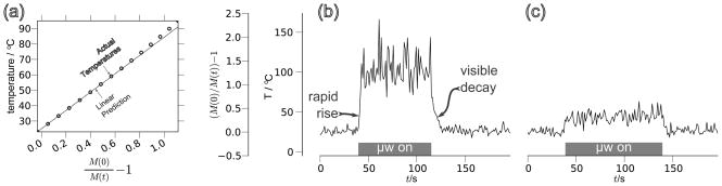
The simulated data in (a) demonstrates how the short saturation-recovery T₁ experiment can predict the temperature of the sample. The value (M(t)=M(0)) −1 is the relative difference in the observed signal, M(t). This plot assumes an initial temperature of ~ 25°C, and thus an assumed initial T_1,0 of ~ 2.5 s. The time-dependent response of the heating while cycling the microwave power from off to on is presented for both for (b) a sample positioned inside an ENDOR cavity as well as (c) inside the previously described home-built (“open-bottom”) probe design [8, 17, 33]. Both probes operate with an NMR resonance frequency near 15 MHz.

One can also use this experiment to quickly test the performance of ODNP probe configurations. Since a commercially designed ENDOR cavity has a built-in rf coil, we expected that it might present less perturbation of the electric field in the cavity and so demonstrate either less sample heating or a significantly faster temperature response than a home-built design. Surprisingly, a home-built ODNP probe of the modular design previously used for publications by the Han lab (the “open-bottom design” as in [33], see Appendix B) performed better overall, with a lower sample temperature that responds on a similar or faster timescale than in the case of the ENDOR cavity (Fig. 4).

Like others (e.g. [3, 33]), we initially assumed that the transfer of heat through the capillary wall does not vary significantly between different probes and hardware setups. However, we now believe the home-built setup exhibits less net heating because only a single layer of quartz separates the cooling air and the sample, while in the ENDOR setup, two layers of quartz are present (the sample capillary wall and the wall of the outer capillary used for positioning), and thus an intermediate, insulating layer of air comes between the cooling air and the sample. Thus, heat dissipation should be carefully considered when designing an ODNP probe.

We present a new ODNP probe in which the NMR probe and sample are contained inside a 3 mm quartz tube that passes entirely through the top and bottom openings of the microwave cavity (“pass-through design”) [94, 95], while retaining the same sample size of 3.5 μL and a design that any standard high-sensitivity cw ESR cavity can accommodate. Air flows through the 3 mm quartz tube, and thus over and across the NMR coil and sample capillary (0.6 mm i.d. 0.84 mm o.d. quartz, for both designs), resulting in more consistent sample cooling. Further comparison and contrast of the new “pass-through” and the previously presented [8, 17, 33] “open-bottom” designs are given in Appendix B.

Next, the more accurate inversion-recovery sequence measured the T_1,0 time of water as a function of incident microwave power in order to compare the new pass-through probe design to the open-bottom probe design. The Hindman model (Fig. 2) can then determine the sample temperature from the value of T_1,0 (Fig. 5) at each microwave power increment [96]. Upon removing and reinserting the NMR probe, as well as upon changing the cavity matching, we find (not shown here) that the sample temperature in the open-bottom design can vary dramatically. In contrast, the dependence of temperature on microwave power in the improved pass-through probe design is reproducible and smaller overall. Both the more accurate positioning of the sample in the area of minimal electric field and the more consistent air cooling contribute to the improved performance of the pass-through probe (cf. Fig. 5). The consistent rate of sample heating provided by the new pass-through design (i.e. reproducible ΔT_1,0) proves more critical, as reproducible heating effects can be systematically corrected for by tracking the change in T_1,0 as a function of power, as will be shown in Section 5.4.

Figure 5.

A series of experiments show how the T_1,0 of pure water increases with increasing microwave power for two different hardware setups. The model of Fig. 2 (from [56]) then converts the T_1,0 values to temperatures (y–axis on the right). The solid lines give a linear regression fit for the variation of the T_1,0 as a function of temperature.

5.3. Consensus Coupling Factor for Bulk Water

5.3.1. Observation of Enhancements

We first present a select set of ODNP enhancements for 4-hydroxy-TEMPO spin probes freely dissolved in water. At a concentration of 100 mM, where k_ρCT_1,0 ~ 100 ≫ 1, we expect the leakage factor to remain approximately constant with power. Thus, the uncorrected model (Eq. (12)) reasonably fits to the enhancement values. These approach a maximal enhancement, E_max, of −204 at high microwave power. This E_max value agrees reasonably with recent literature data that draws from pulsed ESR and FCR measurements [3], while significantly exceeding previous predictions gleaned from cw ODNP measurements [17].

Eq. (32) predicts that the enhancements observed at higher microwave power for low concentration samples will present an approximately linear dependence on the microwave power, rather than approaching an asymptotic limit, i.e. they should deviate significantly from the uncorrected model (Eq. (12)). To test this prediction, we acquired the enhancement vs. microwave power, E(p), curves for 10 μM, 150 μM, and 1.5 mM concentration solutions of 4-hydroxy-TEMPO (Fig. 6). For all experiments, the repetition delay, t_rd, between NMR scans satisfies t_rd > 5T_1,max (see Eq. (37)), while the dense, linear sampling of data points plays a critical role in clearly identifying the misfit to the uncorrected model that occurs at lower concentrations. For samples with 150 μM spin probe concentration and lower (where k_ρCT_1,0 ≤ 0.15 ≪ 1 cf. Eq. (32)), even the best fit to the uncorrected model (Fig. 6b) deviates significantly from the E(p) values. These results show that the value of E_max is not useful for a rigorous analysis of the hydration dynamics at lower spin probe concentrations. Instead, it is possible to accurately determine the value of k_σs_max, as we will show in Section 5.4.

Figure 6.

ODNP signal enhancement, E(p), as a function of power, p, for four different concentrations of 4-hydroxy-TEMPO spin probes dissolved in water. We integrate the enhanced signal intensity and normalize it against the unenhanced signal intensity (i.e. E(0) = 1) in order to determine the unitless value of E displayed along the y–axis. The solid lines show the best fit to the uncorrected model (Eq. (12)). The spectrometer acquires the black points in order of increasing microwave power; to check for reproducibility (e.g. lack of sample loss during the experiment), it then acquires the red (gray) points in order of decreasing microwave power.

5.3.2. Measuring the Consensus Coupling Factor

The measurement of ξ for a solution of small spin probes freely dissolved in bulk water is crucial for extracting D_local. In order to measure this “bulk coupling factor” (i.e. ξ between a small spin probe and the bulk water nearby), with cw ODNP, one must measure ξs_max(C) over a range of concentrations. One can then extrapolate the value of s_max given by Eq. (17) to the low concentration and/or high concentration limit(s), where s_max → 1/3 and s_max → 1, respectively [17, 28]. The study by Armstrong and Han [17] obtained a ξ of 0.22 by extrapolating a relatively evenly spaced series of concentrations between 0 and 15 mM. These measurements covered a lower concentration range than studies by Türke and Bennati that report a higher coupling factor of 0.32–0.33 for 5, 10, and 25 mM solutions [30]. Basic calculations can rule out the possibility that, at low spin probe concentrations, the bulk water does not completely diffusively exchange with the water near the spin probe on a timescale less than the NMR T₁ time. Therefore, we carefully re-measure the value of ξs_max over a wider range of concentrations, both low and high, in order to quantify the bulk water coupling factor, ξ.

Fig. 7 presents ξs_max(C) for 4-hydroxy-TEMPO solutions ranging from 10 μM to 100 mM concentrations. At this point, we are not yet considering strategies to correct for microwave heating effects. Therefore, the uncorrected model (Eq. (14)), which assumes a constant leakage factor for all microwave powers, was used to calculate all the data presented in this figure. However, within this context, we calculate the leakage factor in two ways; for clarity, we distinguish the two by denoting them as f* vs f^†.

Figure 7.

Measurement of ξs_max(C), the product of the maximal saturation factor (which varies with concentration) and the coupling factor (which is constant with concentration), over a wide range of spin probe concentrations, C. We compare ξ^*s_max(C), which follows the previously standard method for determining the coupling factor, to ξ^†s_max(C), where we calculate the NMR self-relaxivity (k_ρ), and therefore the leakage factor, f^†, exclusively from accurate high-concentration data. We show that the values of ξ^†s_max(C) have far less scatter than the values of ξ*s_max(C). As a result, we can compare this to the function ξs_max(C) = 0.33 × 2/(3 + 3b″) (shown as a solid gray line), where s_max(C) is given by Eq. (17) and the values of b″/C and ξ = 0.32 – 0.33 have been previously reported by Türke and Bennati based on the results of pulsed ESR measurements on ¹⁵N 4-hydroxy- TEMPO [30]. Though this line matches well to the data presented here, it is determined exclusively from the measurements in [30]. A threshold was applied to the ξ*s_max data to keep values plotted here within the allowed range of 0 ≤ ξs_max ≤ 0.5; thus, the data for the points shown lying at the limits of the y-axis actually fall outside the allowed range.

First, we employ the conventional method for determining the leakage factor from f*(C) = 1 − T₁(C)/T_1,0 (Eq. (10)), where each f*(C) is derived from an independent measurement of the NMR T₁(C) time at each concentration, C. As previously discussed in Section 4.4, the resulting value of ξ*s_max = (1 − E_max)/f* is ill-determined at low concentrations where f* → 0. Therefore, the resulting data has high scatter at low concentration, leading to many outliers, some of which have such high errors that they exceed the physically plausible range of 0 ≤ ξ* ≤ 0.5 set for dipolar interactions [1]. Fortunately, we can more accurately determine these values with an alternative approach – these are denoted as ξ^†s_max(C).

Following a recommendation from Section 4.4, we calculate $f^{†}=k_{\rho }C/(k_{\rho }C+T_{1,0,0}^{-1})$ (Eq. (8)) from a single, accurately measured value of k_ρ. This value is calculated (using Eq. (36)) exclusively from 100 mM solutions of spin probe, where the self-relaxation rate due to the spin probe (k_ρC) is very large/fast and therefore easily quantified. As shown in Fig. 7, the resulting ξ^†s_max values present a dramatically reduced scatter (where ${\xi }^{†}{s}_{\mathit{max}}(C)=(1-E_{\mathit{max}})/f=(1-E_{\mathit{max}})(k_{\rho }C+T_{1,0,0}^{-1})/k_{\rho }C$). We see a clear and meaningful trend in ξ^†s_max(C), even for concentrations as low as 10 M. This trend matches the predictions of Bennati and coworkers [30, 58] (represented in Fig. 7 as a grey solid line) and therefore concurs with their measured value of ξ_bulk = 0.32 − 0.33, rather than the previously measured value ξ_bulk = 0.22 ([17]), as a representative result for a bulk water coupling factor measurement that has not yet been corrected for heating effects. The result previously measured by Armstrong and Han [17] (i.e. ξ_bulk = 0.22) is likely affected by the presence of the artifact arising from the significant lengthening of T_1,0 with microwave power, especially since the concentration series in [17] was measured over a lower range of concentrations (≤ 15 mM), where the lengthening of T_1,max is more pronounced than at higher concentrations (Eq. (37)).

Contrary to conclusions drawn in previous literature [30, 71], these new results confirm that only cw ODNP methods can provide quantitative and accurate coupling factors and, thus, derive accurate hydration dynamics information. This is the case even down to 10 μM concentrations. This is fortuitous; FCR and pulsed ESR tools will continue to present powerful and complementary capabilities, while the implementation of quantitative ODNP measurements on widely available and easy to use cw ESR instrumentation has distinctly practical benefits for the end user. Having come to a consensus with other recent publications [3, 30] in that the value of the bulk coupling factor is indeed measured as ${\xi }_{\mathit{bulk}}^{†}=0.32-0.33$ before any heating correction is applied, this allows us to move forward and correct for the heating-induced variation of relaxation times.

5.4. Application of the Corrected Model

5.4.1. Measurement of Relaxation times

In order to apply the corrected analysis, we must first acquire the NMR relaxation rate, $T_1^{-1}(p)$, as a function of power. We do this, and also compare it to the bulk water relaxation rate, $T_{1,0}^{-1}(p)$. This first allows us to calculate the variation of the leakage factor with microwave power, $f(p)=k_{\rho }C/T_1^{-1}(p)$, for different spin probe concentrations. At low spin probe concentration, the leakage factor varies significantly, exhibiting an approximately linear dependence on microwave power (as predicted by Eq. (32)). In contrast, at high spin probe concentrations (e.g. 100 mM), the leakage factor (f(p, C)) does not vary significantly, since it has a value of f ≈ 1 for all microwave powers, which is why the high concentration samples yield close adherence even to the uncorrected model (Fig. 6). The self-relaxation rate, k_ρC, (Table 2) is the difference between the total relaxation rate, $T_1^{-1}(p)$, and the bulk water relaxation rate, $T_{1,0}^{-1}(p)$, (following Eq. (29)), and it graphically appears in Fig. 8 as the distance between the two respective lines (black arrow).

At low spin probe concentrations (< 2 mM), the variation in k_ρC with temperature is insignificant relative to the sizable variation in the bulk water relaxation rate, $T_{1,0}^{-1}(p)$ (see the slope of $T_{1,0}^{-1}$ vs power for 10 μM–1.25 mM in Fig. 8). Similarly, the next section will demonstrate that k_σ likewise does not vary significantly. These observations are surprising. The traditional viewpoint [1, 3], holds that the dynamic dependence of the ODNP signal is quantified by the coupling factor, ξ = k_σ/k_ρ, not by T_1,0 or f (p, C). Based on this, one would intuitively assume (as in [58]) that changes in temperature would primarily induce changes in ξ. However, the observations here emphasize the fact that while ξ does indeed quantify local water dynamics, T_1,0(p), and therefore f(p, C), also include contributions from bulk water dynamics. Furthermore, as we know from the Hindman model (Fig. 2), the T_1,0 time responds very sensitively to changes in bulk dynamics. As a result, especially at lower concentrations (≤ 500 μM) of nitroxide probes, the heating-induced variations in the relaxivities, k_σ and k_ρ, that encode the local dynamic information play a far less important role in determining the ODNP signal enhancements than heating-induced variation in the bulk water relaxation, $T_{1,0}^{-1}$. In contrast, at high concentrations, the $T_{1,0}^{-1}$ rate forms a relatively insignificant contribution to the net $T_1^{-1}$ relaxation rate (see $T_1^{-1}$ vs T_1,0 for 100 mM in Fig. 8), which is dominated by k_ρC.

5.4.2. Measurement of k_σ and ξ

A typical uncorrected analysis (as presented in the previous section) employs the E(p) curves and E_max values (as shown in Fig. 6) directly to calculate the hydration dynamics via Eq. (14). However, in preparation for employing the corrected analysis, Fig. 9 displays the uncorrected analog of k_σs(p), i.e.

Figure 9.

Microwave power dependence of the product of the cross-relaxation with the electron saturation factor, i.e. k_σs(p), for the same series of experiments as Fig. 6. The uncorrected curves (blue empty circles and dashed curves) present (1 – E(p))/CT₁(0)659.33 and so have the same shape as the curves in Fig. 6 (though inverted); as explained in the text, these are only apparent values, i.e. $k_{\sigma }{s}_{\mathit{eff}}^{\ast }(p)$. The solid black curves and filled black circles present the k_σs(p) product, as determined by the corrected analysis (i.e. (1 – E(p))/CT₁(p)659.33 as determined by Eqs. (39) and (42).

$$k_{\sigma }{s}_{\mathit{eff}}^{\ast }(p)=\frac{1-E(p)}{C{T}_1(0)659.33},$$ (44)

which extrapolates to

$$k_{\sigma }{s}_{\mathit{max},\mathit{eff}}^{\ast }=\frac{1-E_{\mathit{max}}}{C{T}_1(0)659.33},$$

where $s_{\mathit{max},\mathit{eff}}^{\ast }$ is defined by Eq. (35). The corrected values of k_σs(p) differ from $k_{\sigma }{s}_{\mathit{eff}}^{\ast }(p)$ simply by including the power variation of T₁(p), i.e. substituting T₁(0) → T₁(p) in Eq. (44). The interpolated (via Eq. (39)) values of T₁(p) used for this purposes are the same as those shown by the solid line in Fig. 8.

The k_σs(p) data generated from the corrected model (Eqs. (42) and (43)) now indeed visibly level off at high microwave power (Fig. 9a–b, solid line), indicating that the highest microwave powers employed in this study significantly saturate the ESR transition. This is the first time ODNP data has displayed a stable and consistent saturation (as predicted by Eq. (11)) that extends over several microwave power increments. The higher concentration data shown here do not level off simply because the ESR transitions requires the application of more intense microwave radiation before they saturate appreciably (i.e. p_1/2 is greater as a result of the fast Heisenberg exchange and subsequently broader ESR linewidth). The values of k_σs_max are different at different concentrations because s_max remains closer to 1/3 at low concentration, while Heisenberg exchange drives s_max close to 1 at high concentrations.

The differences between the uncorrected ( $k_{\sigma }{s}_{\mathit{eff}}^{\ast }(p)$) and corrected values of the k_σs(p) data (as shown in Fig. 9) lead to several improvements. These improvements are most apparent at lower spin probe concentrations and at higher microwave powers. The corrected model accounts for a significant change in T₁(p)⁻¹ with microwave power (as shown in Fig. 8) thus removing the dependence of $s_{\mathit{eff}}^{\ast }(p)$ on ΔT_1,0 (Eq. (34)). As the value of ΔT_1,0 can change with changes to the hardware setup, removing this dependence should make the measured value of k_σs_max more reproducible than the measured value of $k_{\sigma }{s}_{\mathit{max},\mathit{eff}}^{\ast }$. Also, as the corrected values of k_σs(p) fit much more closely to the corrected model than the values of $k_{\sigma }{s}_{\mathit{eff}}^{\ast }(p)$ fit to the uncorrected model, the fitting error is dramatically reduced. Thus, when the corrected k_σs(p) values are extrapolated to infinite power, more accurate values for k_σs_max and, therefore, the coupling factor, ξ, are obtained.

Interestingly, the fact that all the data fit well to the corrected model implies that k_σ does not vary significantly as a function of microwave power under the experimental conditions employed here. Obviously, when more advanced instrumentation and measurements allow one to distinguish much more subtle changes in relaxivity, or with uniquely temperature sensitive systems, one may wish to revisit variation of k_σ with microwave power as a secondary correction [97].

Table 3 summarizes the numerical results for the four representative 4-hydroxy-TEMPO spin probe concentrations shown in Fig. 9. For the sake of completeness, we also show the results when attempting to calculate a value of ξ*, where k_ρ is determined from low concentration data; as shown before (Section 5.3.2), these values are highly scattered, again emphasizing the necessity for obtaining k_ρ from higher concentration data or from larger samples, both of which yield higher signal to noise. The values of s_max given in Table 3 are calculated via. Eq. (17), with b″/C = 198.7 M⁻¹. As mentioned before, the uncorrected values of the coupling factor agrees with the values of Türke and Bennati [30] (ξ_bulk = 0.32–0.33), as well as the values predicted by FCR [8, 58] and MD simulations [34]. However, the corrected values approach a number closer to ξ_bulk = 0.27. We should note that additional experiments (data not shown) were done to verify that we choose a field relative to the cavity frequency that is positioned exactly on the ESR resonance (i.e. the field that maximizes p_1/2). The error analysis of the fitting procedure is complex [98], and will be the subject of future investigations.

Table 3.

Values of the cross relaxivity, self relaxivity, and coupling factor for the dipolar interaction between water and free spin probes at ambient temperature, measured at four representative 4-hydroxy-TEMPO spin probe concentrations. The numbers in italics and parentheses present the inaccurate values that result from attempting to calculate k_ρ from samples with very low concentrations of spin probe (i.e. where Eq. (36) has a significant error), leading to an apparent coupling factor of ξ*. We calculate a value of ξ (and ξ*) both with and without the correction for the change in the T₁(p) times as a function of power (as given by Eq. (42) and Fig. 9), labeled as “corrected” and “uncorrected,” respectively. (The analysis of uncorrected value of ξ* is equivalent to that of Section 5.3.2, while the analysis of the uncorrected value of ξ is equivalent to ξ^† of Section 5.3.2.)

	10 μM		150 μM
	uncorrected	corrected	uncorrected	corrected
kσsmax/s−1M−1	42	34 ± 1.3	37	32 ± 1.6
smax[30, 31]	—- 0.334 —-		—- 0.352 —-
kσ	126	102	105	91
kρ/s−1M−1	—- (−137) 353.4 —-		—- (391) 353.4 —-
ξ	0.36	0.29	0.30	0.26
ξ*	(−0.94)	(−0.74)	(0.27)	(0.23)
τc,bulk/ps	26	47	44	59
	1.25 mM		100 mM
	uncorrected	corrected	uncorrected	corrected
kσsmax/s−1M−1	50	43 ± 1.3	112	89.8 ± 10
smax[30, 31]	—- 0.465 —-		—- 0.968 —-
kσ	107	92.7	116	92.8
kρ/s−1M−1	—- (357) 353.4 —-		—- 353.4 —-
ξ	0.31	0.26	0.33	0.26
ξ*	(0.30)	(0.26)	(0.33)	(0.26)
τc,bulk/ps	40	58	34	58

5.4.3. Corrected Measurement of the Coupling Factor

We can now finalize the discussion on the coupling factor associated with bulk water, ξ_bulk. We present data over a large range, from low concentration (10 μM) for which s_max = 1/3 to high concentration(> 100 mM) for which s_max approaches 1, shown in Fig. 10. To test for reproducibility, data was collected at two different air flow rates (14 vs 20 SCFH or 6.6 vs 9.4 L/min) that do show different results when analyzed with the uncorrected analysis. The data shows not only a good match to the Heisenberg exchange model (Eq. (17)) for ξs_max(C) but significantly covers a wide range of biologically relevant concentrations of 10–500 μM. From this curve, after accounting for the varying s_max values, we find ξ_bulk = 0.27 (which corresponds to τ_c,bulk = 54 ps). The scatter resulting from the use of different flow rates is insignificant, as the model corrects for the variable heating effect.

Figure 10.

Values for ξs_max(C) (the product of the coupling factor and the maximal saturation factor) extracted with the corrected model over a wide range of concentrations. As in Fig. 7, the solid curve gives the values predicted for ξs_max(C), still employing b″/C = 198.7 M⁻¹, but now with a value of ξ = 0.27. The data shown are taken at two different flow rates: 14 SCFH=6.6 L/min (filled circles) and 20 SCFH=9.4 L/min (filled diamonds). The unfilled symbols give the value of ξ^†s_max(C) calculated from the same data, but without the heating correction (i.e. assuming T₁(p) = T₁(0) for all T₁(p)).

For future measurements, the corrected model should be applied and the corrected value of ξ_bulk = 0.27 (and τ_c,bulk = 54 ps) used to extract a value for D_local (Eq. (20)). However, it is some-times not practically feasible to use the corrected model, i.e. for re-analyzing data in previous studies where no T₁(p) measurements were acquired. For such cases, we note that the heating effect leads to a systematic elevation of the measured coupling factor. Thus, as applies to virtually all published data to date, in order to estimate the value of D_local, it is best to compare the uncorrected coupling factors to ξ_bulk = 0.32 – 0.33 and τ_c,bulk=36.4 ps – 33.3 ps.

5.4.4. Outlook to 100 M and Lower: Biological Samples with Tethered Spin Probes

An example of an application of the new analysis to biomolecular systems helps to clarify the importance of the preceding results. We selected 200 nm diameter unilamellar vesicles made of DOPC lipid (18:1 (Δ9-Cis) PC, i.e. 1,2-dioleoyl-sn-glycero-3-phosphocholine, Avanti Polar Lipids #850375), dissolved in water at two different concentrations: 4.89 mM and 32.0 mM. An inversion recovery experiment determined the values of T_1,0,0 for the sample at these two concentrations. For the ODNP E(p) and T₁(p) measurements, we prepared another pair of samples that also includes 3 mole % of a spin labeled lipid (16:0 Tempo PC, i.e. 1,2-dipalmitoyl-sn-glycero-3-phospho(tempo)choline, Avanti Polar Lipids #810606) that contains a nitroxide probe tethered at the surface of the lipid bilayer. The final spin probe concentrations in these samples were 150 μM and 960 μM.

Despite the similar appearance of the two lines in Fig. 11, the 32 mM sample does indeed exhibit much higher enhancement values (E_max ≈ −20) than the diluted sample (E_max ≈ −4.9). However, they converge to similar values of k_σs(p) (Eq. (42)), yielding k_σs_max values of 19.6 and 19.5, respectively.

Figure 11.

Shows implementation of the corrected model on an ODNP measurement of k_σs(p) at different values of the microwave power, taken for a mixture of tethered TEMPO label (3% mole ratio) embedded in a DOPC lipid. The values shown are measured from solutions containing 32.0 mM lipids (circles) and 4.89 mM lipids (open triangles), with 960 μM and 150 μM of spin probe, respectively. The values plotted here are scaled by the T₁, following Eq. (42). For clarity, we have omitted the best fit lines for the uncorrected data, $k_{\sigma }{s}_{\mathit{eff}}^{\ast }(p)$, in blue; as we also observed for free spin probe samples, this data does not fit well to the asymptotic model.

As previously reviewed, spin probes tethered to such large biomolecular systems tend to give results that one can interpret more readily than those for freely dissolved spin probes, since the nitrogen relaxation drives s_max to closely approach 1 ([17]), yielding k_σs_max ≈ k_σ. At the same time, this motional restriction also typically causes tethered spin probes to exhibit a faster ESR relaxation time than untethered spin probes and thus makes the ESR transitions harder to saturate. For instance, while k_σs(p) for a free spin probe of 150 μM concentration in Fig. 9b (Sections 5.3.1 and 5.4.1) begins to level off near 1 W of microwave output power, the k_σs(p) values for the 4.89 mM sample of DOPC, which have the same probe concentration of 150 μM, do not begin to saturate until the highest powers of ~3 W are applied, as presented in Fig. 11. The requirement for such high powers can lead to rather significant heating effects, making it even more important to use the corrected model to quantitatively determine the coupling factor. In the case of the DOPC sample, we observe an uncorrected value of k_σs_max that differs from the corrected value by more than 18%. (The best fit values for the uncorrected $k_{\sigma }{s}_{\mathit{max},\mathit{eff}}^{\ast }$ shown in Fig. 11 are 24.5 s⁻¹M⁻¹ for the 32 mM DOPC sample and 23.2 s⁻¹M⁻¹ for the 4.89 mM DOPC sample.)

Eq. (36) can compare the T₁ times in the absence of microwave power (i.e. T₁(0) and T_1,0,0, respectively) for the labeled and unlabeled 32 mM samples, yielding k_ρ = 314s⁻¹M⁻¹. Then, we can calculate the coupling factor from Eq. (3) (ξ = k_σ/k_ρ), and convert it to a correlation time, τ_c,site as previously reviewed. In general, we expect the uncorrected value of τ_c,site to be systematically shorter. Indeed, the corrected model extracts a value of τ_c,site of 264 ps, while the uncorrected value is more than 14% shorter. Eq. (20) can compare these to the corrected (54 ps) and uncorrected (33.3 ps) values for the bulk water correlation time, τ_c,bulk, calculating the local diffusion coefficient on the surface of the DOPC to be 3.98 × 10⁻¹⁰ m²s⁻¹ if the uncorrected model is used and 5.52×10⁻¹⁰ m²s⁻¹ if the corrected model is used (Eq. (20)). Thus, interestingly, the corrected value of D_local is actually 30% faster than the uncorrected value.

Finally, we note that even with the corrected analysis, it is necessary to be cautious with systems where the small residual changes in temperature with increasing microwave power might induce a transition in the structure and dynamics (such as macromolecules that undergo a glass transition [99, 100], or proteins that undergo aggregation [12], folding, or unfolding [10]) to insure that the transition temperature does not fall between room temperature and the temperature at the maximum microwave power (≈ 35°C). In such cases, the corrected model will present an advantage by more effectively registering and highlighting any sudden changes in k_ρ and/or k_σ (and therefore ξ) as an unexpected change in k_σs(p) or T₁(p) with increasing microwave power, p.

5.4.5. The Corrected Analysis in Context

The retardation of the local translational diffusion dynamics, relative to those in bulk, is an important parameter of biophysical significance. Therefore, we now ask how the results presented here, and the use of the corrected model in particular, will broadly affect the determination of the local translational diffusion coefficient of water, D_local. In order to extract D_local with ODNP, one needs to accurately determine both the translational correlation time for the interaction between freely dissolved spin probes and bulk water, τ_c,bulk, as well as the correlation time at the spin labeled site of interest, τ_c,site. (As previously discussed, these are typically determined from FFHS analysis of the associated ξ_bulk and ξ_site values, respectively.) Thus, the results that have been presented here can affect the quantitative values of D_local in two ways, following Eq. (20). First, choosing the longer, corrected reference value of τ_c,bulk = 54 ps will increase the resulting value of D_local. Second, the corrected model will yield a different value of τ_c,site than the uncorrected model.

Given the potential controversy over the bulk coupling factor, many ODNP studies in the literature anticipated such a dilemma in reporting on the absolute values for D_local. For this reason, they reported only the translational correlation times, τ_c,site, which do not depend on the bulk water coupling factor, or they reported results based on the consensus value of ξ_bulk = 0.33 [9].

Of course, for a given measurement, the extent to which heating effects affect the final value of τ_c,site that the uncorrected model reports will depend on the details of the hardware (which control ΔT_1,0) as well as the T₁(0) and T_1,0,0 of the sample. Therefore, changes in these parameters could potentially result in scatter in the final τ_c,site values. However, previous publications reproducibly employ measurements of τ_c,site to identify meaningful and biologically significant trends and transitions associated with changes in the local hydration dynamics [9, 10, 12, 15, 16, 20, 99–103]. The level of accuracy with which these publications identified such trends was achieved by only comparing τ_c,site values that come from the same dataset, i.e. from enhancement data acquired both over the same sampling of microwave powers and also from similar samples positioned in precisely the same position of the same cavity. Thus, in these previous measurements, the heating effects are systematic and the qualitative trends and comparisons of ξ_site, τ_c,site, and D_local within each dataset remain accurate. However, we would like to estimate an upper limit on the heating-induced error between different datasets, where experimental conditions might vary slightly. Therefore, we next collect the results from several of such previous studies.

We find that we can sort the resulting collection of measurements into four categories (Fig. 12). With the exception of the polyelectrolyte hyaluronic acid, which exhibits very fast surface hydration dynamics [9], bulk water is the only sample so far that has presented a τ_c,site < 120 ps. Thus, we can classify this regime as “bulk-like,” i.e. significantly faster than the hydration dynamics observed near most macromolecular compounds. Researchers have routinely observed values of 120 ps < τ_c,site < 225 ps for the dynamics of the hydration water surrounding macromolecular systems, including unfolded proteins, polyelectrolytes, and polymers, as well as the surface of lipid vesicles and folded globular proteins [9, 10, 20, 99, 100, 104]; we denote this regime as consistent with “surface” dynamics. Similarly, the “buried” regime includes values of τ_c,site > 340 ps. In this regime, researchers have observed slow water permeating past spin labeled sites that are expected to be buried inside a macromolecular complex, such as complexed polyelectrolytes [9, 104], aggregated protein fibrils [9, 12], buried sites of natively folded and molten globule states of ApoMb [10], and lipid vesicles where the spin probe is attached 14 bonds deep into the vesicle (i.e. 14 Doxyl PC) [99, 100]. Finally, we denote an “intermediate” regime of 225 ps < τ_c,site < 340 ps, which includes most samples where one intuitively expects hydration water to exhibit dynamics intermediate between the buried and surface regimes, including surface labeled lipid vesicles in the presence of viscogens such as 20% PEG [9] or binding agents such as ≥ 35 μM P188 [100], lipid vesicles with spin probes attached at the carbon positions immersed five to ten C-C bonds into the lipid bilayer (i.e. for label molecules 10 Doxyl PC, 7 Doxyl PC, and 5 Doxyl PC) [99], and the surface of the partially folded molten globule state of ApoMb [10].

Figure 12.

Data for the coupling factor, ξ, between a spin probe attached to specific, known biological sites and the nearby (within 0.5–1.5 nm) hydration water, collected from a recent series of publications [9, 10, 12, 99, 100, 104]. All data shown therefore employs the uncorrected model to extract ξ. The retardation factor τ_c/τ_c,bulk = D_H2O/D_local gives the slow-down of the translational hydration dynamics relative to bulk water; the measurement for τ_c,bulk sets the value of 1 on the retardation axis and, therefore, for the absolute values of the diffusivities. Both the consensus value (at τ_c/τ_c,bulk = 1) and the previously employed value (at τ_c/τ_c,bulk = 2.3) are shown above with a blue “x”. Of course, if the previously employed value were used to set the value of 1 on the retardation axis, the value of the diffusion would change for all the data points shows. For comparison, the bottom inset shows the same FFHS curve plotted over a larger range of logarithmically spaced correlation times.

In summary, even though these data come from previous studies that employ the uncorrected model for analysis, the value of the correlation time (and coupling factor) that each study determines reproducibly fall within a particular zone corresponding to the spin probe location (i.e. exposed, intermediate, or buried). There are few exceptions to this trend, regardless of whether the site resides on a protein, membrane vesicle, or polymer (Fig. 12). Lipid vesicle samples admixed with doxylstearic acid labels are a notable exception; these data are not shown since they consistently show higher dynamics than their tempo-PC analogs (which are presented in this plot). Also, despite its unfolded conformation, the protein mfp151 [9] also exhibits buried-like dynamics, and because of this is believed to have partial local structure near the spin labeled site [9], while the native (i.e. folded) state V66R1 site in ApoMb (Apomyoglobin) [10] exhibits intermediate dynamics, even though it is believed to be on the surface of the protein, which is likely due to specific local surface topology or chemistry. It is worth noting that most datasets reviewed here are acquired with the same microwave cavity and NMR probe design and come from samples with relatively high, ≥ 500 μM, spin probe concentrations. However, the relatively strict adherence to this classification scheme indicates that the level of precision of ODNP is already fairly high before utilizing the corrected model. Specifically, when one analyzes ODNP data with the uncorrected model under similar conditions, one can compare to previously acquired, independent datasets with at least the level of resolution needed to discriminate the different translational diffusion rates of water as it moves past surface vs intermediate vs buried macromolecular sites.

Previous research suggests that changes in the surface hydration dynamics should correlate strongly with the interfacial forces that drive biological and polymeric transitions [50, 83, 105–107]. Interesting effects, such as protein folding and complexation, initiate at sites with “intermediate”-regime hydration dynamics. This has been seen for both the ApoMb [10] and vesicle [100] data. Therefore, despite the detailed level of reproducible resolution the uncorrected analysis already gives us, a particular interest in performing more highly resolved studies of the rich variation of the hydration dynamics within the “intermediate” regime compels us to explore the potential benefits of extracting more accurate values of D_local with the corrected model.

In the previous section, we noted a 30% increase in the measured value of D_local when all data was analyzed with the corrected model. This improvement in the accuracy of D_local (i.e. change in absolute value) is dominated by the switch to the corrected reference value of τ_c,bulk (derived from ξ_bulk = 0.27), which is 47% longer than the uncorrected value (derived from ξ_bulk = 0.33). This is partially compensated by the fact that we also expect τ_c,site for the sample of interest to be systematically longer (i.e. slower). Therefore, a systematic correction of only ~ +30% in D_local seems likely. In addition to this systematic correction, by removing any dependence on ΔT_1,0, the corrected analysis should also allow one to accurately and reproducibly improve the precision of ξ_site, τ_c,site, and, therefore, D_local across different protocols and instruments (see Section 5.4.3 for a dramatic demonstration). Importantly, the corrected analysis will not only allow one to report values on an absolute scale more confidently, but will also dramatically increase the resolution of the dynamic timescales that one can resolve and compare between different datasets, allowing one to explore and reproducibly classify finely resolved dynamic sub-regimes.

6. Conclusions

After presenting our review of existing methods, we identified and targeted what we view as the most essential bottlenecks to advancing ODNP as a tool for characterizing hydration water. The resulting corrected model and analysis, proposed here (Eqs. (42) and (43)), present a significant improvement in the ability of cw ODNP to accurately quantify hydration dynamics. It is the first model to fit accurately acquired (i.e. without artifacts) enhancement vs. power (E(p)) data for low (≤ 500 μM) concentrations of spin probes. The data also resolves the debate over the determination of the bulk water coupling factor, pointing out that the higher value proposed in recent years (0.30, 0.32–0.33, 0.33–0.35, and 0.36 from [34], [30], [58], and [8] respectively), rather than one previously determined by cw ODNP (0.22, from [8]) is the value expected for measurements extracted without any heating correction. Going one step further and improving the accuracy of the data analysis by accounting for the effect of the small residual microwave heating on the bulk NMR relaxation time leads to a corrected value of ξ_bulk = 0.27 and τ_c,bulk = 54 ps. We have discussed how implementing this correction for all ODNP measurements should systematically improve the absolute value of the measured local diffusivity, D_local, by approximately 30%, while also eliminating discrepancies (scatter) between independent datasets that might be as high as 5–10%, thus permitting an overall more accurate and precise measurement, and a subsequently more refined and reproducible classification of hydration dynamics. We validate the experimental strategy proposed in [8] that solely cw ODNP hardware is a viable quantitative analytical tool for determining the coupling factor, ξ, albeit now with corrected numbers. This conclusion is particularly promising and advantageous to the ODNP and analytical biochemistry communities since cw ODNP hardware requires significantly less user training and expenditure than pulsed ESR hardware, and thus is more broadly available.

Five clear conclusions dominate this presentation: (1) by measuring the bulk water relaxivity, one can intrinsically probe the sample temperature and thus develop the next generation of cw ODNP hardware; (2) by measuring and accounting for T_1,max, one can acquire reproducible signal enhancement data for a particular system; (3) by analyzing data with the new model presented here, one can recover accurate values of ξ, even in the presence of moderate sample heating; (4) by carefully repeating measurements over a range of concentrations, cw ODNP can retrieve values of the bulk coupling factor that do indeed agree with predictions given by pulsed ESR and FCR measurements taken at similar concentrations; and (5) by independently measuring k_σ, one can access information about the translational dynamics, even at concentrations of down to ten micro-molar, opening up opportunities to study a wide range of new systems of biological significance.

For future development of new NMR probes and/or ESR cavities, we can also specifically suggest that cw ODNP analysis of ≤ 150 μM 4-hydroxy-TEMPO gives a complete test of the hardware’s performance. The enhancements and relaxation times of such low concentration systems change significantly and clearly indicate any heating effects (as in Fig. 6a). Since lower concentration samples saturate easily, one can also easily observe the power where the corrected k_σs(p) curve (e.g. Fig. 9) derived from the same data flattens out – this is proportional to the value of p_1/2 (see Eq. (11)), which can also be used to characterize the hardware performance. Specifically, in the typical case, the ratio of the field to the frequency is resonant with one of the (well-p separated) ESR transitions, so that the value of $\sqrt{1/p_{1/2}}$ gives a measure of the microwave resonator’s conversion ratio (i.e. the B₁ field generated per Watt of power transmitted into the cavity).

The results here also make it clear what comes next in the task of developing cw ODNP as an analytical tool for the quantification of local hydration dynamics. Systematic comparisons between measurements taken on different instruments or microwave cavities should now agree quantitatively. In particular, experiments that observe the change in the coupling factor across the various frequencies possible with X-band equipment would offer interesting insight into the existing models describing the hydration dynamics and should be possible with tunable cavity setups (similar extensions to the S- through Q-bands would be interesting). The results here clarify a protocol for perfectly stabilizing the sample temperature; by adjusting a cryostat differently at different microwave powers to ensure a consisent NMR T₁(p) time at all microwave powers, p, one also ensures a consistent sample temperature. The current study also points out the clear benefit of the development of an error analysis that properly accounts for, among others, the correlated error present in the E(p) data, as well as the development of software and hardware to more fully automate ODNP measurements. In particular, detailed error analysis could help distinguish between random measurement errors and systematic errors due to small differences in sample composition or hardware. Finally, the effort towards more consistent measurements will position the ODNP field at a point where the advances offered by theoretical methods can be tested, verified, and further developed by comparison to experimental measurements. These include comparison of data to more advanced dynamic models, such as those derived from molecular dynamics simulations [34, 69], as well as a careful re-analysis of field cycling results that deals with bulk water relaxation effects in greater detail.

Highlights.

• Overhauser Dynamic Nuclear Polarization (ODNP) can quantify the hydration water dynamics landscape with sub-nanometer locality.

• Quantitative cw ODNP measurements rely on temperature control and correction to find the correct coupling factor.

• ODNP is exploited as an unprecedented 10 GHz NMR relaxometry tool that detects the diffusion dynamics of loosely bound water.

• Previous ODNP results can be reproducibly classified into regimes of surface, interfacial vs. buried water dynamics.

Glossary

ξ

the coupling factor, an experimentally determined ODNP parameter that depends on the dynamics of water near (0.5–1.5 nm) the spin probe

cw

continuous wave

DC

direct current

DMSO

dimethyl sufoxide

DNP

dynamic nuclear polarization

DOPC

1,2-Dioleoyl-sn-glycero-3-phosphocholine

ELDOR

electron double resonance

ENDOR

electron-nuclear double resonance

ESR

electron spin resonance

FCR

field cycling relaxometry

FFHS

force-free hard sphere specifically used in ⇒ reference to a model in [47]

i.d.

inner diameter

IR

infrared

k_ρ

the local self-relaxivity (units s⁻¹M⁻¹), which gives the concentration-dependent rate of relaxation between protons near (5–10 Å) the spin probe and the bath (i.e. “lattice”)

k_σ

the local cross-relaxivity (units s⁻¹M⁻¹), which gives the concentration-dependent rate of relaxation between protons near (5–10 Å) the spin probe and the electron spin of the spin probe

MD

molecular dynamics

MR

magnetic resonance

NMR

nuclear magnetic resonance

o.d.

outer diameter

ODNP

Overhauser effect dynamic nuclear polarization

PC

phosphocholine

PEG

polyethylene glycol (i.e. poly(oxyethylene))

rf

radio frequency

SL

spin label, i.e., spin probe

spin probe

molecules or moieties containing unpaired electron spins

T₁

the NMR longitudinal relaxation time for a sample with spin probe incorporated

T_1,0

the NMR longitudinal relaxation time for a sample with all spin probe removed

TE102

a rectangular microwave cavity operating in a transverse electric mode that has three coplanar electric field nodes parallel to the direction of sample insertion and perpendicular to the static magnetic field (two at the sides of the cavity) and two other planar nodes at the two sides of the cavity parallel to the static magnetic field

TEMPO

(2,2,6,6-Tetramethyl-piperidin-1-yl)oxyl

UV

ultraviolet

Appendix A

Details of Experimental Setup for Time-Resolved T₁ measurement

A numerical calculation (left pane of Fig. 4), based on the exponential T₁ decay and the Hindman model (Eq. (25)) verifies that the relative change in magnetization, (M(0)/M(T)) −1, remains a linear function of temperature, T, from 20°C to 80°C during the single-scan short-recovery T_1,0 experiments. This linear relationship relies on both the approximately linear dependence of magnetization on T_1,0 when short recovery delays are employed (here τ = 0.5 s ≪ T_1,0) and on the approximately linear dependence of T_1,0 on temperature.

We performed the single-scan short-recovery T_1,0 experiment on water loaded into a capillary and placed inside a commercial ENDOR cavity (Bruker ER 801). In this setup, variable capacitors were added inside an aluminum box outside the cavity in order to tune and match the ENDOR rf coil so it could be used for NMR signal detection. In order to position the sample in the center of the cavity, a slightly larger capillary (1.2 mm o.d.) with one fused end holds the sample capillary (0.6 mm i.d. 0.84 mm o.d. quartz). We then compared the performance of this ENDOR probe to the home-built NMR saddle-coil probe design previously described in [12, 17, 33, 100]. After loading a sample capillary into a homebuilt NMR probe, we inserted it into a typical TE102 rectangular microwave cavity and again performed the single-scan short-recovery T_1,0 experiment.

Appendix B

Pass-through vs. Open Bottom Probe Designs

In the previously described home built design (i.e. “open-bottom design”), the sample tube and rf coil protrude from an enclosed glass tube that is held in the cavity from the top, and where the cooling air enters the cavity through the microwave waveguide on the side of the cavity. Therefore, small variations in the iris coupling (i.e. movement of the dielectric insert that varies the coupling of the microwave into the cavity) and sample positioning can lead to variation in the air-flow near the sample. Additionally, in the previously described “open-bottom” design, only the collet at the top of the cavity stabilizes the sample position, while the pass-through design holds the sample tube more firmly and reproducibly at the center of the cavity by fastening at the top and bottom, preventing radial displacement of the sample capillary.

References

- 1.Hausser KH, Stehlik D. Adv Magn Reson. 1968;3:79. [Google Scholar]
- 2.Villanueva-Garibay JA, Annino G, van Bentum PJM, Kentgens APM. Phys Chem Chem Phys. 2010;12:5846. doi: 10.1039/c002554m. [DOI] [PubMed] [Google Scholar]
- 3.Türke MT, Tkach I, Reese M, Höfer P, Bennati M. Phys Chem Chem Phys. 2010;12:5893. doi: 10.1039/c002814m. [DOI] [PubMed] [Google Scholar]
- 4.Stevenson S, Dorn HC. Anal Chem. 1994;66:2993. doi: 10.1021/ac971337v. [DOI] [PubMed] [Google Scholar]
- 5.Gitti R, Wild C, Tsiao C, Zimmer K, Glass TE, Dorn HC. J Am Chem Soc. 1988;110:2294. [Google Scholar]
- 6.Dorn HC, Wang J, Allen L, Sweeney D, Glass TE. J Magn Reson. 1988;79:404. [Google Scholar]
- 7.Lingwood M, Han S. Annu Rep NMR Spectrosc. 2011;73:83. [Google Scholar]
- 8.Armstrong BD, Han S. J Am Chem Soc. 2009;131:4641. doi: 10.1021/ja809259q. [DOI] [PubMed] [Google Scholar]
- 9.Ortony JH, Cheng CY, Franck JM, Kausik R, Pavlova A, Hunt J, Han S. New J Phys. 2011;13:015006. [Google Scholar]
- 10.Armstrong BD, Choi J, López CJ, Wesener DA, Hubbell W, Cavagnero S, Han S. J Am Chem Soc. 2011;133:5987. doi: 10.1021/ja111515s. [DOI] [PMC free article] [PubMed] [Google Scholar]
- 11.Franck JM, Scott JA, Han S. J Am Chem Soc. 2013 doi: 10.1021/ja3112912. [DOI] [PMC free article] [PubMed] [Google Scholar]
- 12.Pavlova A, McCarney ER, Peterson DW, Dahlquist FW, Lew J, Han S. Phys Chem Chem Phys. 2009;11:6833. doi: 10.1039/b906101k. [DOI] [PMC free article] [PubMed] [Google Scholar]
- 13.Qin PZ, Haworth IS, Cai Q, Kusnetzow AK, Grant GPG, Price EA, Sowa GZ, Popova A, Herreros B, He H. Nat Protoc. 2007;2:2354. doi: 10.1038/nprot.2007.308. [DOI] [PMC free article] [PubMed] [Google Scholar]
- 14.Cai Q, Kusnetzow AK, Hubbell WL, Haworth IS, Gacho GPC, Van Eps N, Hideg K, Chambers EJ, Qin PZ. Nucleic Acids Res. 2006;34:4722. doi: 10.1093/nar/gkl546. [DOI] [PMC free article] [PubMed] [Google Scholar]
- 15.Cheng CY, Wang JY, Kausik R, Lee KYC, Han S. Biomacromolecules. 2012;13:2624. doi: 10.1021/bm300848c. [DOI] [PubMed] [Google Scholar]
- 16.Hussain S, Franck JM, Han S. Angewandte Chemie (International ed in English) 2013;52:1953. doi: 10.1002/anie.201206147. [DOI] [PubMed] [Google Scholar]
- 17.Armstrong BD, Han S. J Chem Phys. 2007;127:104508. doi: 10.1063/1.2770465. [DOI] [PubMed] [Google Scholar]
- 18.Solomon I. Phys Rev. 1955;99:559. [Google Scholar]
- 19.Hodges MW, Cafiso DS, Polnaszek CF, Lester CC, Bryant RG. Biophys J. 1997;73:2575. doi: 10.1016/S0006-3495(97)78286-9. [DOI] [PMC free article] [PubMed] [Google Scholar]
- 20.Kausik R, Han S. J Am Chem Soc. 2009;131:18254. doi: 10.1021/ja9060849. [DOI] [PubMed] [Google Scholar]
- 21.Cavanagh J, Fairbrother WJ, Palmer AG, III, Skelton NJ, Rance M. Protein NMR spectroscopy: Principles and practice. Academic Press; 2007. [Google Scholar]
- 22.Abragam A. Vol. 119. Oxford: University Press; 1961. p. 120. [Google Scholar]
- 23.In practical application, the relevant (microwave and radio) frequencies can be measured more accurately than one can measure the absolute value of the static field with a Hall probe.
- 24.Doll A, Bordignon E, Joseph B, Tschaggelar R, Jeschke G. J Magn Reson. 2012;222:34. doi: 10.1016/j.jmr.2012.06.003. [DOI] [PubMed] [Google Scholar]
- 25.1 – E gives the polarization transferred in units of thermal polarization of the proton.
- 26.i.e. induced by dipolar interaction with the electron spin.
- 27.Poole C. Electron spin resonance: a comprehensive treatise on experimental techniques. Dover Publications; 1996. [Google Scholar]
- 28.Bates RD, Drozdoski WS. J Chem Phys. 1977;67:4038. [Google Scholar]
- 29.Robinson BH, Haas DA, Mailer C. Science. 1994;263:490. doi: 10.1126/science.8290958. [DOI] [PubMed] [Google Scholar]
- 30.Türke MT, Bennati M. Phys Chem Chem Phys. 2011;13:3630. doi: 10.1039/c0cp02126a. [DOI] [PubMed] [Google Scholar]
- 31.Hyde J, Chien J, Freed J. J Chem Phys. 1968;48:4211. [Google Scholar]
- 32.Popp C, Hyde J. Proc Natl Acad Sci. 1982;79:2559. doi: 10.1073/pnas.79.8.2559. [DOI] [PMC free article] [PubMed] [Google Scholar]
- 33.Armstrong BD, Lingwood MD, McCarney ER, Brown ER, Blümler P, Han S. J Magn Reson. 2008;191:273. doi: 10.1016/j.jmr.2008.01.004. [DOI] [PubMed] [Google Scholar]
- 34.Sezer D, Prandolini MJ, Prisner TF. Phys Chem Chem Phys. 2009;11:6626. doi: 10.1039/b905709a. [DOI] [PubMed] [Google Scholar]
- 35.Denysenkov V, Prisner T. J Magn Reson. 2012;217:1. doi: 10.1016/j.jmr.2012.01.014. [DOI] [PubMed] [Google Scholar]
- 36.Griesinger C, Bennati M, Vieth HM, Luchinat C, Parigi G, Höfer P, Engelke F, Glaser SJ, Denysenkov V, Prisner TF. Prog Nucl Magn Reson Spectrosc. 2012;64:4. doi: 10.1016/j.pnmrs.2011.10.002. [DOI] [PubMed] [Google Scholar]
- 37.Annino G, Villanueva-Garibay J, van Bentum P, Klaassen A, Kentgens A. Appl Magn Reson. 2010;37:851. [Google Scholar]
- 38.Annino G, Cassettari M, Martinelli M. Rev Sci Instrum. 2005;76:084702. [Google Scholar]
- 39.McCarney ER, Armstrong BD, Lingwood MD, Han S. Proc Natl Acad Sci. 2007;104:1754. doi: 10.1073/pnas.0610540104. [DOI] [PMC free article] [PubMed] [Google Scholar]
- 40.Lingwood MD, Sederman AJ, Mantle MD, Gladden LF, Han S. J Magn Reson. 2012;216:94. doi: 10.1016/j.jmr.2012.01.007. [DOI] [PubMed] [Google Scholar]
- 41.Lingwood MD, Siaw TA, Sailasuta N, Ross BD, Bhattacharya P, Han S. J Magn Reson. 2010;205:247. doi: 10.1016/j.jmr.2010.05.008. [DOI] [PMC free article] [PubMed] [Google Scholar]
- 42.Dollmann BC, Kleschyov AL, Sen V, Golubev V, Schreiber LM, Spiess HW, Münnemann K, Hinderberger D. Chemphyschem. 2010;11:3656. doi: 10.1002/cphc.201000559. [DOI] [PubMed] [Google Scholar]
- 43.Münnemann K, Bauer C, Schmiedeskamp J, Spiess HW, Schreiber WG, Hinderberger D. Appl Magn Reson. 2008;34:321. [Google Scholar]
- 44.Krummenacker JG, Denysenkov VP, Terekhov M, Schreiber LM, Prisner TF. J Magn Reson. 2012;215:94. doi: 10.1016/j.jmr.2011.12.015. [DOI] [PubMed] [Google Scholar]
- 45.Lingwood MD, Siaw TA, Sailasuta N, Abulseoud OA, Chan HR, Ross BD, Bhattacharya P, Han S. Radiology. 2012;265:418. doi: 10.1148/radiol.12111804. [DOI] [PMC free article] [PubMed] [Google Scholar]
- 46.Abragam A. The Principles of Nuclear Magnetism. Clarendon Press; Oxford, England: 1961. pp. 301–302. [Google Scholar]
- 47.Hwang L, Freed J. J Chem Phys. 1975;63:4017. [Google Scholar]
- 48.Indeed, for isotropic models, d is typically termed the “distance of closest approach.” However, in practical experiments, as shown by the work of Bryant and coworkers [19, 72], it is standard practice to fit data for a non-isotropic system to an isotropic model, such as the FFHS model. In such a situation, it does not seem physically realistic that d actually represents the closest approach between the spin label and the water, as the typical phrasing would imply; rather d is, at best, a type of weighted average of the different closest approaches at different solid angles. Indeed, the FCR experiments of Bryant and coworkers do see a measurable change of the fit value of d in response to changes, e.g. changes in temperature, that would not seem physically capable of changing the distance of closest approach between the spin label and the water.
- 49.Specifically, τc is a functional of both the molecular trajectories and the form of the interaction used to probe those trajectories (in this work, the magnetic dipolar interaction), as it is specifically determined by the lifetime of the autocorrelation function for the interaction.
- 50.Zhong D, Pal SK, Zewail AH. Chem Phys Lett. 2011;503:1. [Google Scholar]
- 51.Murarka R, Head-Gordon T. J Chem Phys. 2007;126:215101. doi: 10.1063/1.2737050. [DOI] [PubMed] [Google Scholar]
- 52.Russo D, Hura G, Head-Gordon T. Biophys J. 2004;86:1852. doi: 10.1016/S0006-3495(04)74252-6. [DOI] [PMC free article] [PubMed] [Google Scholar]
- 53.Russo D, Teixeira J, Kneller L, Copley JRD, Ollivier J, Perticaroli S, Pellegrini E, Gonzalez MA. J Am Chem Soc. 2011;133:4882. doi: 10.1021/ja109610f. [DOI] [PubMed] [Google Scholar]
- 54.Böttcher C, Belle OV. Theory of electric polarization. Elsevier; 1978. [Google Scholar]
- 55.Huntress W. Adv Magn Reson. 1970;4:1. [Google Scholar]
- 56.Hindman J, Svirmickas A, Wood M. J Chem Phys. 1973 [Google Scholar]
- 57.Oleinikova A, Sasisanker P, Weingärtner H. J Phys Chem B. 2004;108:8467. [Google Scholar]
- 58.Bennati M, Luchinat C, Parigi G, Türke MT. Phys Chem Chem Phys. 2010;12:5902. doi: 10.1039/c002304n. [DOI] [PubMed] [Google Scholar]
- 59.Here, the gyromagnetic ratio for protons is γH = 2π × 4.258 × 107 [HzT−1].
- 60.Hwang LP. J Chem Phys. 1975;63:118. [Google Scholar]
- 61.Kruk D, Herrmann A, Rössler EA. Prog Nucl Magn Reson Spectrosc. 2012;63:33. doi: 10.1016/j.pnmrs.2011.08.001. [DOI] [PubMed] [Google Scholar]
- 62.Kruk D, Kowalewski J. J Chem Phys. 2009;130:174104. doi: 10.1063/1.3119635. [DOI] [PubMed] [Google Scholar]
- 63.Kowalewski J, Kruk D. Paramagnetic Relaxation in Solution. John Wiley & Sons, Ltd; 2007. [Google Scholar]
- 64.Spoel D, Maaren PJ, Berendsen HJCH, van der Spoel D, van Maaren P. J Chem Phys. 1998;108:10220. [Google Scholar]
- 65.Horn HW, Swope WC, Pitera JW, Madura JD, Dick TJ, Hura GL, Head-Gordon T. J Chem Phys. 2004;120:9665. doi: 10.1063/1.1683075. [DOI] [PubMed] [Google Scholar]
- 66.Van Der Spoel D, van Maaren P. J Chem Theory Comput. 2006;2:1. doi: 10.1021/ct0502256. [DOI] [PubMed] [Google Scholar]
- 67.Armstrong BD, Soto P, Shea JE, Han S. J Magn Reson. 2009;200:137. doi: 10.1016/j.jmr.2009.05.013. [DOI] [PubMed] [Google Scholar]
- 68.Sezer D, Gafurov M, Prandolini MJ, Denysenkov VP, Prisner TF. Phys Chem Chem Phys. 2009;11:6638. doi: 10.1039/b906719c. [DOI] [PubMed] [Google Scholar]
- 69.Sezer D. Phys Chem Chem Phys. 2013;15:526. doi: 10.1039/c2cp42430d. [DOI] [PubMed] [Google Scholar]
- 70.Luchinat C, Parigi G. Appl Magn Reson. 2008;34:379. [Google Scholar]
- 71.Hofer P, Parigi G, Luchinat C, Carl P, Guthausen G, Reese M, Carlomagno T, Griesinger C, Bennati M, Höfer P. J Am Chem Soc. 2008;130:3254. doi: 10.1021/ja0783207. [DOI] [PubMed] [Google Scholar]
- 72.Polnaszek CF, Bryant RG. J Chem Phys. 1984;81:4038. [Google Scholar]
- 73.Korb JP, Diakova G, Goddard Y, Bryant RG. J Magn Reson. 2007;186:176. doi: 10.1016/j.jmr.2007.02.006. [DOI] [PMC free article] [PubMed] [Google Scholar]
- 74.Bryant RG, Jarvis M. 1984;88:1323. [Google Scholar]
- 75.van Bentum PJM, van der Heijden GHA, Villanueva-Garibay JA, Kentgens APM. Phys Chem Chem Phys. 2011;13:17831. doi: 10.1039/c1cp22002k. [DOI] [PubMed] [Google Scholar]
- 76.Prandolini MJ, Denysenkov VP, Gafurov M, Lyubenova S, Endeward B, Bennati M, Prisner TF. Appl Magn Reson. 2008;34:399. [Google Scholar]
- 77.Quesson B, de Zwart Ja, Moonen CT. J Magn Reson Imaging. 2000;12:525. doi: 10.1002/1522-2586(200010)12:4<525::aid-jmri3>3.0.co;2-v. [DOI] [PubMed] [Google Scholar]
- 78.Hindman J. J Chem Phys. 1966;44:4582. [Google Scholar]
- 79.Un S, Prisner T, Weber RT, Seaman MJ, Fishbein KW, Mcdermott AE, Singel DJ, Griffin RG. Chem Phys Lett. 1992;189:54. [Google Scholar]
- 80.Maly T, Debelouchina GT, Bajaj VS, Hu KN, Joo CG, Mak-Jurkauskas ML, Sirigiri JR, van der Wel PCa, Herzfeld J, Temkin RJ, Griffin RG. J Chem Phys. 2008;128:052211. doi: 10.1063/1.2833582. [DOI] [PMC free article] [PubMed] [Google Scholar]
- 81.Buchner R, Hefter G. Phys Chem Chem Phys. 2009;11:8984. doi: 10.1039/b906555p. [DOI] [PubMed] [Google Scholar]
- 82.Jackson J. Plane Electromagnetic Waves and Wave Propagation, Classical Electrodynamics. Vol. 7. John Wiley & Sons; 1999. [Google Scholar]
- 83.Heyden M, Sun J, Funkner S, Mathias G, Forbert H, Havenith M, Marx D. Proc Natl Acad Sci. 2010;107:12068. doi: 10.1073/pnas.0914885107. [DOI] [PMC free article] [PubMed] [Google Scholar]
- 84.Kaatze U. J Chem Eng Data. 1989;34:371. [Google Scholar]
- 85.Yada H, Nagai M, Tanaka K. Chem Phys Lett. 2009;473:279. [Google Scholar]
- 86.Halle B. Philos Trans R Soc London [Biol] 2004;359:1207. doi: 10.1098/rstb.2004.1499. [DOI] [PMC free article] [PubMed] [Google Scholar]
- 87.Green DK, Powles JG. Proc Phys Soc. 1965;85:87. [Google Scholar]
- 88.The biexponential nature of this equation is implied to arise from two relaxation processes with two associated correlation times, τj, that each obeys an Arrhenius temperature dependence. Each process contributes a rate, R1,j, such that τj ∝ 1/R1,j, as the model is in the extreme narrowing limit.
- 89.Note the distinction here, between the repetition delay (5×T1) needed to recover magnetization between subsequent scans, and the recovery delay, τ, which is either a fixed value (as here) or the indirect dimension of the T1 experiment (as in the full inversion or saturation recovery experiment).
- 90.Cavanagh J, Fairbrother WJ, Palmer AG, Rance M, Skelton NJ. 2007:257. [Google Scholar]
- 91.For practical experimental purposes, it can be illustrative to employ the definition , where T1,w and ΔT1,w are the values for pure water, and thus constant for a given experimental setup, while is the relaxation rate contribution of the unlabeled sample, and which typically comes from proton-proton dipolar coupling, and is proportional to the concentration of the unlabeled sample. Typically, we can approximate ΔT1,HH as 0.
- 92.Ellman GL. Arch Biochem Biophys. 1958;74:443. doi: 10.1016/0003-9861(58)90014-6. [DOI] [PubMed] [Google Scholar]
- 93.Becker E, Ferretti J, Gupta R, Weiss G. J Magn Reson. 1980;37:381. [Google Scholar]
- 94.More technical specifications for this probe will be introduced in a future publication: [95].
- 95.Franck JM, Wylde G, Han S. Unpublished results
- 96.Note that the microwave power conversion factor, i.e. the microwave B1 field per unit power, of the new “pass through probe” is the same or greater than that of the older “open bottom probe” and greater than that of the commercial ENDOR probe.
- 97.However, we also caution that while the modes of sample motion that describe the motion of water near the nitroxide are likely equilibrated with the dielectrically excited modes of the bulk water, to the best of our knowledge, it has not yet been proven whether or not such an equilibration should take place under the experimental situation relevant to ODNP. This is especially true since the sample resides in a small capillary tube, where the bulk water that interacts with the capillary is continuously cooled, while the timescales associated with the exchange and heat transfer between the bulk water and the hydration water are unknown.
- 98.The typical covariance analysis of the asymptotic data becomes unusually complicated as a result of the fact that the correlation of the uncertainty between enhancement measurements is very high as a result of the normalization procedure. The development of a method to automatically process such data and compute such errors is currently underway.
- 99.Kausik R, Han S. Phys Chem Chem Phys. 2011;13:7732. doi: 10.1039/c0cp02512g. [DOI] [PubMed] [Google Scholar]
- 100.Cheng CY, Wang JY, Kausik R, Lee KYC, Han S. J Magn Reson. 2012;215:115. doi: 10.1016/j.jmr.2011.12.004. [DOI] [PubMed] [Google Scholar]
- 101.Cheng CY, Goor OJGM, Han S. Anal Chem. 2012;84:8936. doi: 10.1021/ac301932h. [DOI] [PMC free article] [PubMed] [Google Scholar]
- 102.Cheng CY, Han S. Annu Rev Phys Chem. 2013 doi: 10.1146/annurev-physchem-040412-110028. [DOI] [PubMed] [Google Scholar]
- 103.Stone KM, Voska J, Kinnebrew M, Pavlova A, Junk MJN, Han S. Biophys J. 2013;104:472. doi: 10.1016/j.bpj.2012.11.3831. [DOI] [PMC free article] [PubMed] [Google Scholar]
- 104.Kausik R, Srivastava A, Korevaar PA, Stucky G, Waite JH, Han S. Macromolecules. 2009;42:7404. doi: 10.1021/ma901137g. [DOI] [PMC free article] [PubMed] [Google Scholar]
- 105.Frauenfelder H, Chen G, Berendzen J, Fenimore P, Jansson H, McMahon B, Stroe I, Swenson J, Young R. Proc Natl Acad Sci. 2009;106:5129. doi: 10.1073/pnas.0900336106. [DOI] [PMC free article] [PubMed] [Google Scholar]
- 106.Zhang Y, Cremer P. Annu Rev Phys Chem. 2010;61:63. doi: 10.1146/annurev.physchem.59.032607.093635. [DOI] [PubMed] [Google Scholar]
- 107.Patel A, Varilly P, Chandler D. J Phys Chem B. 2010;114:1632. doi: 10.1021/jp909048f. [DOI] [PMC free article] [PubMed] [Google Scholar]
- 108.(This simulation is previously unpublished.) The value of ξ is calculated from Eq. (23), while the value of kρ is calculated from the denominator on the right side of Eq. (23).