Multi-profile Bayesian alignment model for LC-MS data analysis with integration of internal standards

Abstract

Motivation: Liquid chromatography-mass spectrometry (LC-MS) has been widely used for profiling expression levels of biomolecules in various ‘-omic’ studies including proteomics, metabolomics and glycomics. Appropriate LC-MS data preprocessing steps are needed to detect true differences between biological groups. Retention time (RT) alignment, which is required to ensure that ion intensity measurements among multiple LC-MS runs are comparable, is one of the most important yet challenging preprocessing steps. Current alignment approaches estimate RT variability using either single chromatograms or detected peaks, but do not simultaneously take into account the complementary information embedded in the entire LC-MS data.

Results: We propose a Bayesian alignment model for LC-MS data analysis. The alignment model provides estimates of the RT variability along with uncertainty measures. The model enables integration of multiple sources of information including internal standards and clustered chromatograms in a mathematically rigorous framework. We apply the model to LC-MS metabolomic, proteomic and glycomic data. The performance of the model is evaluated based on ground-truth data, by measuring correlation of variation, RT difference across runs and peak-matching performance. We demonstrate that Bayesian alignment model improves significantly the RT alignment performance through appropriate integration of relevant information.

Availability and implementation: MATLAB code, raw and preprocessed LC-MS data are available at http://omics.georgetown.edu/alignLCMS.html

Contact: hwr@georgetown.edu

Supplementary information: Supplementary data are available at Bioinformatics online.

1 INTRODUCTION

Liquid chromatography-mass spectrometry (LC-MS) has been an indispensable tool in various ‘-omic’ studies including proteomics, metabolomics and glycomics (Aebersold and Mann, 2003; Patti et al., 2012; Zaia, 2010). Each LC-MS run generates data consisting of thousands of ion intensities characterized by their specific retention time (RT) and mass-to-charge ratio (m/z) values, thus enabling comprehensive profiling of a variety of biomolecules. This high-throughput technique is widely applied to identify candidate markers whose expression levels change between groups of distinct biological conditions (An et al., 2009; Hawkridge and Muddiman, 2009; Madsen et al., 2010). To ensure an unbiased comparison of the ion intensities, several preprocessing steps including peak detection, RT alignment, peak matching and normalization need to be appropriately handled (Karpievitch et al., 2010). Typically, these preprocessing steps generate a list of detected peaks with their RTs, m/z values and intensities, which are subsequently analyzed using statistical tests to identify significant differences in ion intensities. One crucial step is the correct matching of unique peaks across multiple LC-MS runs. With the advances in mass spectrometry technology, it is now possible to achieve highly precise and accurate mass measurement (Mann and Kelleher, 2008). However, controlling the chromatographic variability is still a challenging task. This often results in substantial variation in RT across multiple LC-MS runs, raising significant challenges in the preprocessing pipeline. Without appropriate correction of RT, the peak-matching step is error-prone, and the subsequent analysis may yield misleading results.

Alignment methods can be categorized as (i) feature-based approaches and (ii) profile-based approaches (Vandenbogaert et al., 2008). Most current approaches perform RT alignment and peak matching based on a set of peaks identified upfront. The two steps are either carried out sequentially (Fischer et al., 2006; Lange et al., 2007; Smith et al., 2006) or combined into a unified module (Voss et al., 2011). The feature-based approaches rely on the correct identification of a set of consensus peaks across LC-MS runs. However, this consensus list cannot be adequately determined based on unaligned data. This, in turn, will affect the alignment results due to erroneously matched peaks. In addition, the results are highly dependent on the method used for peak detection, the prioritization of the detected peaks based on their quality and the handling of missing peaks (Fischer et al., 2006; Voss et al., 2011). Moreover, estimation of RT variation is limited to only a subset of time points, which is usually not as accurate as considering the whole chromatograms, as done in the profile-based approaches (Listgarten et al., 2007; Tomasi et al., 2004; Tsai et al., 2013). Profile-based approaches accomplish this by considering a prototype function that represents the underlying pattern across the observed chromatograms, and estimating a set of mapping functions that characterize the relationship between the prototype function and the chromatograms. Appropriate utilization of the whole chromatogram allows improved estimation of the RT variation characterized by the mapping functions. However, this requires that a representative prototype function be reliably selected or estimated, which is still a challenging task for the majority of profile-based approaches using pairwise time-warping techniques. We previously proposed a profile-based method that uses single ion chromatogram (e.g. base peak chromatogram) to estimate both prototype and mapping functions for RT alignment (Tsai et al., 2013). The method has been shown to have better performance than other profile-based methods. However, there were unresolved issues including the following: (i) lack of integration of informative prior knowledge, e.g. internal standards, and (ii) implicit assumption of the existence of an underlying pattern based on a single ion chromatogram.

In the present work, we propose a Bayesian alignment model (BAM) to address the aforementioned issues. BAM combines the strength of both feature-based and profile-based approaches by incorporating comprehensive information such as multiple representative chromatograms and internal standards. The use of multiple chromatograms is considered in a few studies, by either binning the LC-MS data (Listgarten et al., 2007) or using all the extracted ion chromatograms with acceptable quality (Christin et al., 2010). However, a suitable procedure to use multiple representative chromatograms while retaining computational feasibility is currently not available. We propose a clustering approach to identify multiple representative chromatograms from each LC-MS run. The chromatograms are simultaneously considered in the profile-based alignment to facilitate the estimation of the prototype and mapping functions. Moreover, we incorporate Gaussian process (GP) regression (Rasmussen and Williams, 2006) to estimate the RT variation, based on the peaks of internal standards. The use of internal standards enables a high-confidence estimation of RT variations, which avoids the ambiguity in identifying consensus peaks encountered in the feature-based approaches. The inferred information is used as the prior of the mapping function for profile-based alignment. The integration of internal standards proceeds through weighing uncertainty measures of the regression estimate. Information on internal standards affects the posterior estimation via the GP prior, rather than just providing an initial estimate of the mapping function. This is in contrast to existing methods that rely on internal standards merely as landmarks and do not use them for further adjustment (Frenzel et al., 2003).

We apply BAM to LC-MS metabolomic, proteomic and glycomic data. A consensus list of the ground-truth data is used to evaluate the RT difference across runs, the coefficient of variation (CV) of extracted ion chromatograms and the peak-matching performance in terms of precision and recall. The simultaneous multiple alignment (SIMA) model (Voss et al., 2011), which has shown outstanding performance for the benchmark datasets in Lange et al. (2008), is used to perform the peak-matching step.

The remainder of this article is organized as follows. Section 2 introduces the proposed profile-based BAM, including the specification of a GP prior that uses information from internal standards, and the chromatographic clustering approach to perform multi-profile alignment. Section 3 describes LC-MS datasets from metabolomic, proteomic and glycomic studies. Section 4 demonstrates the application of BAM on these datasets. Finally, Section 5 concludes the article with a summary and possible extensions in future work.

2 METHODOLOGY

The generic task of RT alignment is to estimate a set of mapping functions in N LC-MS runs, , that characterizes the mapping relationship between observed RTs in each LC-MS run and a consensus reference. We use GP regression on the internal standards to derive a prior distribution for the mapping functions, which is then integrated into the profile-based alignment model. Markov chain Monte Carlo methods are used to draw inference for the profile-based model by estimating the posterior distribution of the model parameters. Figure 1 presents the three main components of BAM, which are elaborated in the following sections.

Fig. 1.

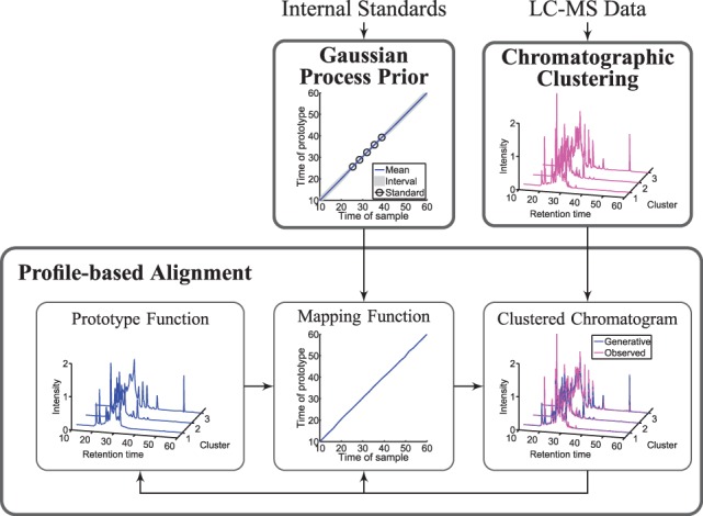
Three main components of the BAM: GP prior, chromatographic clustering and profile-based alignment

2.1 GP prior

For experiments in which an internal standard is added during the sample preparation, it is possible to identify a set of peaks with known identities and their RTs in each LC-MS run. With this information, adjustment can be made for each internal standard peak. This can be extended to other time points by conducting a GP regression to estimate the mapping function for each run with a regression function.

For each LC-MS run, we have the mapping relationship , where is the vector of original RTs for the R internal standard peaks, and is the corresponding assigned vector of reference times estimated by the average of each standard peak across multiple runs. A GP prior is defined over a latent mapping function of the observation , that is

(1)

where the mean function is an identity function, i.e. , and the covariance matrix is defined via a squared exponential covariance function κ, which reflects greater dependence between neighboring time points than distant points. The likelihood function is defined as 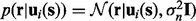. Based on the defined likelihood function and the GP, it can be shown (see Supplementary Material) that the predictive distribution of the mapping function at time t is a Gaussian with mean

(2)

and variance

(3)

where , and . This provides an effective way to infer the mapping functions, and the estimation depends on the number of standard peaks that can be reliably used and the coverage of RT by these peaks. As discussed in Section 1, we propose to use more comprehensive chromatographic information in our profile-based approach, in which the GP can be incorporated using the predictive distribution of the mapping function as the prior for subsequent estimation.

2.2 Profile-based alignment

In this section, we give a brief introduction of the previously reported profile-based alignment using a single chromatogram, e.g. base peak chromatogram from each LC-MS run (Tsai et al., 2013). Then, we discuss how we extend the model to handle multiple representative chromatograms simultaneously.

2.2.1 Single-profile modeling

We use a generative model to characterize the chromatographic elution process, where the observed chromatograms from N replicates, 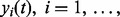, are assumed to share a similar profile characterized by the prototype function m(t). For the i-th chromatogram at RT t, the intensity value is referred to as the prototype function indexed by the mapping function , i.e. . By incorporating the variability of intensity using affine transformation, each chromatogram is modeled as

(4)

where a_i and c_i are scaling and translation parameters, and the errors ’ s are independent and identically distributed normal random variables 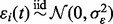. The prototype function is modeled with B-spline regression, , and the prior for each of the regression coefficients is defined as , where . The mapping function is a piecewise linear function characterized by a set of knots and their corresponding mapping indices . The prior of is specified by the GP prior as described in Section 2.1, and conjugate priors are chosen for the other model parameters.

2.2.2 Multi-profile modeling

For complex biological samples, collapsing the 3D data into a 2D chromatogram may blur originally distinct patterns. In such cases, the lack of a consistent pattern can hinder the estimation of mapping functions. To retain better chromatographic profiles, we propose to identify multiple representative chromatograms and perform the alignment by considering these chromatograms simultaneously. Extension of the generative model to handle multiple chromatograms can be made by introducing associated prototype functions of the representative chromatograms. That is,

(5)

where sample index , and chromatogram index . As in the single-profile (SP) modeling, the prototype function associated to each of the representative chromatograms is modeled with B-spline regression: , and the errors ’ s are independent and identically distributed normal random variables . The relationship between the G pairs of prototype functions and chromatograms is characterized by the mapping function.

2.2.3 Parameter inference

We use Markov chain Monte Carlo methods to draw inference based on the posterior distribution of model parameters. Once posterior estimates are obtained, the alignment can be performed based on the estimated mapping function, i.e. by replacing the RT t of the i-th run by . For parameters whose full conditionals have closed forms, we use Gibbs sampling to update their values. The only exception is , which is updated using an efficient block Metropolis–Hastings algorithm with a uniform proposal density that reflects the constraints on the boundaries. Details of the profile-based alignment including the full conditionals and the Metropolis–Hastings algorithm are provided in the Supplementary Material.

2.3 Chromatographic clustering

A critical issue involved in the multi-profile modeling is the identification of representative chromatograms from the LC-MS runs, where a trade-off between computational efficiency (less chromatograms) and information retention (more chromatograms) needs to be considered. Naïvely binning along the m/z dimension is not desirable, as chromatograms with similar m/z values do not necessarily resemble each other, and this would inevitably blur the chromatographic profiles. With an initial set of binned chromatograms at a resolution of 0.5 Da/bin, , we propose a clustering procedure consisting of screening of unqualified chromatograms, identification of exemplars and agglomerative clustering as follows.

2.3.1 Screening of unqualified chromatograms

Quality of each binned chromatogram is assessed by the mass chromatogram quality () and cross-correlation across LC-MS runs (), where the value of is computed using the component detection algorithm by Windig et al. (1996) to identify contaminated binned chromatograms in any of the LC-MS runs, and the cross-correlation is to gauge the consistency of the chromatographic pattern across the runs. The chromatograms are screened based on their quality. Only those satisfying the specified criterion, e.g. and , are retained for further processing.

2.3.2 Identification of exemplars

We apply the affinity propagation algorithm (Frey and Dueck, 2007) to identify exemplars of the retained chromatograms that best represent the whole chromatographic profiles, where Pearson correlation coefficient is used as the similarity measure, and the average of all the similarity measures is assigned as the exemplar preference. In affinity propagation, the sum of the similarity measure between each chromatogram and its exemplar is maximized, where the exemplar belongs to the chromatograms retained from the previous step.

2.3.3 Agglomerative clustering

Based on the set of identified exemplars, we perform the hierarchical agglomerative approach to cluster the exemplars, which is a bottom-up approach. Initially, each exemplar forms a singleton cluster, and two closest clusters are iteratively merged. At each level, the clustered chromatogram is summarized by

(6)

where denotes the set of chromatograms in the g-th cluster. The distance between two clusters is defined based on the overlapping level between two clustered chromatograms

(7)

Our goal is to cluster together chromatograms with less overlaps, i.e. agglomeration of fairly distinct chromatographic profiles, to better retain the chromatographic profiles. The procedure continues until all the exemplars are merged into a single cluster. Once the hierarchy is built, the number of clusters is determined using the L-method by Salvador and Chan (2004). On the plot of overlapping level against the number of clusters, we observe incremental decrease of the overlapping level and the L-method searches for the knee of the overlapping curve, where the benefit of adding an additional cluster starts decreasing. A sequence of two piecewise lines that fit the overlapping curve and their sum of squared errors are considered. The point minimizing the fitted sum of squared errors is chosen as the sufficient number of clusters.

3 LC-MS DATASETS

We applied BAM to three LC-MS datasets from metabolomic, proteomic and glycomic studies. These datasets present scenarios of real LC-MS experiments and capture the variabilities due to sample type, sample preparation methods and instrument condition, which all play a role in the quality of chromatographic reproducibility. It should be emphasized that none of these datasets can solely represent the complexity of all -omic studies. The metabolomic dataset is from a benchmark study by Lange et al. (2008), provided with ground-truth data (Available at http://msbi.ipb-halle.de/msbi/caap). The proteomic and glycomic datasets were generated by our group, where serum samples were spiked with internal standards, and peaks associated to the internal standards and the ground-truth data were determined. We provide the internal standards and the ground-truth data for both the proteomic and glycomic datasets in the Supplementary Material.

3.1 Metabolomic dataset

The metabolomic dataset consists of 24 LC-MS runs of Arabidopsis thaliana extract, acquired by an Agilent 1100 HPLC coupled to a Bruker micrOTOF-Q. To evaluate the alignment result, ground-truth data were generated based on ion annotation, correlation of chromatographic profile and consistency of peak. Comparison was carried out by evaluating recall and precision of the alignment results against the ground-truth data. For more details about this dataset, we refer interested readers to Lange et al. (2008).

3.2 Proteomic dataset

The proteomic experiment was designed to evaluate the application of the MARS Hu-14 column (Agilent Technologies) for depletion of high abundant proteins in human serum. The tryptic peptides are a mixture of the following five non-human proteins (Bruker-Michrom): Alcohol dehydrogenase (yeast), Carbonic anhydrase (bovine), Cytrochrome c (equine), Enolase (yeast) and Myoglobin (equine). Serum samples from five healthy individuals were analyzed. LC-MS/MS analysis of the serum samples was performed on an Agilent 1200 nano-LC coupled to a ThermoFisher LTQ-Orbitrap mass spectrometer, where data were acquired with double injections from two groups, with two different concentrations of the spike-in tryptic peptides. LC-MS/MS analysis of the internal standard mixture was also performed in duplicate right before the analysis of the serum samples. The mass spectrometer was scanned approximately every second using a 60 000 resolution setting. For each scan, up to five ions were automatically selected based on their intensities for the MS/MS analysis in the LTQ. The MS/MS spectra of the internal standard mixture were searched with Mascot, and 22 peaks corresponding to the internal standards were identified.

3.3 Glycomic dataset

The glycomic dataset is from an untargeted LC-MS study aimed at identifying N-glycan disease biomarkers. We analyzed human serum samples representing two distinct biological groups (cases and controls). The dataset was generated from sera of 11 cases and 12 controls. Sample preparation consists of release, purification, reduction and permethylation of N-glycans. Following sample preparation, LC-MS data were acquired using a Dionex 3000 Ultimate nano-LC system interfaced to an LTQ-Orbitrap Velos mass spectrometer on positive mode. An internal standard (galactose) was added to the serum samples before the LC-MS data acquisition, and five peaks (galactose 3–7) corresponding to the internal standard were consistently detected in all the analyzed samples.

4 RESULTS

We evaluate the alignment results based on the consensus list of the ground-truth data. Specifically, we compare the RT difference across LC-MS runs, the CV of extracted ion chromatograms and the peak-matching performance. The RT difference measures the difference between the largest and smallest RTs for a consensus peak. The CV evaluates the variability across chromatograms. The peak-matching performance is evaluated through precision and recall of the peak-matching results against the ground-truth data, as defined in Lange et al. (2008) and provided in the Supplementary Material. The SIMA model (Voss et al., 2011) is used for the peak-matching step. Internal standards are not included in the evaluation, as they are directly used in the alignment process. For confirmation purpose, we provide the alignment result in the Supplementary Material.

As there is no information about internal standards in the metabolomic dataset, the GP prior was not applied in this dataset, and only SP alignment was performed. The prior of the mapping function coefficients in this case is specified via a slope value 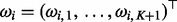, where is defined as , and it is assumed to follow a normal distribution with mean and variance truncated below by 0. Means (standard deviations) of the RT difference and CV values are compared based on the 1169 ground-truth peaks, where the RT values are in seconds. RT differences before and after alignment are 5.87 (3.16) and 3.86 (3.33), respectively, and CV values before and after alignment are 0.544 (0.120) and 0.474 (0.126), respectively. Although the RT alignment leads to a reduction of both RT difference and CV values, the peak-matching performance evaluated by (precision, recall) is barely improved, i.e. (0.826, 0.970) before alignment and (0.826, 0.971) after alignment. This is partly owing to the fact that RT variation is relatively small in this dataset. In addition, as the ground-truth data were generated based on ion annotation, further examination of the data is needed. More details and discussion are provided in the Supplementary Material.

Table 1 summarizes the results in the LC-MS proteomic and glycomic datasets, for the following procedures: no alignment performed to adjust the peak lists (raw), alignment performed using a GP regression as defined in Equation (2), SP alignment performed with no information about internal standards, SP alignment performed with a GP prior (GPSP) and multi-profile alignment performed (four chromatograms identified by the clustering procedure of Section 2.3) with a GP prior (GPMP). Each procedure was followed by a peak-matching step using SIMA. Most current LC-MS preprocessing pipelines do not adjust the peak lists detected upfront (raw) and directly apply a peak-matching procedure. SP alignment represents the current profile-based models including our earlier study (Tsai et al., 2013), where a single chromatogram is considered without using any information about internal standards. When chromatographic patterns are well captured by the base peak chromatogram, as in the proteomic dataset, the SP approach yields reasonable alignment result. Integration of internal standards (GPSP) and multiple chromatograms (GPMP) can lead to further improvement, as shown in Table 1. The improvement becomes significant in the glycomic dataset, which turns out to be the most challenging case. In the glycomic dataset, we observe that GP regression (with only five peaks of the internal standard) performs better than SP and comparably with GPSP. This is due to the lack of consistent pattern in the base peak chromatogram. Utilization of the internal standard and multiple chromatograms (GPMP) is advantageous as demonstrated by its consistently highest precision and recall, as well as its lowest RT and CV for both datasets. Figure 2 shows the measures of precision and recall of the five considered approaches, based on 72 pairs of tolerance parameters in SIMA. GPMP yields the best performance, with the least variability to the choice of parameters.

Table 1.

Performance comparison in the LC-MS proteomic and glycomic datasets

Performance measure	Proteomics					Glycomics
	Raw	GP	SP	GPSP	GPMP	Raw	GP	SP	GPSP	GPMP
RT	83.08 (20.84)	18.02 (22.74)	19.37 (28.56)	11.74 (19.61)	10.70 (20.67)	103.20 (32.63)	42.36 (29.76)	67.45 (42.39)	44.65 (31.35)	24.85 (27.21)
CV	1.634 (0.256)	1.118 (0.372)	1.150 (0.415)	1.060 (0.380)	1.052 (0.380)	1.194 (0.346)	0.931 (0.284)	1.090 (0.399)	0.978 (0.366)	0.821 (0.292)
Precision	0.937 (0.026)	0.983 (0.007)	0.985 (0.004)	0.988 (0.004)	0.990 (0.003)	0.943 (0.008)	0.965 (0.005)	0.967 (0.008)	0.976 (0.003)	0.980 (0.002)
Recall	0.638 (0.241)	0.933 (0.089)	0.952 (0.043)	0.962 (0.050)	0.970 (0.027)	0.612 (0.215)	0.819 (0.136)	0.773 (0.166)	0.829 (0.167)	0.907 (0.095)

Note: Five approaches are compared: no alignment performed (raw), alignment performed using a GP regression, SP alignment performed without using a GP prior (SP), SP alignment performed with a GP prior (GPSP) and multi-profile alignment (G = 4) performed with a GP prior (GPMP). Performance comparison based on RT difference (in seconds) across runs for consensus peaks, CV of the extracted ion chromatograms of consensus peaks, precision and recall. For RT difference and CV, means (standard deviations) are reported based on the 273 and 106 consensus peaks in the proteomic and glycomic datasets, respectively. For precision and recall, means (standard deviations) are reported based on 72 pairs of tolerance parameters of and RT in SIMA.

Fig. 2.

Measures of precision and recall in the (a) proteomic and (b) glycomic datasets, based on 72 pairs of tolerance parameters in SIMA. The five procedures compared are as follows: raw (asterisks), GP (circles), SP (squares), GPSP (triangles) and GPMP (diamonds)

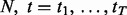
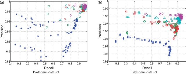
For the multi-profile alignment, representative chromatograms are first identified as discussed in Section 2.3. We use the L-method to determine the sufficient number of clusters as demonstrated in Figure 3. As shown in the figure, the sum of squared errors is minimized when the number of clusters is chosen as four in the glycomic dataset. For the four clustered chromatograms, the original and aligned chromatograms are shown in Figure 4. Similarly, for the proteomic data, the sufficient number of clusters to capture the chromatographic patterns was found to be four. Table 2 compares the peak-matching performance using multi-profile alignment for varying number of chromatographic bins or clusters. Chromatograms are derived either by binning along the m/z dimension or using the proposed chromatographic clustering procedure. As shown in the table, the chromatographic clustering procedure outperforms the binning approach. Incorporation of the GP prior shows significant improvement over those without the prior information, when using binning and when the number of chromatographic clusters is underestimated. This indicates that using the informative prior is beneficial for the profile-based alignment, especially when a consistent chromatographic pattern is unavailable. For a reasonable range of chromatographic clusters that capture the chromatographic patterns (), the results with or without integrating the internal standards are similar. We believe that further improvement can be achieved with the addition of more internal standards that allow better coverage of the RT.

Fig. 3.

Normalized overlapping level (a) and sum of squared errors (b) using the L-method in the glycomic dataset. The sufficient number of clusters is four

Fig. 4.

Clustered ion chromatograms in the glycomic dataset. (a–d) are the unaligned chromatograms and (e–h) are their corresponding aligned chromatograms. The inset is a zoomed part in the middle RT range of the chromatograms

Table 2.

Multi-profile alignment of the glycomic dataset with and without using a GP prior

Performance measure	Binning without GP prior				Clustering without GP prior				Binning with GP prior				Clustering with GP prior
	2	3	4	5	2	3	4	5	2	3	4	5	2	3	4	5
Precision	0.957	0.960	0.964	0.963	0.964	0.980	0.979	0.980	0.976	0.977	0.978	0.974	0.980	0.979	0.980	0.980
	(0.007)	(0.008)	(0.007)	(0.006)	(0.007)	(0.004)	(0.004)	(0.002)	(0.003)	(0.003)	(0.004)	(0.006)	(0.003)	(0.003)	(0.002)	(0.003)
Recall	0.766	0.783	0.770	0.780	0.796	0.906	0.910	0.913	0.848	0.856	0.830	0.837	0.904	0.904	0.907	0.908
	(0.138)	(0.122)	(0.147)	(0.154)	(0.138)	(0.094)	(0.099)	(0.092)	(0.151)	(0.141)	(0.160)	(0.156)	(0.098)	(0.099)	(0.095)	(0.096)

Note: Precision and recall are compared between cases where G chromatograms () are derived either by binning along m/z or using the chromatographic clustering procedure.

5 CONCLUSION

In this article, we propose a BAM for LC-MS data analysis. BAM improves on existing alignment methods by (i) using GP prior derived from internal standards and (ii) considering multi-profile modeling with representative chromatograms identified by a clustering approach. Application of the method to various LC-MS datasets shows that the proposed alignment approach greatly facilitates the subsequent peak-matching process by appropriate utilization of available information, which is often overlooked by current methods. Although this article focuses on using internal standards to derive the GP prior, it is also possible to specify the GP prior for the mapping relationship based on the identification of MS/MS spectra or targeted compounds.

The alignment model proposed here considers underlying patterns for LC-MS runs in samples drawn from the same biological group. When samples arise from different biological subgroups, the model needs to be extended to account for the heterogeneity across these subgroups. Future work will focus on developing a unified approach that allows the simultaneous alignment of samples from multiple biological groups to ensure coherence in the processing step and data comparability.

The LC-MS raw data, the preprocessed peak lists and the ground-truth data used in this article have all been made publicly available to serve as a benchmark for the evaluation of new preprocessing methods.

REFERENCES

- Aebersold R, Mann M. Mass spectrometry-based proteomics. Nature. 2003;422:198–207. doi: 10.1038/nature01511. [DOI] [PubMed] [Google Scholar]
- An HJ, et al. Glycomics and disease markers. Curr. Opin. Chem. Biol. 2009;13:601–607. doi: 10.1016/j.cbpa.2009.08.015. [DOI] [PMC free article] [PubMed] [Google Scholar]
- Christin C, et al. Time alignment algorithms based on selected mass traces for complex LC-MS data. J. Proteome Res. 2010;9:1483–1495. doi: 10.1021/pr9010124. [DOI] [PubMed] [Google Scholar]
- Fischer B, et al. Semi-supervised LC/MS alignment for differential proteomics. Bioinformatics. 2006;22:e132–e140. doi: 10.1093/bioinformatics/btl219. [DOI] [PubMed] [Google Scholar]
- Frenzel T, et al. A methodology for automated comparative analysis of metabolite profiling data. Eur. Food Res. Technol. 2003;216:335–342. [Google Scholar]
- Frey BJ, Dueck D. Clustering by passing messages between data points. Science. 2007;315:972–976. doi: 10.1126/science.1136800. [DOI] [PubMed] [Google Scholar]
- Hawkridge AM, Muddiman DC. Mass spectrometry-based biomarker discovery: toward a global proteome index of individuality. Annu. Rev. Anal. Chem. 2009;2:265–277. doi: 10.1146/annurev.anchem.1.031207.112942. [DOI] [PMC free article] [PubMed] [Google Scholar]
- Karpievitch Y, et al. Liquid chromatography mass spectrometry-based proteomics: biological and technological aspects. Ann. Appl. Stat. 2010;4:1797–1823. doi: 10.1214/10-AOAS341. [DOI] [PMC free article] [PubMed] [Google Scholar]
- Lange E, et al. A geometric approach for the alignment of liquid chromatography mass spectrometry data. Bioinformatics. 2007;23:i273–i281. doi: 10.1093/bioinformatics/btm209. [DOI] [PubMed] [Google Scholar]
- Lange E, et al. Critical assessment of alignment procedures for LC-MS proteomics and metabolomics measurements. BMC Bioinformatics. 2008;9:375. doi: 10.1186/1471-2105-9-375. [DOI] [PMC free article] [PubMed] [Google Scholar]
- Listgarten J, et al. Difference detection in LC-MS data for protein biomarker discovery. Bioinformatics. 2007;23:e198–e204. doi: 10.1093/bioinformatics/btl326. [DOI] [PubMed] [Google Scholar]
- Madsen R, et al. Chemometrics in metabolomics–a review in human disease diagnosis. Anal. Chim. Acta. 2010;659:23–33. doi: 10.1016/j.aca.2009.11.042. [DOI] [PubMed] [Google Scholar]
- Mann M, Kelleher NL. Precision proteomics: the case for high resolution and high mass accuracy. Proc. Natl Acad. Sci. USA. 2008;105:18132–18138. doi: 10.1073/pnas.0800788105. [DOI] [PMC free article] [PubMed] [Google Scholar]
- Patti GJ, et al. Innovation: metabolomics: the apogee of the omics trilogy. Nat. Rev. Mol. Cell Biol. 2012;13:263–269. doi: 10.1038/nrm3314. [DOI] [PMC free article] [PubMed] [Google Scholar]
- Rasmussen CE, Williams CKI. Gaussian Processes for Machine Learning. Cambridge, MA, USA: The MIT Press; 2006. [Google Scholar]
- Salvador S, Chan P. 16th IEEE International Conference on Tools with Artificial Intelligence. Boca Raton, FL, USA: 2004. Determining the number of clusters/segments in hierarchical clustering/segmentation algorithms; pp. 576–584. [Google Scholar]
- Smith CA, et al. XCMS: processing mass spectrometry data for metabolite profiling using nonlinear peak alignment, matching, and identification. Anal. Chem. 2006;78:779–787. doi: 10.1021/ac051437y. [DOI] [PubMed] [Google Scholar]
- Tomasi G, et al. Correlation optimized warping and dynamic time warping as preprocessing methods for chromatographic data. J. Chemom. 2004;18:231–241. [Google Scholar]
- Tsai T-H, et al. Profile-based LC-MS data alignment — a Bayesian approach. IEEE/ACM Trans. Comput. Biol. Bioinform. 2013;10:494–503. doi: 10.1109/TCBB.2013.25. [DOI] [PMC free article] [PubMed] [Google Scholar]
- Vandenbogaert M, et al. Alignment of LC-MS images, with applications to biomarker discovery and protein identification. Proteomics. 2008;8:650–672. doi: 10.1002/pmic.200700791. [DOI] [PubMed] [Google Scholar]
- Voss B, et al. SIMA: simultaneous multiple alignment of LC/MS peak lists. Bioinformatics. 2011;27:987–993. doi: 10.1093/bioinformatics/btr051. [DOI] [PubMed] [Google Scholar]
- Windig W, et al. A noise and background reduction method for component detection in liquid chromatography/mass spectrometry. Anal. Chem. 1996;68:3602–3606. [Google Scholar]
- Zaia J. Mass spectrometry and glycomics. OMICS. 2010;14:401–418. doi: 10.1089/omi.2009.0146. [DOI] [PMC free article] [PubMed] [Google Scholar]
Associated Data
This section collects any data citations, data availability statements, or supplementary materials included in this article.