Projection Reconstruction Magnetic Particle Imaging

Abstract

We acquire the first experimental 3-D tomographic images with magnetic particle imaging (MPI) using projection reconstruction methodology, which is similar to algorithms employed in X-ray computed tomography. The primary advantage of projection reconstruction methods is an order of magnitude increase in signal-to-noise ratio (SNR) due to averaging. We first derive the point spread function, resolution, number of projections required, and the SNR gain in projection reconstruction MPI. We then design and construct the first scanner capable of gathering the necessary data for nonaliased projection reconstruction and experimentally verify our mathematical predictions. We demonstrate that filtered backprojection in MPI is experimentally feasible and illustrate the SNR and resolution improvements with projection reconstruction. Finally, we show that MPI is capable of producing three dimensional imaging volumes in both phantoms and postmortem mice.

I. Introduction

Magnetic particle imaging (MPI) is an emerging medical imaging technique that directly detects ultra-small super-paramagnetic iron oxide particles (USPIOs) [1]–[3]. MPI has the potential to create in vivo maps of tracers with superior sensitivity, contrast, and safety compared to existing medical imaging modalities. Because MPI detects magnetic nanoparticles but not human tissue, it has contrast ideally suited to angiography, stem cell tracking, biomarker imaging, tracking of targeted chemotherapies, and functionalized USPIOs [4]–[6]. To date, MPI’s superior contrast and sensitivity have been demonstrated with phantom imaging experiments, as well as in mice injected intravascularly with USPIO tracers [7], [8].

In MPI, a time-varying magnetic field induces a nonlinear magnetization response in magnetic nanoparticles. This nonlinear response is localized using a magnetic field gradient and can be detected in an inductive receive coil. Initial imagers in MPI used a magnetic field free point (FFP) to localize USPIOs in the imaging volume. By rapidly scanning the FFP over a volume using electromagnets, a 3-D image of a USPIO concentration can be formed.

In contrast to a FFP, a field free line (FFL), which is a full line in space of zero magnetic field, localizes USPIOs along a line. Rapidly scanning this line in space creates a projection image of the particle concentration. By reducing image dimensionality from 3-D to 2-D, projection MPI improves speed by two orders of magnitude over imaging using a FFP. This speed improvement can be traded for signal-to-noise ratio (SNR) via averaging. In recent work, we demonstrated experimental images from a projection MPI scanner [9]. We described the x-space theory of an FFL, found the analytical point spread function of an x-space FFL scanner, and determined FFL homogeneity requirements.

A projection imaging format, coupled with sample or scanner rotation, can be used to acquire data necessary to reconstruct a 3-D image volume, as is done in computed tomography (CT). Fig. 1 illustrates the acquisition of a single projection, g(ℓ, θ), at a single rotation angle, θ. Multiple projections can be acquired by varying θ. Filtered backprojection (FBP), a projection reconstruction algorithm, is commonly used to reconstruct an image. As the name suggests, filtered backprojection first filters the projections using a ramp filter and subsequently projects (or smears) the filtered projections across the resulting image space at the angle of acquisition [10]. The multiple back-projected images are summed to reconstruct the output image. The step of adding multiple projections together increases SNR, a primary benefit of projection reconstruction. For the same acquisition time as a 3-D scan with a FFP, projection reconstruction MPI (PR MPI) has the potential to increase SNR by an order of magnitude due to signal averaging. This sensitivity gain would be useful to detect smaller concentrations of USPIO tracer.

Fig. 1.

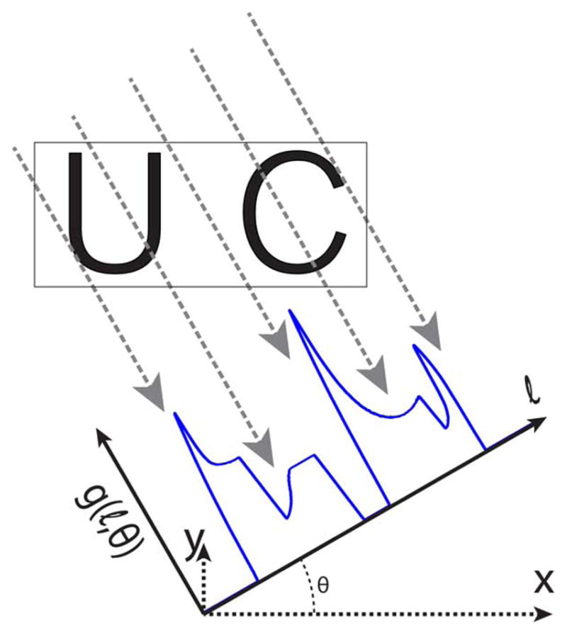
Diagram of projection reconstruction imaging. The FFL magnetic field is rotated at an angle θ followed by the acquisition of a single projection, g(l,θ). Multiple projections are acquired by varying θ, and a projection reconstruction algorithm is used to reconstruct a 3-D image. A single rotation angle of a projection reconstruction imaging sequence is shown. Here, a rotated projection is shown for clarity while sample rotation is used in our imaging system (see Fig. 2).

First introduced to the MPI field in 2008 [11], early FFL studies employed simulation and theory to demonstrate the SNR gain of projection reconstruction MPI. A simulation study introduced an electronically rotated and shifted FFL design, where a system matrix inversion with regularization was used to reconstruct images. This simulation showed SNR gains of the FFL over a traditional FFP acquisition [11]. Followup studies included designs to simplify and reduce power consumption of the initial FFL design and experimentally demostrated a shifted and rotated FFL [12]–[14]. An alternative FFL design with two Maxwell coil pairs has been introduced to reduce MPI system complexity [15]. Additionally, a study related projection reconstruction in MPI to the Fourier slice theorem and illustrated image reconstruction with two receive coils and an electronically rotated FFL [16].

However, to date, no experimental demonstration of projection reconstruction imaging has been done with an MPI system. FFL magnets have not yet been developed, built, and debugged with the capability of PR MPI. No studies have determined whether a FFL can be built with adequate homogeneity to image with PR MPI. The theoretical point spread function (PSF) for PR MPI has not been found. In addition, the SNR improvement of PR MPI with a FFL compared to 3-D imaging with a FFP has not been experimentally validated.

In this paper, we present the first experimental demonstration of PR MPI. We adapt x-space theory to projection reconstruction MPI, including the derivation of the theoretical PSF, resolution, SNR, and number of projections required. We augment our FFL projection MPI system with sample rotation to produce a projection reconstruction MPI system. Scanning methods using sample rotation, similar to this system, are common in MicroCT scanners [17], [18]. We then present projection reconstruction 3-D volumes of the PSF, imaging phantoms, and postmortem mice. This is the first experimental validation for projection reconstruction MPI techniques, which will enable higher SNR for detecting USPIO particles in vivo.

II. Theory

In this section, we describe the theory of projection reconstruction in x-space MPI. As seen in our PR MPI system in Fig. 2, we use the convention that the FFL is oriented along the y axis, the drive field excitation vector is along the z axis, and the slow focus or shift vector is along the x axis. We assume the particle response is instantaneous and has no relaxation effects.

Fig. 2.

Berkeley projection reconstruction MPI system. a) Diagram of the system magnets including a 2.4 T/m NdFeB gradient, and inductive shift, boost, transmit, and receive coils. b) System photograph additionally showing the sample holder, which includes a motor-driven rotary table that enables sample rotation.

To acquire multiple projection images necessary for projection reconstruction, we rotate the sample around the z axis, which is equivalent to FFL magnetic field rotation around the z axis for a system with excitation coils and receive coils oriented along the z axis. The instrument frame, [x y z]^T, is the nonrotated frame, while the sample frame, [x′ y′ z′]^T, is the rotated frame. The magnetic field of the FFL oriented along the y axis can be described using a gradient matrix H(x) = Gx. This field is translated along the x axis using a homogeneous focus or shift field, H_s = H_xî. The particles are excited along the z axis by a homogeneous field, H_e = H_zk̂, as illustrated in Fig. 3. The combined magnetic field becomes

Fig. 3.

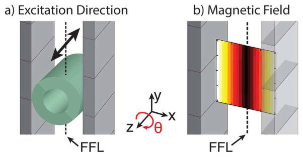
FFL excitation diagram and magnetic field plot. a) Diagram of the permanent magnets that generate the FFL and of the solenoidal transmit coil that excites USPIOs at 20 kHz. The arrow above the transmit coil indicates that the excitation direction is along the z axis. The ~2 Hz slow shift of the FFL occurs along the x axis. b) Magnetic field plot of the FFL with darker colors corresponding to smaller field strengths.

$$\begin{array}{l}\mathbf{H}(\mathbf{x})=\mathbf{Gx}+H_x\widehat{\mathbf{i}}+H_z\widehat{\mathbf{k}}\\ =\left[\begin{array}{ccc}{G}_{xx}& 0& 0\\ 0& 0& 0\\ 0& 0& G_{zz}\end{array}\right]\left[\begin{array}{c}x\\ y\\ z\end{array}\right]+\left[\begin{array}{c}{H}_x\\ 0\\ H_z\end{array}\right]\end{array}$$ (1)

where x [m] is the position vector in the instrument coordinate system and μ₀G_ab [T/m] is the partial derivative of the magnetic field in the a direction with respect to b [9], [16]. μ₀G_ab is also known as the gradient strength of the system. μ₀ = 4π × 10⁻⁷ T · m/A is the permeability of free space. G_xx = −G_zz as required by Maxwell’s equations.

In Appendix A, we derive the magnetic field of the shifted and rotated FFL. To determine where the FFL lies in space, we calculate the magnitude of the magnetic field (which is squared to simplify the result here)

$${\mid {\mathbf{H}}^{\prime }({\mathbf{x}}^{\prime },\theta )\mid }^2={(G_{zz}{z}^{\prime }+H_z)}^2+G_{zz}^2{(x^{\prime }cos\theta +y^{\prime }sin\theta -H_x/G_{zz})}^2$$ (2)

where θ [rad] is the angle of rotation. By inspection, we see that the field is zero when

$$z^{\prime }=-H_z/G_{zz}$$ (3)

and

$$x^{\prime }cos\theta +y^{\prime }sin\theta =H_x/G_{zz}.$$ (4)

We define

$$\ell =H_x/G_{zz}.$$ (5)

Thus, the FFL lies on

$$x^{\prime }cos\theta +y^{\prime }sin\theta =\ell$$ (6)

at a z position defined by the H_z excitation field and the gradient. Note that physically ℓ [m] represents the shift position perpendicular to the FFL. This is the standard notation used in CT [10]. The USPIO signal is integrated along this line, allowing a projection image of the sample to be acquired at any rotation angle as illustrated in Fig. 1. The variables H_x, H_z, and θ give us precisely the control we require to collect a complete set of projection data.

After acquiring projections, a 3-D volume can be created using PR methods such as the direct Fourier method, convolution backprojection, FBP, or other statistical, iterative, and optimization approaches [10], [19]–[22]. In this work, we used filtered backprojection due to its simplicity and robustness. The FBP algorithm first filters the acquired projections with a ramp filter in the spatial frequency domain and then backprojects the filtered projections. This operation essentially smears the filtered projections across the reconstructed image at the angle of incidence. The backprojected images are added to create a 3-D volumetric image.

To derive the PSF for projection reconstruction MPI, we can start from the PSF for a single projection, h(x) [9]. The PSF after PR can then be calculated using the inverse Abel transform [23], which is equivalent to the Fourier transform followed by the inverse Hankel transform

$$h_{\text{PR}}(r)={\mathcal{A}}^{-1}\{h\}={\mathcal{H}}^{-1}\{\mathcal{F}\{h\}\}$$ (7)

where is the inverse Abel transform operator, is the inverse Hankel transform operator, and is the forward Fourier transform operator. There is no closed-form expression for the Fourier transform of the MPI PSF along the x axis, but fortunately, it is well approximated [<1% rms full-scale error as calculated by (17)] by a Lorentzian. The result is a closed form approximation of the PR PSF in the xy plane

$${\widehat{h}}_{\text{PR}}(r)=\sum _{k=1}^2{\beta }_k{\left({\alpha }_k^2+r^2\right)}^{\frac{-3}{2}}$$ (8)

where r [m] is the distance along the radial axis. α₁, α₂, β₁, and β₂ are fitted constants determined in Appendix B. Equation (8) is accurate within a 2.4% rms full scale error [calculated with (17)] when compared across a 6 cm FOV to the theoretical PSF, which can be computed via filtered backprojection on the 1-D projection PSF. This approximation allows us to determine how system and particle parameters affect resolution and the number of projections required in PR MPI. A detailed derivation of this approximation is included in Appendix B.

We use the approximate PSF in (8) to determine the resolution of a PR MPI system. The resolution according to the Houston criterion [24], or full-width at half-maximum (FWHM), of (8) is

$${\text{FWHM}}_{\text{PR}}\approx \frac{34k_{b}T}{{\mu }_0{G}_{xx}\pi M_{\text{sat}}{d}^3}$$ (9)

where μ₀M_sat ~ 0.6 T is the saturation magnetization, d[m] is the particle diameter, k_b = 1.38 × 10⁻²³ m² · T · A · K⁻¹ is Boltzmann’s constant, and T [K] is the temperature. Note that the FWHM resolution before PR also has the same form; however, PR imaging improves resolution by approximately 40% along the x axis. The resolution scales inversely with the gradient and the cube of the particle diameter. In a system with a 2.4 T/m gradient and with particles that can be modeled as theoretical particles of 22.7 nm in diameter (see Section III-C), we would expect a FWHM of 3.3 mm in the xy plane.

We also use the PSF of (8) to determine the minimum number of evenly-spaced projections between 0° and 180° required to avoid aliasing in a PR image. As discussed in Appendix C, we can use the following formula as guidance [19]:

$$N_{\text{proj}}>\pi ·{\text{FOV}}_{xy}·K_{max}$$ (10)

where FOV_xy [m] is the maximum field-of-view (FOV) of x and y and is set by the system user. K_max[m⁻¹] is the largest spatial frequency in the system, which is determined from the system point spread function (PSF). In a system with a 2.4 T/m gradient and with particles modeled as 22.7 nm in diameter (see Section III-C), K_max ≈ 1/(2 FWHM) = 0.15 mm⁻¹. With a FOV_xy = 6 cm, 28 projections are necessary to avoid aliasing.

The number of projections acquired also affects SNR of the resulting image. In general, SNR increases by the square root of the number of averages acquired in a system, assuming that the noise is independent and identically distributed. In projection reconstruction, this means that SNR improves $\propto \sqrt{N}$, where N is the number of projections acquired. In practice, if we increase the number of projections from 25 to 100, we will double our SNR as well as decrease aliasing artifacts.

III. Methods

A. Imaging System Construction

A diagram and photograph of our imaging system are shown in Fig. 2. This system is described in more detail in [9]. We used two NdFeB permanent magnet sections to produce the FFL. Each section was created with six NdFeB permanent magnets assembled with matching magnetization orientation. The two sections were then assembled with opposing magnetization orientation to produce a FFL. This configuration produced a μ₀G_zz = −μ₀G_xx = 2.4 T/m magnetic field gradient along both the x and z axes with the FFL oriented along the y axis.

We attached two electromagnets (GMW 11901111, San Carlos, CA) to shift the FFL in the x direction and two custom electromagnets to shift the FFL in the z direction. Switching amplifiers (Copley Controls 234) drove these coils with a maximum 350 A peak current, which produced a x direction FOV of 6 cm. A linear amplifier (AE Techron LVC5050) drove a resonant transmit coil, which created the 20 kHz drive field oriented in the z direction. The receive chain consisted of an inductive receive coil, a notch filter at the fundamental drive frequency, and low noise preamplifiers (SR560 and SIM911). Custom software (Mathworks Matlab, Natick, MA) controlled a data acquisition card (NI PCIe-6363, Austin, TX), which drove the amplifiers and digitized the signal. A one axis translation stage (Velmex, Bloomfield, NY) was used to increase the FOV to a maximum of 22 cm in the z direction using a moving table scan.

B. Image Acquisition and Projection Reconstruction

To obtain an MPI tomographic 3-D volume, we employed FBP after acquiring projection images at multiple angles. A motor driven rotary table (Velmex, Bloomfield, NY) rotated the sample to allow the acquisition of images at linearly spaced angles from 0° to 180°. Procedurally, the scanner obtained a projection image at one rotation angle, rotated the sample, and then acquired another projection image [see Fig. 6(c)]. After acquiring all images, the FBP algorithm was employed. The algorithm selected a 1-D slice parallel to the x axis in each image at corresponding z locations and then filtered each slice using a ramp filter in the spatial frequency domain to compensate for denser sampling at the center of [10], [20]. After filtering, the slices were backprojected at the acquisition angle, and a 3-D volume was reconstructed. Projection scans were taken twice, once in the forward translation z direction and once in the reverse direction, and were averaged to form the final image.

Fig. 6.

Undeconvolved filtered backprojection MPI experimental images. a) Acrylic phantoms stacked in preparation for imaging. b) Photographs of phantoms with 50 mM Resovist (10× diluted). c) Four of 180 acquired projection images with rotation angle, θ, denoted on each image. d) Maximum intensity projection of the 3-D volume reconstructed using filtered backprojection on the 180 projection images. e) Two slices of the 3-D imaging volume at the plane of each imaging phantom with slice thickness of 0.5 mm. Each projection image acquisition took 39 s for a total imaging time of 117 min with N = 2 averages (N = 1, 59 min) with a 6 cm×12 cm FOV.

After reconstructing a 3-D image volume, the software exported the entire volume in DICOM file format. The DICOM files were imported to Osirix (Pixmeo, Switzerland), where maximum intensity projection and volume rendered images were created.

C. PSF Measurement and Comparison

To measure the PSF of our imaging system, we imaged a 3.5-μL vial of undiluted 0.5 M Resovist (Schering AG, Germany), a USPIO tracer for MRI. The Resovist vial contained the sample within 3 mm³, which was smaller than the resolution of our imaging system and could be considered a point source. The scanner acquired 180 projection images, each with an acquisition time of 16 s and a FOV of 6 cm×5.6 cm. A 3-D volume was then reconstructed as described in Section III-B.

Projection PSF calculations were performed using (14) and approximate PR PSFs were calculated using (8). For theoretical PR PSFs, we used (14) and applied filtered backprojection. Parameters were chosen to match our imaging system: μ₀G_zz = −μ₀G_xx = 2.4 T/m and T = 300 K. The particle diameter of Resovist has been reported as many different diameters [9], [25]. To determine the effective Resovist diameter in our sample, we fitted the theoretical projection PSF of (14) to the measured projection PSF with the particle diameter as the free parameter. This fit resulted in a diameter d = 22.7 nm. This diameter was used for all calculations. Since the dc information is not available in MPI data [26]–[28], we restored the dc value by assuming the MPI signal at the boundaries of the image was zero.

D. Phantom Experiments

To test the performance of our projection reconstruction MPI system, we created custom acrylic phantoms with Resovist tracer. The phantoms were composed of three laser cut sheets of acrylic with the middle layer containing the desired Resovist distribution pattern. Fig. 6(a) shows images of two acrylic phantoms stacked to create a 3-D Resovist distribution. Phantom imaging was performed with 180 projection images, a 6 cm×12 cm FOV, and an acquisition time of 39 s per projection. The total acquisition time was 2 h. Filtered backprojection was used to create a 3-D volume as described in Section III-B.

A helical imaging phantom [pictured in Fig. 7(a)] was created using cylindrical piece of acrylic with a 3.4 cm outer diameter. Tubing with ID 0.8 mm (OD 1.4) was wrapped around the acrylic and was filled with 50 mM Resovist (10×diluted). Sixty projections, each with a 6 cm×12 cm FOV and 39 s scan time were taken. The entire volume was acquired in 39 min.

Fig. 7.

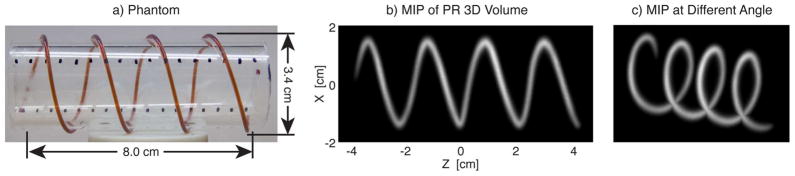
Phantom imaging. a) Photograph of a helical imaging phantom. Tubing with ID 0.8 mm (OD 1.4 mm) was filled with 50 mM Resovist (10× diluted). b) Maximum intensity projection (MIP) image with no deconvolution taken in our projection reconstruction MPI scanner. c) MIP at a different angle to illustrate the 3-D volume. A total of 60 projection images were acquired with a time of 39 s each and a 6 cm×12 cm FOV. The total imaging time was 39 min.

E. Mouse Imaging

We prepared a mouse for imaging by injecting 100 μL of undiluted Resovist into the tail vein and sacrificing after 30 s. The mouse was then imaged in the PR MPI system with 180 projections, each with a FOV of 6 cm×12 cm along the x and z axes, respectively. Each projection image took 3 min to acquire for a total imaging time of 540 min. After acquisition and reconstruction using FBP, we applied deconvolution with Wiener filtering [29] using the theoretical PSF. The small amount of deconvolution sharpens the image by reducing the effect of the long tails of the PSF.

IV. Results

In Fig. 4, we compare the theoretical PSF with a PSF measured from our imaging system. Images in the left column show the xz plane while images in the right column show the xy plane. The top set of four boxed images compares projection format PSFs while the bottom set compares projection reconstruction format PSFs. Note the close agreement between theoretical and measured PSFs.

Fig. 4.

Projection PSF and projection reconstruction PSFs using filtered back-projection. Cross section along the red lines are shown in Fig. 5. (row a) Diagram indicating the orientation of the plots in the same column below. (row b) Theoretical PSF using (14). (row c) Measured projection PSF. (row d) Theoretical projection reconstruction PSF obtained using filtered backprojection on row b. (row e) Measured projection reconstruction PSF. Acquisition time for each projection image was 16 s per image, the XZ FOV was 6 cm × 5.6 cm and 180 projections were acquired.

Fig. 5 compares image cross sections of measured, theoretical, and approximate PSFs in both projection and projection reconstruction formats. Fig. 5(a) plots a cross section of the measured and theoretical projection PSFs in Fig. 4(b) and (c), demonstrating agreement between the two. Fig. 5(b) plots cross sections from the measured and theoretical projection reconstruction PSF from Fig. 4(d) and (e). Fig. 5(b) also plots an approximate projection reconstruction PSF, calculated from (8). For comparison, the FWHM is listed for each plot. Note the slight decrease in FWHM in the PR results over the projection results as predicted in Section II. Also note the close match in theoretical, approximate, and measured plots and FWHM values.

Fig. 5.

Projection PSF and projection reconstruction PSF cross sections from Fig. 4. a) Measured and theoretical projection PSFs. Theoretical PSF calculated using (14). b) Measured, theoretical, and approximate Projection Reconstruction PSFs. The approximate PSF was obtained using (8), while the theoretical PSF was obtained via filtered backprojection on (14).

Fig. 6(c) shows four of the 180 projections acquired at multiple angles of rotation around the theta axis for our stacked acrylic imaging phantom. A maximum intensity projection through the imaging volume is displayed in Fig. 6(d). Fig. 6(e) shows two slices through the image volume. No deconvolution has been performed in any of the images in Fig. 6. Note, we can see two large air bubbles in both the photograph of the phantom and the output PR image. This can also be seen but with more difficulty in the projection images. Also, in the projection images of Fig. 6(c), note the signal summation that occurs along the field free line, which causes bright points at differing locations along the phantom image depending on rotation angle. These bright points occur at locations where the FFL integrates signal in both acrylic phantoms. While we see these bright spots in the projection images, the PR images fully resolve all features in 3-D. The ability to resolve the bubble and the lack of signal summation illustrate the diagnostic quality improvement of 3-D PR imaging over projection format imaging.

Fig. 7 contains maximum intensity projection images from a helical phantom. Two perspectives are shown of the reconstructed volume. Once again, these images illustrate the capability for very high SNR with PR MPI.

Fig. 8 shows a projection reconstruction image of a postmortem mouse injected with Resovist. The tracer accumulation can be seen in the heart, liver, and brain.

Fig. 8.

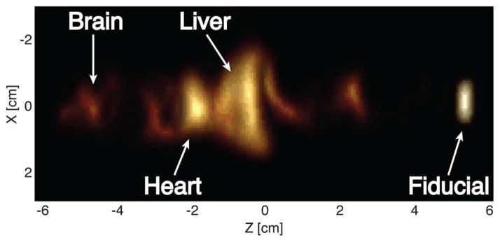
PR MPI image of a mouse injected with 100 μL of 0.5 M Resovist into the tail vein and sacrificed after 30 s. The tracer accumulation appears in the heart, liver, and brain. 180 projection images were taken, each with a 6 cm×12 cm FOV and 3 min acquisition time.

V. Discussion

Here, we have demonstrated the first experimental implementation of filtered back projection 3-D MPI scanning. The same projection reconstruction MPI scanner could be used in a 2-D projection format to produce real-time images or with averaging to produce high SNR 2-D images. The flexibility enabled by FFL imaging for high speed or high SNR 2-D imaging, as well as high SNR 3-D images, could be extremely useful in the clinic. This relationship could be similar to the relationship that currently exists between X-ray and CT. Applications such as angiography demand a high speed format to faithfully capture the range of cardiac motion so X-ray fluoroscopy is often used. Patients would benefit from projection MPI that utilizes no ionizing radiation and tracers that are completely safe, especially for CKD patients [30]. For applications not requiring high speed but benefitting from a high SNR 3-D image, CT is used. In MPI, possible applications of this format include cancer and stem cell imaging.

This paper presents the first experimental proof that the homogeneity of a real-world, inexpensive permanent magnet FFL can be made adequately uniform (with minimal fading [9]) to produce artifact-free FBP reconstructions. This bodes well for future higher strength FFL magnets. In the future, we intend to develop a scaled-up PR MPI system. Such a system could include a 20 T/m superconducting gradient with a 256³ image grid. A gradient of this strength would have a 400 μm xy plane resolution with Resovist according to (9). With a 6 cm FOV, we would need to acquire 235 projections to avoid aliasing according to (10). With MPI we have the benefit that additional projections do not cause additional patient radiation dose since no ionizing radiation is involved. Challenges to development of such a system would include higher receiver bandwidth, better FFL magnet homogeneity (to prevent fading artifacts [9]), and reconstruction time scale-up.

We also plan to implement a helical moving-bed scan similar to current CT technology. We estimate that we could acquire a full 3-D volume in approximately 5 min with our current imaging system via this scanning pattern (partial FOV of 8 mm, helical pitch of 4 mm to allow 50% overlap, 10 s per rotation). Alternatively, we could implement z axis focus field coils (currently unused in this work), which would allow 3-D volume acquisition in approximately 30 s (partial FOV of 8 mm, z axis shift of 4 cm and helical pitch of 4 cm, 10 s per rotation). Future scanner hardware development could also include other rotation methods such as gantry rotation or electronic FFL rotation.

As an alternative to Nyquist sampling, we could use compressed sensing techniques to reduce the number of projections taken and speed imaging time. In a human sized scanner with a bore of 30 cm and a gradient of 8 T/m (1 mm resolution with Resovist), 470 projections would be required for nonaliased sampling using the Nyquist criteria. Compressed sensing could allow a much smaller number of projections, thus allowing a faster image acquisition for time resolved datasets [31]–[33].

It is interesting to compare MPI projection imaging to MRI projection imaging. With MPI, there is absolutely no concern with phase decoherence along the projection line because all the SPIOs are locked in synchrony with the excitation field. This is in sharp contrast to projection MRI, where B0 inhomogeneity is typically inadequate to prevent excessive decoherence, which is called T2* dephasing in MRI.

The approximate and measured PSFs of Fig. 5 match well, illustrating the accuracy of the approximation. The improvement in FWHM after FBP occurs due to image sharpening from the ramp filter. The resolution (and SNR) benefit of PR MPI could be used to view smaller arteries in a high resolution 3-D PR MPI as opposed to 3-D scan with a FFP.

Equation (10) suggests that we only need 28 instead of 180 projections to obtain a nonaliased PR MPI image with our system. Here, we have used more projections to demonstrate artifact free and high SNR images. SNR is extremely high even in our university prototype. This bodes well for the future sensitivity of a professionally engineered system.

VI. Conclusion

In this work, we presented the world’s first experimental projection reconstruction MPI system. A permanent magnet FFL was shown to be buildable to the tolerance required for artifact-free FBP. We designed, built, and debugged the associated PR MPI subsystems such as the drive field generation, focus field generation, receive channels, sample rotation, and image acquisition. The approximate PR PSF was derived and shown to correspond accurately to data. The theoretical FWHM, number of projections required, and the SNR gain in projection reconstruction MPI were derived as well. We demonstrated that FBP in MPI is experimentally feasible and illustrated the SNR and resolution improvement with PR. We then demonstrated that MPI is capable of producing three dimensional imaging volumes in both phantoms and postmortem mice. This is promising for the future of PR MPI.

Appendix A. FFL Rotation

An FFL magnetic field can be described using a gradient matrix in the instrument frame as

$$\begin{array}{l}\mathbf{H}(\mathbf{x})=\mathbf{Gx}\\ =\left[\begin{array}{ccc}-\alpha G_{zz}& G_{xy}& G_{xz}\\ G_{xy}& (\alpha -1)G_{zz}& G_{yz}\\ G_{xz}& G_{yz}& G_{zz}\end{array}\right]\left[\begin{array}{c}x\\ y\\ z\end{array}\right]\end{array}$$

where x is the position vector and G_ab is the partial derivative of the magnetic field in the a direction with respect to b. We design the FFL magnet such that α = 1 (so the FFL lies along the y axis) and the cross terms G_xy, G_xz, and G_yz are zero so that the field becomes

$$\mathbf{H}(\mathbf{x})=\mathbf{Gx}=\left[\begin{array}{ccc}-G_{zz}& 0& 0\\ 0& 0& 0\\ 0& 0& G_{zz}\end{array}\right]\left[\begin{array}{c}x\\ y\\ z\end{array}\right].$$ (11)

We then rotate the coordinate system about the z axis using the rotation matrix

$${\mathbf{R}}_{\mathbf{z}}(\theta )=\left[\begin{array}{ccc}cos\theta & -sin\theta & 0\\ sin\theta & cos\theta & 0\\ 0& 0& 1\end{array}\right]$$ (12)

where θ is the angle of rotation. The coordinate system after rotation is x′ = R_zx, and the field after rotation is H′ = R_zH. R_z is an orthogonal matrix so ${\mathbf{R}}_z^{-1}={\mathbf{R}}_z^T$. The field is translated along the x axis in the instrument coordinate system by a homogeneous field, H_s = H_xî. The particles are excited along the z axis by a homogeneous field, H_e = H_zk̂. The field in the sample’s rotated coordinate system becomes

$${\mathbf{H}}^{\prime }({\mathbf{x}}^{\prime },\mathit{\theta })={\mathbf{R}}_{\mathbf{z}}\left(\mathbf{G}{\mathbf{R}}_{\mathbf{z}}^{\mathbf{T}}{\mathbf{x}}^{\prime }+H_x\widehat{\mathbf{i}}+H_z\widehat{\mathbf{k}}\right).$$

The x′, y′, and z′ axes are in the rotated (sample) coordinate system and correspond to the x, y, and z axes, respectively, in the instrument coordinate system. Note that in the sample’s coordinate system, sample rotation and FFL rotation are equivalent operations. The trace of H′ remains zero as required by Maxwell’s equations. After simplification, each component of the magnetic field is then

$${\mathbf{H}}^{\prime }({\mathbf{x}}^{\prime },\mathit{\theta })=\left[\begin{array}{c}-G_{zz}cos\theta (x^{\prime }cos\theta +y^{\prime }sin\theta -H_x/G_{zz})\\ -G_{zz}sin\theta (x^{\prime }cos\theta +y^{\prime }sin\theta -H_x/G_{zz})\\ G_{zz}{z}^{\prime }+H_z\end{array}\right].$$

To determine where the field free line lies in space, we take the magnitude squared of the magnetic field

$${\mid {\mathbf{H}}^{\prime }({\mathbf{x}}^{\prime },\mathit{\theta })\mid }^2={(G_{zz}{z}^{\prime }+H_z)}^2+G_{zz}^2{(x^{\prime }cos\theta +y^{\prime }sin\theta -H_x/G_{zz})}^2.$$ (13)

By inspection, we see that the field is zero at

$$z^{\prime }=-H_z/G_{zz}$$

and

$$x^{\prime }cos\theta +y^{\prime }sin\theta =H_x/G_{zz}.$$

We define

$$\ell =H_x/G_{zz}.$$

Thus, the FFL lies on

$$x^{\prime }cos\theta +y^{\prime }sin\theta =\ell$$

where ℓ[m] is the shift position perpendicular to the FFL. This is the standard notation used in CT [10].

Appendix B. PSF Derivation

We calculate the 2-D PSF based on the normal component of the collinear FFL PSF [3]. The collinear PSF is used because the transmit excitation vector and maximum receive sensitivity are aligned (along the z axis). The normal component refers to the fact that the image axis, the x axis, is perpendicular to the transmit axis, the z axis. We begin with the expression for the multidimensional PSF

$$\mathbf{h}(\mathbf{x})=\stackrel{.}{\mathcal{L}}[\Vert \mathbf{Gx}\Vert /H_{\text{sat}}]\frac{\mathbf{Gx}}{\Vert \mathbf{Gx}\Vert }{\left(\frac{\mathbf{Gx}}{\Vert \mathbf{Gx}\Vert }\right)}^T\mathbf{G}+\frac{\mathcal{L}[\Vert \mathbf{Gx}\Vert /H_{\text{sat}}]}{\Vert \mathbf{Gx}\Vert /H_{\text{sat}}}\left(\mathbf{I}-\frac{\mathbf{Gx}}{\Vert \mathbf{Gx}\Vert }{\left(\frac{\mathbf{Gx}}{\Vert \mathbf{Gx}\Vert }\right)}^T\right)\mathbf{G}.$$ (14)

We then set the excitation vector along the z axis, set θ = 0 so the gradient matrix is G = diag(G_xx, 0, G_zz), and calculate the PSF along the x axis

$$h_{\Vert }(x,0,0)=\frac{\mathcal{L}[\mid G_{xx}x\mid /H_{\text{sat}}]}{\mid G_{xx}x\mid /H_{\text{sat}}}{G}_{zz}$$

where we use the || symbol to denote that we are using the collinear portion of the PSF.

Substituting the Langevin function, we get the following expression for the collinear 1-D PSF along the x axis [3]:

$$h_{\Vert }(x,0,0)=\left(\frac{coth(G_{xx}x/H_{\text{sat}})}{G_{xx}x/H_{\text{sat}}}-\frac{H_{\text{sat}}^2}{{(G_{xx}x)}^2}\right)G_{zz}$$ (15)

where the unnecessary absolute values have been removed.

To determine the two dimensional PSF after projection reconstruction, we take the inverse Abel transform of the 1-D PSF which is the mathematical operation for filtered backprojection [23]. This is equivalent to taking the Fourier transform and subsequently applying the inverse Hankel transform

$$h_{\text{PR}}(r)={\mathcal{A}}^{-1}\{h_{\Vert }(x,0,0)\}={\mathcal{H}}^{-1}\{\mathcal{F}\{h_{\Vert }(x,0,0)\}\}.$$

The function for h_|| does not have a simple Fourier transform so we approximate the function with two Lorentzian functions

$${\widehat{h}}_{\Vert }(x,0,0)=\sum _{k=1}^{2}2{\beta }_k\frac{1}{x^2+{\alpha }_k^2}$$ (16)

where α₁ = 3.6H_sat/G_xx, α₂ = 27.8H_sat/G_xx, ${\beta }_1=0.8{\alpha }_1^2{G}_{zz}/6$, and ${\beta }_2=0.2{\alpha }_2^2{G}_{zz}/6$. H_sat = k_bT/(μ₀m) [A/m] is the field required for saturation, and m = M_satπd³/6 [T/m³] is the magnetic moment. Parameters α_k are related to the width of the function while β_k determine the weighting of the two components. We chose the function’s form from the closest match from Fourier transform tables and chose parameters α_k and β_k by fitting (16) to (15). Equation (16) is accurate to one percent rms error as a percentage of full scale when measured within a FOV greater than or equal to 6 cm. The rms full scale error is defined as

$${\text{error}}_n=\frac{(a_n-b_n)}{max(a)}$$ (17)

where a_n and b_n are the values compared at each index, n. We then calculate the root mean squared value from the error vector. The projection PSF, its approximation, and the rms full scale error are illustrated in Fig. 9.

Fig. 9.

Projection point spread function from (15) and a two lorentzian approximation from (16) as well as the error as a percentage of full scale calculated with (17).

Using the 1-D Fourier transform pair

$$\frac{2b}{b^2+x^2}\stackrel{\mathcal{F}}{\to }2\pi e^{-b\mid 2\pi q\mid }$$

the above approximation for ĥ_|| has a Fourier transform

$${\widehat{H}}_{\Vert }(q)=\sum _{k=1}^2\frac{{\beta }_k}{{\alpha }_k}2\pi e^{-{\alpha }_{k}2\pi q}.$$

Next, we calculate the inverse Hankel transform, which is defined from 0 to ∞; thus we drop the absolute value and use the transform pair

$$b^{-1}2\pi e^{-b2\pi q}\stackrel{{\mathcal{H}}^{-1}}{\to }{(b^2+r^2)}^{-\frac{3}{2}}.$$

We arrive at the analytical approximation for the projection reconstruction PSF

$${\widehat{h}}_{\text{PR}}(r)=\sum _{k=1}^2{\beta }_k{({\alpha }_k^2+r^2)}^{-\frac{3}{2}}.$$ (18)

Appendix C. Number of Projections

A minimum number of projections are required to avoid spatial aliasing in a projection reconstruction image. Aliasing in a PR system typically manifests as streaking artifacts. The artifacts can reduce the effective resolution of the image as well as impact the perspicuity of the images. To avoid streaking artifacts and a loss of effective resolution we can choose a sample rate that meets the Nyquist criterion. We choose system parameters such that

$$\mathrm{\Delta }k\le \frac{1}{{\text{FOV}}_{xy}}$$

where Δk is the spatial frequency and FOV_xy is the maximum FOV in the x axis and y axis. Δk is controlled by the number of projections and how finely the projections are sampled in k-space, as illustrated in Fig. 10.

Fig. 10.

The worst case distance between samples in projection reconstruction occurs at the outer radius of successive rotated projections. From these samples, we determine the maximum angular difference between projections and the minimum number of projections required to avoid aliasing according to the Nyquist criterion for projection reconstruction.

The worst-case sampling separation in k-space is

$$\mathrm{\Delta }k=2K_{max}sin\left(\frac{\mathrm{\Delta }\theta }{2}\right)$$

where K_max is the radius covered in k-space and Δθ is the angular sampling increment. Using a small angle approximation, we derive the following formula as guidance:

$$\mathrm{\Delta }\theta <\frac{1}{FO{V}_{xy}·K_{max}}.$$

Substituting

$$N_{\text{proj}}=\frac{\pi }{\mathrm{\Delta }\theta }$$

where N_proj is the number of projections, we arrive at the formula for the number of projections needed to avoid aliasing

$$N_{\text{proj}}>\pi ·FO{V}_{xy}·K_{max}.$$

This is consistent with the result reported in Bracewell and Riddle [19].

References

- 1.Gleich B, Weizenecker J. Tomographic imaging using the nonlinear response of magnetic particles. Nature. 2005 Jun;435(7046):1214–1217. doi: 10.1038/nature03808. [DOI] [PubMed] [Google Scholar]
- 2.Goodwill PW, Conolly SM. The x-space formulation of the magnetic particle imaging process: 1-D signal, resolution, bandwidth, SNR, SAR, and magnetostimulation. IEEE Trans Med Imag. 2010 Nov;29(11):1851–1859. doi: 10.1109/TMI.2010.2052284. [DOI] [PubMed] [Google Scholar]
- 3.Goodwill PW, Conolly SM. Multidimensional x-space magnetic particle imaging. IEEE Trans Med Imag. 2011 Sep;30(9):1581–1590. doi: 10.1109/TMI.2011.2125982. [DOI] [PMC free article] [PubMed] [Google Scholar]
- 4.Connolly J, StPierre TG. Proposed biosensors based on time-dependent properties of magnetic fluids. J Magnetism Magn Mater. 2001;225(1–2):156–160. [Google Scholar]
- 5.Kötitz R, Weitschies W, Trahms L, Brewer W, Semmler W. Determination of the binding reaction between avidin and biotin by relaxation measurements of magnetic nanoparticles. J Magnetism Magn Mater. 1999 Apr;194:62–68. [Google Scholar]
- 6.Pankhurst QA, Thanh NKT, Jones SK, Dobson J. Progress in applications of magnetic nanoparticles in biomedicine. J Phys D: Appl Phys. 2009 Nov;42(22):224001. [Google Scholar]
- 7.Goodwill PW, Conolly SM. Experimental demonstration of x-space magnetic particle imaging. Proc SPIE. 2011;7965:79 650U–79 650U-6. [Google Scholar]
- 8.Weizenecker J, Gleich B, Rahmer J, Dahnke H, Borgert J. Three-dimensional real-time in vivo magnetic particle imaging. Phys Med Biol. 2009;54(5):L1–L10. doi: 10.1088/0031-9155/54/5/L01. [DOI] [PubMed] [Google Scholar]
- 9.Goodwill PW, Konkle JJ, Zheng B, Saritas EU, Conolly SM. Projection x-space magnetic particle imaging. IEEE Trans Med Imag. 2012 May;31(5):1076–1085. doi: 10.1109/TMI.2012.2185247. [DOI] [PMC free article] [PubMed] [Google Scholar]
- 10.Prince JL, Links JM. Medical Imaging Signals and Systems. Upper Saddle River, NJ: Pearson; 2006. [Google Scholar]
- 11.Weizenecker J, Gleich B, Borgert J. Magnetic particle imaging using a field free line. J Phys D: Appl Phys. 2008 May;41(10):105009. [Google Scholar]
- 12.Knopp T, Sattel TF, Biederer S, Buzug TM. Field-free line formation in a magnetic field. J Phys A: Math Theor. 2010 Jan;43(1):012002. [Google Scholar]
- 13.Knopp T, Erbe M, Biederer S, Sattel TF, Buzug TM. Efficient generation of a magnetic field-free line. Med Phys. 2010;37(7):3538. doi: 10.1118/1.3447726. [DOI] [PubMed] [Google Scholar]
- 14.Erbe M, Knopp T, Sattel TF, Biederer S, Buzug TM. Experimental generation of an arbitrarily rotated field-free line for the use in magnetic particle imaging. Med Phys. 2011 Sep;38(9):5200–5207. doi: 10.1118/1.3626481. [DOI] [PubMed] [Google Scholar]
- 15.Knopp T, Erbe M, Sattel TF, Biederer S, Buzug TM. Generation of a static magnetic field-free line using two Maxwell coil pairs. Appl Phys Lett. 2010;97(9):092505. [Google Scholar]
- 16.Knopp T, Erbe M, Sattel TF, Biederer S, Buzug TM. A Fourier slice theorem for magnetic particle imaging using a field-free line. Inverse Problems. 2011 Sep;27(9):095004. [Google Scholar]
- 17.Jorgensen SM, Demirkaya O, Ritman EL. Three-dimensional imaging of vasculature and parenchyma in intact rodent organs with X-ray micro-CT. Am J Physiol. 1998 Sep;275(3 pt 2):H1103–H1114. doi: 10.1152/ajpheart.1998.275.3.H1103. [DOI] [PubMed] [Google Scholar]
- 18.Holdsworth DW, Thornton MM. Micro-CT in small animal and specimen imaging. Trends Biotechnol. 2002 Aug;20(8):S34–S39. [Google Scholar]
- 19.Bracewell RN, Riddle AC. Inversion of fan-beam scans in radio astronomy. Astrophys J. 1967 Nov;150:427. [Google Scholar]
- 20.Ramachandran GN, Lakshminarayanan AV. Three-dimensional reconstruction from radiographs and electron micrographs: Application of convolutions instead of Fourier transforms. Proc Nat Acad Sci. 1971 Sep;68(9):2236–2240. doi: 10.1073/pnas.68.9.2236. [DOI] [PMC free article] [PubMed] [Google Scholar]
- 21.Shepp L, Logan B. Reconstructing interior head tissue from X-ray transmissions. IEEE Trans Nucl Sci. 1974 Feb;21(1):228–236. [Google Scholar]
- 22.Zhang-O’Connor Y, Fessler JA. Fourier-based forward and backprojectors in iterative fan-beam tomographic image reconstruction. IEEE Trans Med Imag. 2006 May;25(5):582–589. doi: 10.1109/TMI.2006.872139. [DOI] [PubMed] [Google Scholar]
- 23.Bracewell R. Strip integration in radio astronomy. Austral J Phys. 1956;9(2):198. [Google Scholar]
- 24.Houston WV. The fine structure and the wave-length of the Balmer lines. Astrophys J. 1926 Sep;64:81. [Google Scholar]
- 25.Rahmer J, Weizenecker J, Gleich B, Borgert J. Analysis of a 3-D system function measured for magnetic particle imaging. IEEE Trans Medi Imag. 2012 Jun;31(6):1289–1299. doi: 10.1109/TMI.2012.2188639. [DOI] [PubMed] [Google Scholar]
- 26.Goodwill PW, Lu K, Zheng B, Conolly SM. An x-space magnetic particle imaging scanner. Rev Sci Instrum. 2012 Mar;83(3):033708. doi: 10.1063/1.3694534. [DOI] [PMC free article] [PubMed] [Google Scholar]
- 27.Lu K, Goodwill P, Zheng B, Conolly S. The impact of filtering direct-feedthrough on the x-space theory of magnetic particle imaging. SPIE Proc. 2011 Mar;7965(1):79 652I–79 652I-7. [Google Scholar]
- 28.Lu K, Goodwill P, Conolly S. Linear and shift invariance of magnetic particle imaging. Magn Particle Imag: Novel SPIO Nanoparticle Imag Tech. 2012:155–160. [Google Scholar]
- 29.Gonzalez R, Woods R. Digital Image Processing. 3. Upper Saddle River, NJ: Pearson; 2008. [Google Scholar]
- 30.Lu M, Cohen MH, Rieves D, Pazdur R. FDA report: Ferumoxytol for intravenous iron therapy in adult patients with chronic kidney disease. Am J Hematol. 2010 May;85(5):315–319. doi: 10.1002/ajh.21656. [DOI] [PubMed] [Google Scholar]
- 31.Lustig M, Donoho D, Pauly JM. Sparse MRI: The application of compressed sensing for rapid MR imaging. Magn Reson Med. 2007 Dec;58(6):1182–1195. doi: 10.1002/mrm.21391. [DOI] [PubMed] [Google Scholar]
- 32.Chen GH, Tang J, Leng S. Prior image constrained compressed sensing (PICCS): A method to accurately reconstruct dynamic CT images from highly undersampled projection data sets. Med Phys. 2008;35(2):660–663. doi: 10.1118/1.2836423. [DOI] [PMC free article] [PubMed] [Google Scholar]
- 33.Supanich M, Tao Y, Nett B, Pulfer K, Hsieh J, Turski P, Mistretta C, Rowley H, Chen GH. Radiation dose reduction in time-resolved CT angiography using highly constrained back projection reconstruction. Phys Med Biol. 2009 Jul;54(14):4575–4593. doi: 10.1088/0031-9155/54/14/013. [DOI] [PMC free article] [PubMed] [Google Scholar]