Denoising MR Spectroscopic Imaging Data With Low-Rank Approximations

Abstract

This paper addresses the denoising problem associated with magnetic resonance spectroscopic imaging (MRSI), where signal-to-noise ratio (SNR) has been a critical problem. A new scheme is proposed, which exploits two low-rank structures that exist in MRSI data, one due to partial separability and the other due to linear predictability. Denoising is performed by arranging the measured data in in appropriate matrix forms (i.e., Casorati and Hankel) and applying low-rank approximations by singular value decomposition (SVD). The proposed method has been validated using simulated and experimental data, producing encouraging results. Specifically, the method can effectively denoise MRSI data in a wide range of SNR values while preserving spatial-spectral features. The method could prove useful for denoising MRSI data and other spatial-spectral and spatial-temporal imaging data as well.

I. Introduction

The acquired magnetic resonance spectroscopic (MRS) signal in (k, t)-space can be expressed as

$$s(\mathit{k},t)=\int \int \rho (\mathit{r},f)e^{-i2\pi \mathit{k}·\mathit{r}}{e}^{-i2\pi ft}d\mathit{r}df+\xi (\mathit{k},t)$$ (1)

where ρ(r, f) denotes the desired spatial-spectral function and ξ(k, t) is the measurement noise often modeled as a complex white Gaussian process. The function ρ(r, f) provides valuable information on the spatial-spectral distribution of metabolites, and is useful for noninvasive metabolite imaging of living systems. For example, ¹³C magnetic resonance spectroscopic imaging (MRSI) can be used to study glucose metabolism [1]; ³¹P MRSI is capable of detecting metabolites participating in tissue energy metabolism [1]; ¹H MRSI can map out the spatial distributions of N-Acetylaspartate (NAA), creatine, choline, and lactate metabolites that are useful for the investigation of neurological disorders [2]. However, considerable practical challenges remain in obtaining ρ(r, f) in both high spatial-spectral resolution and high signal-to-noise ratio (SNR). These difficulties are due to acquisition time limitations and low concentrations of metabolites (typically thousands fold below that of tissue water [3]). This paper addresses the low SNR problem.

A straightforward way to improve the SNR of MRSI data is to acquire multiple sets of measurements for signal averaging, but at the expense of lengthening the already long data acquisition time. Another approach is to apply a linear shift-invariant filter such as a Gaussian smoothing filter. However, such an approach often has poor tradeoff between spatial-spectral resolution and SNR. For a better tradeoff between SNR and resolution, many advanced denoising methods proposed for general signal processing applications can be used. Most notable in this class are transform-based methods (e.g., wavelet shrinkage [4], singular value decomposition (SVD) truncation [5], [6], etc.) and PDE-based methods [7]. These methods utilize known signal properties such as piecewise smoothness for feature-preserving denoising. They are effective when the SNR is beyond some threshold, but can not well separate signal from noise in the presence of severe noise contamination, as it is often the case with practical MRSI data.

There are also several denoising methods specifically designed for MRSI signals. In [8], for instance, MRS signals are denoised by consecutive projection on to different domains, represented by a set of linear time-frequency transforms. Explicit parametric models have also been used for denoising MRSI data either prior to or during metabolite quantitation [9]–[13]. These methods are very effective when the models are correct. However, generic parametric models that fully account for all spectral features are not yet available and incorrect models often create significant bias which can be very problematic in practical applications. For example, a popular denoising method described in [9] and originally proposed in [14] makes a strict use of the Lorentzian lineshape of the spectral peaks and is very sensitive to noise. Less-constrained approaches were proposed in [15] and [16].

In this study, we propose a new scheme for MRSI denoising, coined low rank approximations (LORA), by utilizing the low-rank structures of the spatial-spectral data. Specifically, we incorporate low-rank approximation in (k, t) domain by assuming that spatial variations are separable from temporal variations to some low order [17]. In addition, we exploit the low-rank structure of the temporal signal due to its linear predictability. The use of these two low-rank properties provides efficient spatial-spectral filtering. Our preliminary results were reported in [18]. This paper presents a more detailed description and a more thorough evaluation of the proposed method.

The rest of this paper is organized as follows. Section II presents the proposed method, including a description of the low-rank properties and the associated denoising algorithm. Section III discusses algorithm considerations. Section IV shows simulation and experimental results illustrating denoising performance of the proposed algorithm, followed by the conclusion in Section V. For easy reference, the following is a list of the key symbols used in this paper:

ρ(r, f)	spatial-spectral function of a spin system;
ρ(f)	MRSI spectrum at an arbitrary spatial location;
s0 (k, t)	ideal noiseless MRSI signals;
s(k, t)	measured MRSI signals;
ξ(k, t)	noise in the measured MRSI signals;
s(t)	MRSI signal at an arbitrary spatial location;
L1	order of the partially separable (PS) model;
L2	order of the linear predictive (LP) model;
cl (r)	spatial basis of the PS model;
ψl (f)	spectral basis of the PS model;
ĉl (k)	Fourier transform of cl (r);
ψ̂l (t)	inverse Fourier transform of ψl (f);
αl	coefficients of the mixture of the Lorentzians model;
φl	Lorentzian spectral function;
C	Casorati matrix;
H	Hankel matrix;
A	a general matrix;
λ	singular values of a matrix.

II. Proposed Method

The proposed method is based on low-rank approximations of MRSI data. Specifically, it exploits two low-rank properties (one due to partial separability and the other due to linear predictability) for noise removal.

A. Low Rankness Due to Spatiotemporal Partial Separability

The spatial-spectral distribution function ρ(r, f) can be expressed as

$$\rho (\mathit{r},f)=\sum _{l=1}^{L_1}{c}_l(\mathit{r}){\psi }_l(f)$$ (2)

where c_l (r) can be viewed as the spatial basis and ψ_l (f) as the spectral basis for ρ(r, f). This model is called L₁ th-order partially separable (between space and frequency). Equivalently, the noiseless MRSI data s₀ (k, t) can be expressed as partially separable between k and t to the L₁ th order

$$s_0(\mathit{k},t)=\sum _{l=1}^{L_1}{ĉ}_l(\mathit{k}){\mathrm{\psi ̂}}_l(t)$$ (3)

where ĉ_l (k) and ψ̂_l (t) are related to c_l (r) and ψ_l (f) in (2) by the Fourier transform, respectively. In (3), we assume that field inhomogeneity effects have been previously removed. This task can be achieved using a range of field-correction techniques, such as those in [19], [20], and [21].

Validity of the PS model (2) can be justified as follows. Noting that ρ(r, f) is an ℒ₂-function, model (2) is always valid for L₁ = ∞. In practice, the PS model is valid for a finite (small) L₁ because there is a finite number of resonances (spectral components) in any practical MRS experiment. In this case, function ψ_l (f) can be viewed as the spectral function of the lth resonance component and c_l (r) is its corresponding spatial distribution.

Model (2) also arises when ρ(r, f) can be decomposed into a summation of compartmental spectral functions. This simplified form of the PS model was previously used in [22] for spectroscopic imaging. In this case, L₁ is the number of compartments, c_l (r) = 1, and

$${\psi }_l(f)=\{\begin{array}{cc}\frac{1}{V_l}\int \rho (\mathit{r},f)d\mathit{r},\hfill & \mathit{r}\in {𝒟}_l\hfill \\ 0,\hfill & \text{otherwise}\hfill \end{array}$$ (4)

where 𝒟_l represents the lth compartment and V_l is its corresponding volume. While compartmental spatial-spectral functions are partially separable, the PS model in (2) represents a much broader class of functions and does not impose compartmental homogeneity as in [22], which is often problematic for practical MRSI data [23].

An important property of model (3) is that the Casorati matrix formed from s₀ (k, t) samples is low rank. Specifically, let

$${\mathit{C}}_0=\left[\begin{array}{cccc}\hfill s_0({\mathit{k}}_1,t_1)\hfill & \hfill s_0({\mathit{k}}_1,t_2)\hfill & \hfill \dots \hfill & \hfill s_0({\mathit{k}}_1,t_M)\hfill \\ \hfill s_0({\mathit{k}}_2,t_1)\hfill & \hfill s_0({\mathit{k}}_2,t_2)\hfill & \hfill \dots \hfill & \hfill s_0({\mathit{k}}_2,t_M)\hfill \\ \hfill \hfill & \hfill \dots \hfill & \hfill \hfill & \hfill \hfill \\ \hfill s_0({\mathit{k}}_N,t_1)\hfill & \hfill s_0({\mathit{k}}_N,t_2)\hfill & \hfill \dots \hfill & \hfill s_0({\mathit{k}}_N,t_M)\hfill \end{array}\right]$$ (5)

for any point set ${\{s_0({\mathit{k}}_n,t_m)\}}_{n=1,m=1}^{N,M}$. Then, model (3) implies that C₀ has at most rank L₁ [17].

In practice, L₁ is much smaller than min (N,M) due to the small number of spectral components (about five to ten commonly MR-observable metabolites, four resonance components from macromolecules, and five components from lipids in the human brain [24], [25]). This enables the use of the low-rank property for effective denoising.

B. Low Rankness Due to Linear Predictability

The time-domain signal of a spin system with L₂ spectral components resonating at frequency f_l with damping factor γ_l can be expressed as [3]

$$s_0(t)=\sum _{l=1}^{L_2}{\alpha }_l{e}^{-({\gamma }_l+j2\pi f_l)t}.$$ (6)

Equivalently in the frequency domain, the spectrum consists of L₂ Lorentzian resonance lines φ_l (f):

$$\rho (f)=\sum _{l=1}^{L_2}{\alpha }_l{\phi }_l(f)$$

where

$${\phi }_l(f)=\frac{1/{\gamma }_l}{1+4{\pi }^2{(f+f_l)}^2/{\gamma }_l^2}-j\frac{2\pi (f+f_l)/{\gamma }_l^2}{1+4{\pi }^2{(f+f_l)}^2/{\gamma }_l^2}.$$ (7)

In practice, resonance lines φ_l (f) may deviate from the Lorentzian lineshape due to magnetic field inhomogeneity, limited spatial resolution, etc. So, an associated practical question is whether the observed resonance lines can be well represented using (7). This question was previously raised in [3] and [26], and it was found that any observed lines can be fitted using a linear combination of Lorentzian basis functions. For example, the broad resonance from residual water was found to be well represented using 3–10 Lorentzians [3]. Therefore, (7) is valid (in a mathematical sense), although in this case L₂ does not physically represent the number of spectral peaks. In practice, L₂ is larger than the number of spectral peaks but much smaller than the number of available samples M.

An important property of model (6) is that the discrete timedomain signal is linearly predictable, i.e.,

$$s_0[m]=\sum _{l=1}^{L_2}{\beta }_l{s}_0[m-l]$$ (8)

where s₀ [m] = s₀ (mΔt) with Δt being the sampling interval. A Hankel matrix formed from s₀ [m] is low rank. Specifically, ${\{s_0[m]\}}_{m=1}^M$ is L₂th-order linearly predictable as defined in (8) if and only if the following Hankel matrix

$${\mathit{H}}_0=\left[\begin{array}{ccc}\hfill s_0[1]\hfill & \hfill \dots \hfill & \hfill s_0[K]\hfill \\ \hfill s_0[2]\hfill & \hfill \dots \hfill & \hfill s_0[K+1]\hfill \\ \hfill \hfill & \hfill \dots \hfill & \hfill \hfill \\ \hfill s_0[M-K+1]\hfill & \hfill \dots \hfill & \hfill s_0[M]\hfill \end{array}\right]$$ (9)

has rank L₂ [27].

C. Proposed Algorithm

For the measured noisy data s(k, t) = s₀ (k, t) + ξ(k, t), the corresponding Casorati and Hankel matrices in (5) and (9) can be expressed, respectively, as C = C₀ + E_C and H = H₀ + E_H, where E_C and E_H denote noise matrices. The proposed algorithm reduces ξ(k, t) by performing low-rank approximation on C and H, respectively.

1) Low-rank matrix approximation

Assume that an arbitrary rank-L matrix A₀ is perturbed by noise (denoted by a random matrix E) as

$$\mathit{A}={\mathit{A}}_0+\mathit{E}.$$ (10)

In the case when rank L is known a priori, the low-rank approximation of A is given by

$$\mathit{Ā}=\text{arg}\underset{\text{rank}(\mathit{Â})=L}{\text{min}}\parallel \mathit{A}-\mathit{Â}\parallel$$ (11)

where the norm ∥ · ∥denotes either spectral or Frobenius norm. It is well known that Ā can be obtained using singular value decomposition (SVD) as

$$\mathit{Ā}=\sum _{l=1}^L{\lambda }_l(\mathit{A}){\mathit{u}}_l{\mathit{\upsilon }}_l^H$$ (12)

where λ_l ,u_l, and v_l are the singular values, left singular vectors, and right singular vectors of A, respectively.

2) Rank determination

Case 1 (A₀ is a general N × M low-rank matrix and E is an N × M random Gaussian matrix): In this case, L can be determined using the results from random matrix theory. Specifically, we first estimate noise standard deviation σ₀ from the measured data s(k_n, t_m) and use σ₀ to estimate ∥E∥₂ based on the Marchenko–Pastur distribution of the eigenvalues of E^HE [28]. We then choose rank L̂ so that

$${\lambda }_{\mathrm{L̂}+1}(\mathit{A})\le {\parallel \mathit{E}\parallel }_2\le {\lambda }_{\mathrm{L̂}}(\mathit{A}).$$ (13)

Case 2 (A₀ is a low-rank Hankel matrix and E is a Gaussian Hankel matrix) : The rank selection problem in this case has been well studied and is related to the model-order estimation problem for autoregressive models. The rank L̂ can be determined using various criteria such as the akaike information criterion (AIC) [29]. Specifically, L̂ is chosen to yield a minimum change in AIC(L̂) − AIC(L̂ + 1), where

$$\mathrm{A}\mathrm{I}\mathrm{C}(\mathit{L̂})=M\text{log}e(\mathit{L̂})+2\mathit{L̂}$$ (14)

and e(L̂) is the error of a least-squares fit of model (6) to the noisy data, given a particular candidate value L̂.

3) Denoising by Low-Rank Approximations (LORA)

The proposed denoising algorithm consists of two key steps: PS-based low-rank filtering and LP-based low-rank filtering, which are summarized next.

1. Given noisy data s(k_n, t_m), construct matrix C according to (5) and solve the following optimization problem:

   $$\mathit{C̄}=\text{arg}\underset{\text{rank}(\mathit{Ĉ})=L_1}{\text{min}}\parallel \mathit{C}-\mathit{Ĉ}\parallel$$ (15)

   by performing rank-L₁ approximation on C using SVD.

2. Take the 2-D discrete Fourier transform (DFT) of each column of matrix C̄ to obtain s̃(r_n, t_m).

3. For each voxel r_n, construct matrix H from s̃(r_n, t_m) according to (9) and solve the following optimization problem:

   $$\mathit{H̄}=\text{arg}\underset{\text{rank}(\mathit{Ĥ})=L_2}{\text{min}}\parallel \mathit{H}-\mathit{Ĥ}\parallel$$ (16)

   by performing rank-L₂ approximation using SVD.

4. Denoised data at each voxel r_n are obtained by extracting the elements from the first row and last column of H̄.

III. Algorithm Considerations

A. Improved LP-Based Low-Rank Filtering

Our empirical results indicate that PS-based low-rank filtering can be applied in a wide range of SNRs, while the performance of LP-based low-rank filtering is rather sensitive to the noise level. One reason for the high sensitivity of LP-based low-rank filtering is that the signal subspace in the Hankel matrix H is usually not well conditioned and is not well separated from the noise subspace. This is a well-known limitation with LP-based analysis of MRSI data [9], [14]. We have observed that for the low SNR values in typical in vivo MRSI data, the LP-based low-rank filtering step alone often resulted in spectral artifacts such as loss of signal components and introduction of spurious peaks. This is especially the case if both low-rank and Hankel structures are imposed on Ĥas it is done in the Cadzow signal enhancement algorithm [14], which has been used for denoising [4], [9], [10]. By not imposing the Hankel structure on Ĥ in step 3 of the proposed algorithm, the “rank” constraint is actually weakly imposed. This “softening” of the LP-based low-rank filtering seems to enable the algorithm to accommodate non-Lorentzian lines and avoid spectral artifacts in low SNR cases. In addition, it is important that the PS-based lowrank filtering is applied first, which is followed by the LP-based low-rank filtering. In this way, the data SNR is improved before LP-based low-rank filtering is applied. Another step that can further help to reduce the noise sensitivity of LP-based low-rank filtering is to perform “segmented” low-rank filtering. Specifically, instead of forming a single Hankel matrix using the entire signal, we can divide a given signal ${\{s[m]\}}_{m=0}^{N-1}$ into two (or multiple) segments, say ${\{s[m]\}}_{m=0}^{N/2-1}$ and ${\{s[m]\}}_{m=N/2}^{N-1}$, and then form two (or multiple) Hankel matrices, each of which will be processed using the proposed LP-based low-rank filtering.

Fig. 1 shows a set of simulation results to illustrate the sensitivity (to noise and model order) of LP-based low-rank filtering. Fig. 1(a) shows ground truth (red) and noisy (black) spectra at two SNR levels. The denoised spectra in Fig. 1(b)–(e) were obtained using LP-based low-rank filtering with the Hankel constraint (as is done in Cadzow [14]) and without the Hankel constraint (step 2 of LORA), respectively, for two model orders (L₂ = 20 and 8). Note that in the high SNR case, the Hankel constraint helped to produce almost “perfect” denoised result with a correct model order [top row, (b)] but lost some spectral components with an underestimated model order [top row, (d)]. In the low SNR case, the Hankel constraint introduced spurious spectral features [bottom row, (b)] even with the correct model order. The problem can be alleviated with a small model order, but at the expense of missing spectral components [such as the loss of the smallest peak at 6.05 ppm and oversmoothing of the non-Lorentzian, closely spaced spectral peaks in the regions from 2.2 to 2.8 ppm and from 3.3 to 3.8 ppm; see the bottom row in (d)]. Both problems (spurious peaks and missing peaks) were alleviated by not imposing the Hankel structure [see (e)].

Fig. 1.

Simulation results of LP-based low-rank filtering with and without Hankel constraint: (a) original (red) and noisy (black) spectra at low (I) and high (II) noise levels; (b) and (d) denoised spectra with Hankel constraint (Cadzow) for L₂ = 20 and 8, respectively; (c) and (e) denoised spectra without Hankel constraint (step 2 of LORA) for L₂ = 20 and 8, respectively. Note that the Hankel constraint helped reduce noise but at the expense of spectral artifacts.

B. Rank Selection

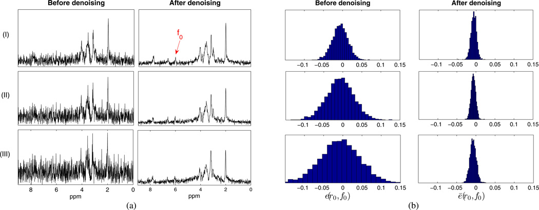
For PS-based low-rank filtering, in the case of high/moderate SNR (ideally as long as ∥E∥₂ ≤ λ_L (A₀) or in the range above 18 dB for the simulated ¹H MRSI dataset described in Section IV), we choose rank L₁ of C₀ according to (13). To evaluate the performance of the described rank selection method, we performed rank selection on the simulated dataset with true rank L₁ = 8. Specifically, we performed a Monte Carlo study with 9 different noise levels, 32 noise realizations per noise level, and estimated ∥E∥₂ using the Marchenko–Pastur distribution ([28]). The effective rank L̂₁ was selected according to (13). Fig. 7(a) shows some representative noisy spectra at the highest, medium, and lowest SNRs used in the experiment. For this experiment and the rest of this paper, we define SNR in terms of signal energy and signal amplitude as

$$\mathrm{S}\mathrm{N}{\mathrm{R}}_{\mathrm{e}}=10{\text{log}}_{10}\frac{{\parallel s_0\parallel }_2}{{\parallel s-s_0\parallel }_2}\mathrm{S}\mathrm{N}{\mathrm{R}}_{\mathrm{p}}=\frac{\text{amplitude of the largest peak}}{\text{standard deviation of the noise}}$$ (17)

where s and s₀ are the noisy and noiseless signals, respectively.

Fig. 7.

Monte Carlo study of low-rank filtering based on partial separability: (a) representative noisy and denoised spectra at three SNR levels; (b) error distributions calculated as the histograms of e and ē according to (21) at a particular location (r₀, f₀). For this illustrative example, r₀ is a representative voxel in the white matter region marked as “2” in Fig. 3(e) and f₀ is the frequency point marked in Fig. 7(a). Notice the reduced noise variances achieved by denoising.

Table I shows the mean effective rank L̄₁, averaged over all the noise realizations. Notice that ∥E∥₂ is closely estimated using the Marchenko–Pastur distribution at every SNR level, as can be seen from the reported relative error $\frac{\parallel \mathit{E}{\parallel }_2-\parallel \mathit{Ê}{\parallel }_2}{\parallel \mathit{E}{\parallel }_2}$. The results also show that as the SNR decreases, the discussed approach underestimates L₁. In practice, the choice of L₁ can also be guided by the known number of spectral components present in the spectrum [30].

TABLE 1.

Monte Carlo Experiment on Choosing Effective Rank L̄₁ at Nine Different SNR Levels

SNRe (s(k,t))	23.72	22.23	20.94	19.83	18.85	17.97	17.17	16.45	15.78
SNRe (s(f)) at voxel 1	6.42	5.17	4.45	3.83	3.26	2.83	2.27	1.99	1.86
SNRe (s(f)) at voxel 2	32.46	31.31	29.96	28.52	27.82	27.01	26.22	25.41	24.83
$\frac{\parallel \mathit{E}{\parallel }_2-\parallel \mathit{Ê}{\parallel }_2}{\parallel \mathit{E}{\parallel }_2}$	0.0057	0.0051	0.0053	0.0058	0.0046	0.0050	0.0054	0.0050	0.0058
L1	8	8	7.03	6.63	6.06	6.00	5.25	5.03	4.97

True rank L₁ = 8. Voxel 1 is in the region of low SNR, while voxel 2 is in the region of high SNR. All SNR values are reported in decibels.

For LP-based low-rank filtering, the choice of rank L₂ of matrix H₀ is based on the AIC criteria as specified in (14). We performed a Monte Carlo study on rank L₂ selection with the simulated dataset at 3 different noise levels, for each noise level 256 noise realizations were considered. The corresponding representative noisy spectra are shown in Fig. 8(a). Fig. 2 shows the computed mean AIC values (averaged over the noise realizations) as a function of candidate rank values. The effective rank L̂₂ is typically chosen to minimize AIC. However, this usually leads to an overestimated rank [29]. To achieve a closer estimate, we suggest choosing the rank to be the threshold point at which there is no significant reduction in the AIC value when the rank is further increased. In practice, the choice of L₂ can also be guided by the known number of spectral peaks present in the spectrum.

Fig. 8.

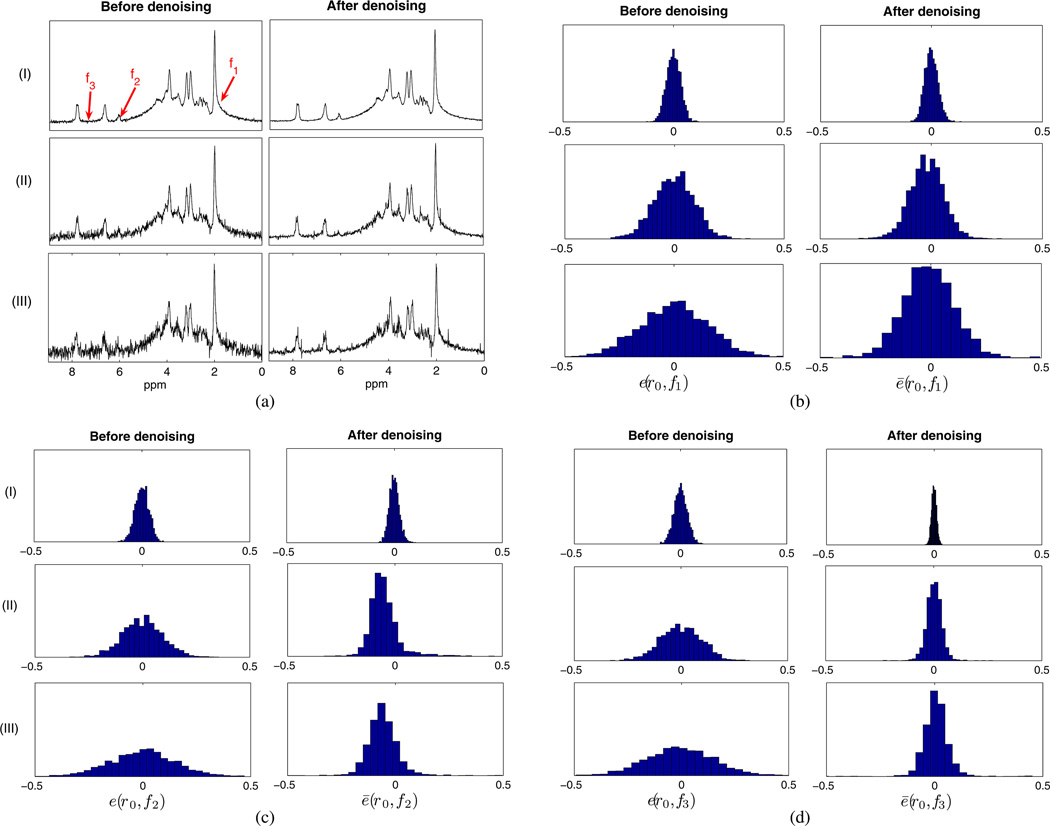
Monte Carlo study of low-rank filtering based on linear predictability: (a) representative noisy and denoised spectra at three noise levels; (b)–(d) error distributions calculated as the histograms of e and ē according to (21) at particular locations (r₀, f₁), (r₀, f₂), and (r₀, f₃), respectively. For this illustrative example, r₀ is a representative voxel in the white matter region marked as “2” in Fig. 3(f) and f₁, f₂, and f₃ are the frequency points marked in Fig. 8(a). Notice that the denoising performance is frequency dependent.

Fig. 2.

Monte Carlo study of rank L₂ selection based on AIC: top row shows the mean AIC value (averaged over 256 noise realizations) as a function of L̂₂ at (a) low noise level with SNR_e=26.61 dB and SNR_p=94.4; (b) medium noise level with SNR_e=17.03 dB and SNR_p=30.4; (c) high noise level with SNR_e=12.76 dB and SNR_p=17.9. The true rank L₂ in this experiment was 20.

Inaccurate rank estimation is more problematic for LP-based low-rank filtering than for PS-based low-rank filtering. Specifically, an overestimated rank L₂ (L̂₂ > L₂) can result in spurious peaks. Using an underestimated rank (without imposing the Hankel structure) can alleviate the problem. However, a highly underestimated rank L̂₂ can lead to a loss of useful spectral information, which is undesirable. Typically, peaks with small amplitudes are distorted or lost first [31]. Possible peak loss due to rank underestimation can be alleviated by not imposing the Hankel constraint as discussed in Section III-A. For PS-based low-rank filtering, severe rank underestimation can lead to spatial blurring and spectral line broadening. An overestimated rank L₁ in this case does not directly introduce bias and spurious peaks, but would reduce its filtering effectiveness.

IV. Results and Discussions

In this section, results from simulated and experimental data are presented to demonstrate the denoising performance of the proposed technique.

A. Simulations

We simulate a spatial-spectral distribution function based on literature values of ¹H metabolites and experimental data. We consider five commonly MR-observable metabolites in the human brain [24], [30]: N-acetylaspartate (NAA), creatine (Cr), choline (Cho), glutamate/glutamine (Glx), and myo-inositol (m-Ins). For each metabolite, a spectral profile was obtained from quantum mechanical simulations of a spin-echo MR experiment [32]. The spatial distribution of each metabolite was created based on commonly reported literature values from three segmented regions of cerebrospinal fluid, gray matter (GM), and white matter (WM) [30], [33], [34]. To evaluate the ability of the proposed method to handle nonideal conditions, Gaussian (instead of pure Lorentzian) lineshape was used with an additional baseline signal. Lineshape parameters were chosen based on commonly reported values in the literature [35], [36]. The baseline signal was extracted from single-voxel CSI PRESS experimental data of the brain with TE=30 ms. MRSI data were simulated at the magnetic field strength of 3 T with a spectral bandwidth of 1200 Hz and complex Gaussian noise was added.

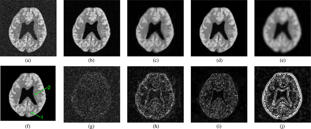
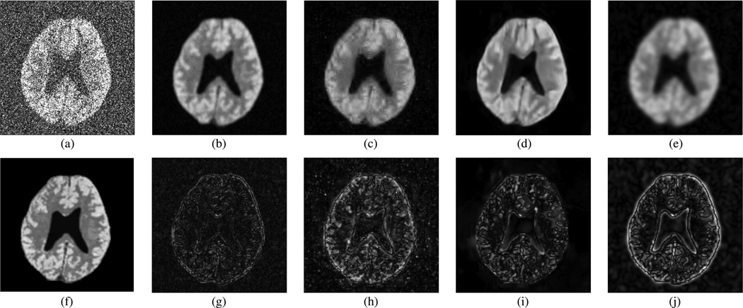
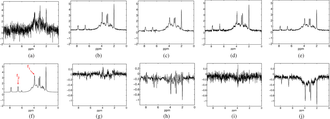
Figs. 3 and 4 show the spatial distribution of the spatialspectral function at a high SNR frequency of 3.94 ppm and a low SNR frequency of 6.66 ppm, both indicated in Fig. 5(f) as “f₁” and “f₂ ”, respectively. We compare the proposed approach with 3-D wavelet soft shrinkage (Daubechies 4-tap kernel filter, 4 levels), sparse 3-D transform-domain collaborative filtering [37] (code is available at http://www.cs.tut.fi/foi/GCFBM3D/), and conventional Gaussian apodization. The wavelet shrinkage threshold and apodization constant were chosen to yield the same level of the residual noise variance as that for the proposed approach (threshold T = 2.28σ₀). It can be clearly seen that the corresponding wavelet-denoised spatial-spectral function in Figs. 3(c) and 4(c) has an improved SNR at the expense of blurring the spatial features significantly, while the proposed denoising preserves the spatial features better. Collaborative filtering performed well at a high SNR frequency such as the one shown in Fig. 3, but at a lower SNR frequency shown in Fig. 4 the spatial features such as edges in the GM region were smoothed out noticeably by the collaborative filtering while the residual noise variance in the denoised spectrum was larger than that of obtained from LORA [see Fig. 5(d)]. Gaussian apodization shown in Figs. 3(e) and 4(e) has the poorest tradeoff between SNR and resolution among all methods, as expected.

Fig. 3.

Denoising results—spatial distributions ρ(r, f₁) at a SNR frequency [3.94 ppm; see Fig. 5(f)] obtained from (a) noisy data; (b) LORA denoising; (c) wavelet denoising; (d) sparse 3-D transform-domain collaborative filtering; (e) Gaussian apodization; and (f) noiseless data. Corresponding errors of (b)–(e) are shown in (g)–(j), respectively.

Fig. 4.

Denoising results—spatial distributions ρ(r, f₂) at a low-SNR frequency [6.66 ppm; see Fig. 5(f)], obtained from (a) noisy data; (b) LORA denoising; (c) wavelet denoising; (d) sparse 3-D transform-domain collaborative filtering; (e) Gaussian apodization; and (f) noiseless data. Corresponding errors of (b)–(e) are shown in (g)–(j), respectively.

Fig. 5.

Denoising results—spectra at a particular voxel, marked as “1” in Fig. 3(f), obtained from (a) noisy data; (b) LORA denoising; (c) wavelet shrinkage; (d) sparse 3-D transform-domain collaborative filtering; (e) Gaussian apodization; and (f) noiseless data. Corresponding errors of (b)–(e) are shown in (g)–(j), respectively. All spectra are shown in the real-valued mode.

Fig. 5 shows representative spectra from a particular voxel marked as “1” in Fig. 3(f). Both Gaussian apodization and wavelet denoising improve the SNR at an expense of line broadening and loosing metabolite amplitudes, with Gaussian apodization performing the worst. This amplitude loss can be seen from the corresponding residual spectra, which are not centered at zero, as shown in Fig. 5(h) and (j).

B. Denoising Performance

To analyze the denoising performance of the proposed low-rank filtering, we rewrite C and C̄as C = C₀ + E and C̄ = C₀ +Δ, where C₀ is an N × M data matrix with rank L₁ as described in (5), E is the noise matrix, C̄ is formed from the denoised data as obtained from (15), and Δ is the residual error, which can contain both residual noise and possible signal loss due to low-rank filtering.Without loss of generality, we assume M < N. The denoised matrix C̄ is obtained according to (15). We define the noise reduction factor as

$$g=\frac{{\parallel \mathit{E}\parallel }_F}{{\parallel \mathbf{\Delta }\parallel }_F}.$$ (18)

By defining the SNR before and after denoising as $20{\text{log}}_{10}\frac{{\mathrm{P}}_{\mathrm{s}}}{\parallel \mathit{E}{\parallel }_F}$ and $20{\text{log}}_{10}\frac{{\mathrm{P}}_{\mathrm{s}}}{\parallel \mathbf{\Delta }{\parallel }_F}$, where P_s denotes the signal power, the SNR gain can be calculated as 20 log₁₀ g. Ideally, one would want g = ∞. In the full-rank case when L₁ = M and no denoising is achieved, g is equal to 1.

Computing g as in (18) requires knowing the ground truth in order to compute ∥Δ∥_F. However, notice that we only need to estimate the norm ∥Δ∥_F rather than knowing Δ completely. Thus, one would hope that there is a signal-independent expression to predict ∥Δ∥_F closely. In general, it is hard to accurately characterize singular values of C₀ ,C, and C̄. However, under assumptions that:

Cond1: the signal and noise (before and after denoising) subspaces are uncorrelated in the sense that C₀^H E = 0 and C₀^HΔ = 0;

Cond2: the noise is complex white, i.e., E^HE and Δ^H Δ are scalar multiples of identity matrix [38]; we can obtain the following approximate formula based on the theoretical results of SVD of noisy matrices in [38]:

$$g=\sqrt{\frac{{\sum }_{i=1}^M{\lambda }_i^2(\mathit{E})}{{\sum }_{i=1}^{{\mathrm{L̂}}_1}{\lambda }_i^2(\mathit{E})}},\text{if}{\mathrm{L̂}}_1\ge L_1.$$ (19)

Expression (19) provides a signal-independent prediction of g. It suggests that 1) in the case of accurate rank estimation (L̂₁ = L₁) and λ_i(E) are all equal, the noise reduction factor is of the order of $\sqrt{\frac{M}{{\mathrm{L̂}}_1}}$; 2) in the case of overestimated rank (L̂₁ > L₁), the residual noise level is larger than the residual noise level with correct rank determination. In practice, the conditions (Cond1) and (Cond2) which are required for (19) to hold are never satisfied exactly. However, we observed that a mild violation of these conditions may still give a rough guess of g, as shown in our simulation study discussed below.

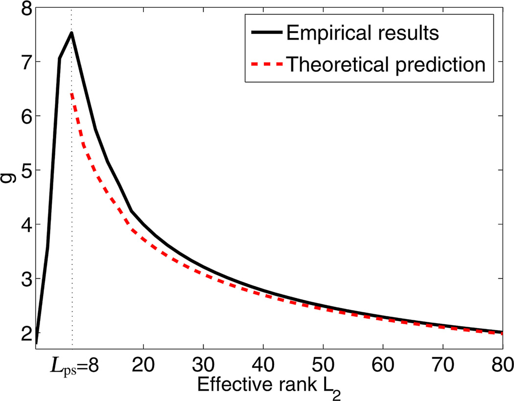
Based on the simulated ¹H MRSI dataset described in Section IV-A, we performed a Monte Carlo study to compute g according to (18), averaged over 32 noise realizations. The noise reduction factor g is plotted as a function of the estimated rank L̂₁ in Fig. 6.We observe that when the rank is properly chosen, g reaches its maximum value (about 7.6 for the simulated dataset). As the rank is overestimated (L̂₁ > L₁) and approaches the full rank, g decreases to 1, as expected. The reduction of g reflects the residual noise variance in the overestimated rank case and the signal loss in the underestimated rank case. A nice feature of this plot is that it shows how much of the noise reduction we can achieve even in the case when the rank is incorrectly estimated. For example, if the rank was overestimated to be 32, while the true rank is 8, then according to this plot, we still achieve a factor of about 3 (or 9.5 dB) of improvement in the SNR. Thus, for the sake of improving SNR, estimating rank precisely is not a critical point, as long as we do not underestimate the rank causing the signal loss. Note that with the considered dataset in Fig. 6, the relative error $\frac{\parallel {\mathit{E}}^H\mathit{E}-M{\sigma }_0^2\mathit{I}{\parallel }_F}{M{\sigma }_0}=0.99$ for condition (Cond1) and $\frac{\parallel {\mathit{C}}_0^H\mathit{E}{\parallel }_F}{\sqrt{\parallel {\mathit{C}}_0^H{\mathit{C}}_0{\parallel }_F\parallel {\mathit{E}}^H\mathit{E}{\parallel }_F}}=0.15$ for condition (Cond2). These numbers did not significantly change as the SNR was varied from low to high [see Fig. 7(a)] for representative SNR levels. Conditions (Cond1) and (Cond2) for Δ are satisfied closer as L̂ approaches M. Predicted value from (19) is plotted in the same figure as the empirical value of g in Fig. 6. Notice that in the region L̂₁ > L₁ the theoretically predicted values of g approach its empirical value as L̂₁ tends to the full-rank case.

Fig. 6.

Noise reduction factor g for low-rank filtering based on partial separability as a function of the estimated rank L̂₁. Empirical values of g (black) and corresponding theoretical approximations (red) were computed according to (18) and (19), respectively. The true rank L₁ = 8. Notice that in the region L̂₁ > L₁, the theoretically predicted values of g tend to its empirical values and both approach 1 in the full-rank case.

We have performed a similar analysis on the noise reduction factor g, for the case of low-rank filtering of linear prediction matrix. However, to evaluate the level of SNR improvement for low-rank filtering of linear prediction matrix, we rather define the following factor:

$$h=\frac{{\parallel \mathit{\xi }\parallel }_2}{{\parallel \mathit{\eta }\parallel }_2}$$ (20)

where ξ and η are vectors extracted from the first row and last column of E and Δ, respectively. We performed a Monte Carlo study with 256 noise realizations to compute h at different noise levels shown in Fig. 8(a). The reduction factor h depends on the conditioning of the Hankel matrix H₀. For the case considered here, we observed that h achieves the value of around 1.7. However, for better-conditioned cases with well-separated spectral peaks, h can be significantly bigger (in the range of 5 for a spectrum with three peaks, separated by 0.57 ppm). This experiment suggests that LP-based low-rank filtering can be less effective than PS-based low-rank filtering, although both are used in LORA.

We performed a Monte Carlo study to further evaluate the denoising effectiveness of low-rank filtering with 2048 noise realizations to obtain histograms of the errors before and after denoising as

$$e=s-s_0ē=\mathrm{s̄}-s_0$$ (21)

where s̄ denotes the denoised data. Fig. 7 shows some representative results or the low-rank filtering based on partial separability. It is easy to see that a significant reduction in the noise variance was achieved at every SNR level. Note that low-rank filtering is a “biased” estimator. However, the resulting bias is negligible once the rank is correctly chosen and SNR is not extremely low. In the case of extremely low SNR, using an overestimated rank reduces bias, but at the expense of reduced filtering effect.

Fig. 8 shows some representative results from a Monte Carlo study of low-rank filtering based on linear predictability. Notice that the denoising performance is frequency dependent. Histogram at a low SNR frequency f₂ in Fig. 8(c) shows that a significant noise variance reduction is still achieved; however, a larger bias is introduced, compared to the case of a higher SNR frequency f₁ in Fig. 8(b). For the frequency regions that contain mostly noise (such as the frequency f₃ in [Fig. 8(d)], we observe significant noise variance reduction with no bias.

C. In Vivo Experiments

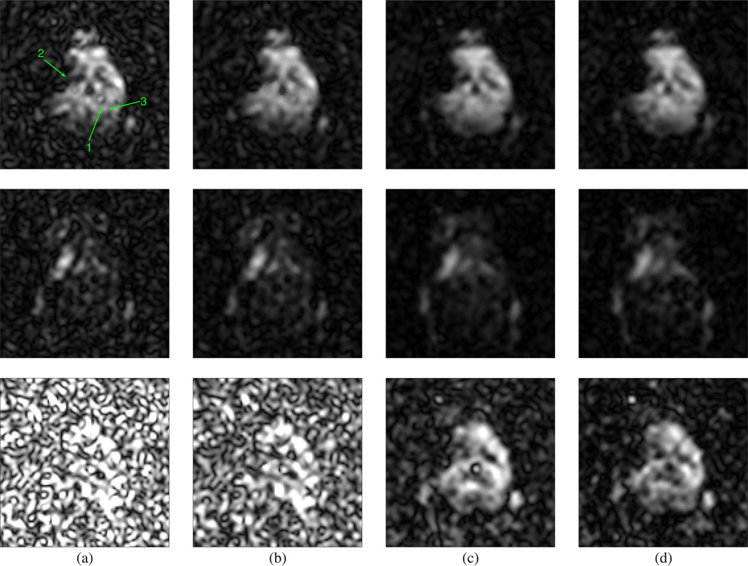
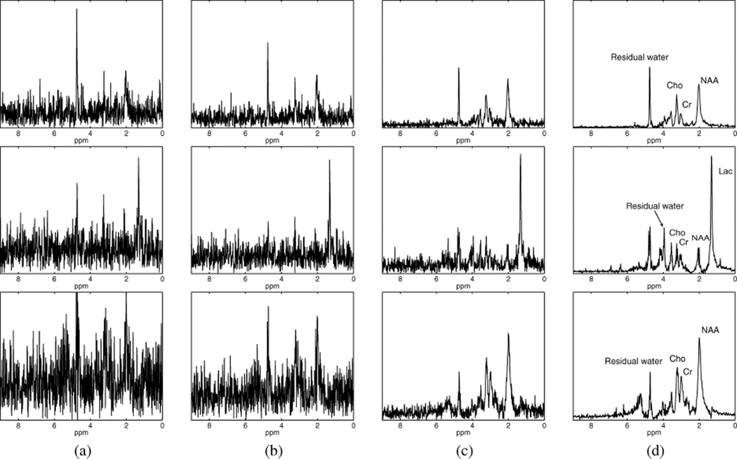
We have applied LORA to denoise in vivo MRSI data of the mouse brain, acquired using a Varian INOVA 11.74 T (500 MHz) MRI scanner at Washington University in St. Louis. This dataset was previously described and used in [39]. A craniectomy was performed on the mouse and the middle cerebral artery (MCA) was electrocoagulated. In vivo MRSI data were acquired using a CSI sequence with chemical shift selective suppression (CHESS) water suppression, TE=270 ms, TR=1500 ms, bandwidth=6000 Hz, 1024 FID data points, and 8 averages. The CSI dataset was preprocessed to compensate for field inhomogeneity and remove water resonance using HSVD [3]. Notice that the residual water and artifacts from field inhomogeneity were not completely removed. For a detailed description of the dataset, see [39]. Before performing LORA denoising, data were preprocessed with spatial denoising using anatomical reconstruction [40] to protect spatial features from field inhomogeneity artifacts during the low-rank filtering due to spatiotemporal partial separability. NAA, lactate (Lac), and glutamate/glutamine (Glx) spatial maps were obtained by integrating the complex spectrum at 2.02 ppm, 1.33 ppm, and in the region from 2.7 to 2.8 ppm, respectively. Fig. 9 shows NAA and Lac maps obtained from the measured, spatially denoised, and LORA-denoised data after each individual low-rank filtering. Fig. 10 shows spectra obtained from these reconstructions at voxels outside of electrocogualation area (voxels marked as “1” and “3” in [Fig. 9(a)]) and in the region of electrocogualation (voxel marked as “2” in [Fig. 9(a)]). It can be clearly seen that the noise has been significantly suppressed. Electrocoagulation blocked MCA, resulting in a stoppage of blood supply and lack of oxygen. Thus, we expect elevated Lac and reduced NAA concentrations in the electrocogualation region, which can be seen from the LORA-denoised reconstruction in Fig. 9(d).

Fig. 9.

Denoising results from in vivo experimental data. Spatial distributions corresponding to NAA in the region from 1.9 to 2.1 ppm (top row), Lac in the region from 1.2 to1.37 ppm (middle row), and Glx in the region from 2.7 to 2.8 ppm (bottom row) obtained from (a) noisy data; (b) spatial denoising; (c) PS-based low-rank filtering; (d) LP-based low-rank filtering of the results in (c) (the final output of LORA).

Fig. 10.

Denoising results from in vivo experimental dataset: spectra at three voxels in the region outside of electrocogualation (voxel 1, top row, and voxel 3, bottom row) and inside of electrocogualation area (voxel 2, middle row), obtained from (a) noisy data; (b) spatial denoising; (c) PS-based low-rank filtering of the spatial filtering results; (d) LP-based low-rank filtering of PS-based low-rank filtering results (which is the final output of LORA). All spectra are shown in absolute mode and on the same scale.

It is also interesting to observe the filtering results of each individual filtering step. While spatial filtering is useful, its output is often still too noisy for practical application. The results were significantly improved by subsequent PS-based and LP-based low-rank filterings. Note that while PS-based low-rank filtering performs spatial-spectral denoising, LP-based low-rank filtering is just a spectral filter. These filtering characteristics can be clearly observed from Figs. 9 and 10. Note also that the denoised spectra in Fig. 10(d) show minimal spectral distortions with impressive SNR improvement as compared to the results in Fig. 10(a).

V. Conclusion

This paper has presented a new method (LORA) for spatialspectral filtering of MR spectroscopic imaging data. LORA exploits the low-rank properties of MRSI data, one due to partial separability and the other due to linear predictability. The combined use of partial separability and linear predictability provides a new principled way to improve SNR for spatiotemporal imaging. Simulation and experimental results demonstrate that LORA can effectively denoise MRSI data with very low SNRs. It should prove useful for practical MRSI applications.

Biographies

Hien M. Nguyen received the B.S. degree in computer science from the Hanoi University of Technology, Hanoi, Vietnam, in 2002, and the M.S. and Ph.D. degrees in electrical and computer engineering from the University of Illinois at Urbana-Champaign, Champaign, IL, in 2007 and 2011, respectively.

She is currently a Postdoctoral Researcher in the Department of Radiology, Richard M. Lucas Center for Imaging, Stanford University, Stanford, CA. Her research interests include multidimensional signal processing, parameter estimation, and inverse problems, with particular emphasis on biomedical imaging applications.

Xi Peng received the B.Eng. and M.S. degrees in measurement, control, and instruments, and the Ph.D. degree in electrical engineering all from Wuhan University, Hubei, China, in 2006, 2008, and 2012, respectively.

During the doctoral process, he was a Visiting Scholar in Beckman Institute, University of Illinois at Urbana-Champaign. He is currently an Assistant Professor in the Paul C. Lauterbur Research Center for Biomedical Imaging, Institute of Biomedical and Health Engineering, Shenzhen Institutes of Advanced Technology, Chinese Academy of Sciences, Shenzhen, China. His research interests include image reconstruction, parameter estimation, and signal processing for biomedical applications.

Minh N. Do received the Dr.Sci. degree in communication systems from the Swiss Federal Institute of Technology Lausanne (EPFL), Zurich, Switzerland, in 2001.

He is currently an Associate Professor in the Department of Electrical and Computer Engineering, University of Illinois at Urbana, Champaign, Urbana. His research interests include image and multidimensional signal processing, wavelets and multiscale geometric analysis, computational imaging, augmented reality, and visual information representation.

Prof. Do received a Silver Medal from the 32nd International Mathematical Olympiad in 1991, a University Medal from the University of Canberra in 1997, a Doctorate Award from the EPFL in 2001, a CAREER Award from the National Science Foundation in 2003, and a Young Author Best Paper Award from the IEEE in 2008. He is a member of the IEEE Signal Processing Theory and Methods and Image, Video, and Multidimensional Signal Processing Technical Committees, and an Associate Editor of the IEEE Transactions on Image Processing.

Zhi-Pei Liang (M’92–SM’98–F’06) received the Ph.D. degree in biomedical engineering from Case Western Reserve University, Cleveland, OH, in 1989.

He is currently the Franklin W. Woeltge Professor of Electrical and Computer Engineering at the University of Illinois at Urbana-Champaign (UIUC), Champaign, IL. His research interests include image formation theory, algorithms, and biomedical applications.

Dr. Liang is a recipient of the 1990 Sylvia Sorkin Greenfield Best Paper Award (Medical Physics), an National Science Foundation’s CAREER Award (1995), and the 1999 IEEEEMBS Early Career Achievement Award, and the 2012 International Federation for Medical and Biological Engineering Otto Schmitt Award. He was named Henry Magnuski Scholar (1999–2001), and University Scholar (2001–2004) at UIUC. He is a fellow of the International Society for Magnetic Resonance in Medicine (2010), and was elected to the American Institute for Medical and Biological Engineering in 2005 and to the International Academy of Medical and Biological Engineering in 2012. He served as President of the IEEE Engineering in Medicine and Biology Society from 2011 to 2012.

References

- 1.de Graaf RA. In Vivo NMR Spectroscopy. 2nd ed. New York: Wiley; 2007. [Google Scholar]
- 2.Costanzo AD, Trojsi F, Tosetti M, Schirmer T, Lechner SM, Popolizio T, Scarabino T. Proton MR spectroscopy of the brain at 3 T: An update. Eur. Radiol. 2007;vol. 17:1651–1662. doi: 10.1007/s00330-006-0546-1. [DOI] [PubMed] [Google Scholar]
- 3.van den Boogaart A, van Ormondt D, Pijnappel WWF, de Beer R, Ala-Korpela M. Removal of the water resonance from 1H magnetic resonance spectra. In: McWhirter JG, editor. Mathematical Signal Processing III. Oxford: Clarendon Press; 1994. pp. 175–195. [Google Scholar]
- 4.de Greiff HFC, Ramos-Garcia R, Lorenzo-Ginori JV. Signal denoising in magnetic resonance spectroscopy using wavelet transforms. Concepts Magn. Reson. 2002;vol. 14:388–401. [Google Scholar]
- 5.Andrews HC, Patterson CL. Singular value decompositions and digital image processing. IEEE Trans. Acoust. Speech Sign. Process. 1976 Feb;vol. 24(no. 1):26–53. [Google Scholar]
- 6.Kumaresan R, Tufts DW. Estimating the parameters of exponentially damped sinusoids and pole-zero modeling in noise. IEEE Trans. Acoust., Speech, Signal Process. 1982 Dec;vol. 30(no. 6):833–840. [Google Scholar]
- 7.Buades A, Coll B, Morel JM. A review of image denoising algorithms, with a new one. Multiscale Model. Simul. 2005;vol. 4:490–530. [Google Scholar]
- 8.Ahmed OA. New denoising scheme for magnetic resonance spectroscopy signals. IEEE Trans. Med. Imag. 2005 Jun;vol. 24(no. 6):809–816. doi: 10.1109/TMI.2004.828350. [DOI] [PubMed] [Google Scholar]
- 9.Diop A, Zaim-Wadghiri Y, Briguet A, Graveron-Demilly D. Improvements of quantitation by using the Cadzow enhancement procedure prior to any linear-prediction methods. J. Magn. Reson. 1994;vol. 105:17–24. [Google Scholar]
- 10.Beer RD. Quantitative in vivo NMR. Univ. Technol. Delft Lect. Notes; 1994. [Online]. Available: http://www.intermnet.ua.es/inteRMNet/c59/index.html. [Google Scholar]
- 11.Sava AC, Sima D, Poullet J, Huffel SV. Exploiting spatial information for estimating metabolite concentration in MRSI. Proc. 17th Int. Soc. Mag. Reson. Med. 2009 [Google Scholar]
- 12.Bao Y, Maudsley AA. Improved reconstruction for MR spectroscopic imaging. IEEE Trans. Med. Imag. 2007 May;vol. 26(no. 5):686–695. doi: 10.1109/TMI.2007.895482. [DOI] [PMC free article] [PubMed] [Google Scholar]
- 13.Kornak J, Young K, Schuff N, Maudsley AA, Weiner MW. Bayesian reconstruction of low resolution magnetic resonance imaging modalities. Proc. Leeds Annu. Stat. Res. Workshop—Bioinformat. Imag. Wavelets. 2004:89–92. [Google Scholar]
- 14.Cadzow JA. Signal enhancement—A composite property mapping algorithm. IEEE Trans. Acoust. Speech Sign. 1988 Jan;vol. 36(no. 1):49–62. [Google Scholar]
- 15.Eslami R, Jacob M. Reduction of distortions in MRSI using a new signal model. Proc. IEEE Int Symp. Biomed. Imag. 2009 Jun-Jul;:438–441. [Google Scholar]
- 16.Nguyen HM, Haldar JP, Do MN, Liang Z-P. Denoising of MR spectroscopic imaging data with spatial-spectral regularization. Proc. IEEE Int. Symp. Biomed. Imag. 2010 Apr;:720–723. [Google Scholar]
- 17.Liang Z-P. Spatiotemporal imaging with partially separable functions. Proc. IEEE Int. Symp. Biomed. Imag. 2007 Apr;:988–991. [Google Scholar]
- 18.Nguyen HM, Peng X, Do MN, Liang Z-P. Spatiotemporal filtering of MR spectroscopic imaging data by low-rank approximations. Proc. IEEE Int. Symp. Biomed. Imag. 2011 Mar-Apr;:857–860. [Google Scholar]
- 19.Peng X, Nguyen H, Haldar J, Hernando D, Wang X-P, Liang Z-P. Correction of field inhomogeneity effects in limited k-space coverage MRSI data with anatomical constraint. Proc. Int. Soc. Mag. Reson. Med. 2010:883–886. doi: 10.1109/IEMBS.2010.5627873. [DOI] [PubMed] [Google Scholar]
- 20.Bashir A, Yablonskiy DA. Natural linewidth chemical shift imaging (NL-CSI) Mag. Res. Imag. 2006 Jul;vol. 56:7–18. doi: 10.1002/mrm.20917. [DOI] [PMC free article] [PubMed] [Google Scholar]
- 21.Khalidov I, Ville DVD, Jacob M, Lazeyras F, Unser M. BSLIM: Spectral localization by imaging with explicit B0 field inhomogeneity compensation. IEEE Trans. Med. Imag. 2007 Jul;vol. 26(no. 7):990–1000. doi: 10.1109/TMI.2007.897385. [DOI] [PubMed] [Google Scholar]
- 22.Hu X, Levin DN, Lauterbur PC, Spraggins T. SLIM: Spectral localization by imaging. Magn. Reson. Med. 1988;vol. 8:314–322. doi: 10.1002/mrm.1910080308. [DOI] [PubMed] [Google Scholar]
- 23.Liang Z-P, Lauterbur PC. A theoretical analysis of the SLIM technique. J. Magn. Reson. 1993;vol. 102:54–60. [Google Scholar]
- 24.Barker PB, Lin DDM. In vivo proton MR spectroscopy of the human brain. Prog. NMR Spect. 2006;vol. 49:99–128. [Google Scholar]
- 25.Seeger U, Klose U. Parameterized evaluation of macromolecules and lipids in proton MR spectroscopy of brain diseases. Magn. Reson. Med. 2003;vol. 49:19–28. doi: 10.1002/mrm.10332. [DOI] [PubMed] [Google Scholar]
- 26.Pijnappel WWF, van den Boogaart A, de Beer R, van Ormondt D. SVD-based quantification of magnetic resonance signals. J. Magn. Reson. 1992;vol. 97:122–134. [Google Scholar]
- 27.Iohvidov IS. Hankel and Toeplitz Matrices and Forms. Birkhauser; 1982. [Google Scholar]
- 28.Marcenko VA, Pastur LA. Distribution of eigenvalues for some sets of random matrices. Math. USSR—Sb. 1967;vol. 1:457–483. [Google Scholar]
- 29.Shibata R. Selection of the order of an autoregressive model by Akaike’s information criterion. Biometrika. 1976;vol. 63:117–126. [Google Scholar]
- 30.Govindaraju V, Young K, Maudsley AA. Proton NMR chemical shifts and coupling constants for brain metabolites. NMR Biomed. 2000;vol. 13:129–153. doi: 10.1002/1099-1492(200005)13:3<129::aid-nbm619>3.0.co;2-v. [DOI] [PubMed] [Google Scholar]
- 31.Bazan FSV, Toint PL. Conditioning of infinite Hankel matrices of finite rank. Syst. Control Lett. 2000;vol. 41:347–359. [Google Scholar]
- 32.Soher BJ, Young K, Bernstein A, Aygula Z, Maudsley AA. GAVA: Spectral simulation for in vivoMRS applications. J. Magn. Reson. 2007;vol. 185:291–299. doi: 10.1016/j.jmr.2007.01.005. [DOI] [PMC free article] [PubMed] [Google Scholar]
- 33.Srinivasan R, Sailasuta N, Hurd R, Nelson S, Pelletier D. Evidence of elevated glutamate in multiple sclerosis usingmagnetic resonance spectroscopy at 3 T. Brain. 2005;vol. 128:1016–1025. doi: 10.1093/brain/awh467. [DOI] [PubMed] [Google Scholar]
- 34.Wang Y, Li S-J. Differentiation of metabolic concentrations between gray matter and white matter of human brain by in vivo1 H magnetic resonance spectroscopy. Magn. Reson. Med. 1998;vol. 39:28–33. doi: 10.1002/mrm.1910390107. [DOI] [PubMed] [Google Scholar]
- 35.Traber F, Block W, Lamerichs R, Gieseke J, Schild HH. 1H metabolite relaxation times at 3.0 Tesla: Measurements of T1 and T2 values in normal brain and determination of regional differences in transverse relaxation. J. Magn. Reson. Imag. 2004;vol. 19:537–545. doi: 10.1002/jmri.20053. [DOI] [PubMed] [Google Scholar]
- 36.Choi C, Coupland NJ, Bhardwaj PP, Kalra S, Casault CA, Reid K, Allen PS. T2 measurement and quantification of glutamate in human brainin vivo. Magn. Reson. Med. 2006;vol. 56:971–977. doi: 10.1002/mrm.21055. [DOI] [PubMed] [Google Scholar]
- 37.Dabov K, Foi A, Katkovnik V, Egiazarian K. Image denoising by sparse 3D transform-domain collaborative filtering. IEEE Trans. Image Process. 2007 Aug;vol. 16(no. 8):2080–2095. doi: 10.1109/tip.2007.901238. [DOI] [PubMed] [Google Scholar]
- 38.Moor BD. The singular value decomposition and long and short spaces of noisy matrices. IEEE Sign. Process. 1993 Sep;vol. 41(no. 9):2826–2838. [Google Scholar]
- 39.Haldar JP, WU T-H, Wang Q, Chen C-I, Song S-K, Liang Z-P. Further development in anatomically constrained MR image reconstruction: Application to multimodal imaging of mouse stroke. Proc. Int. IEEE Eng. Med. Biol. Soc. 2008 Aug;:422–425. doi: 10.1109/IEMBS.2008.4649180. [DOI] [PubMed] [Google Scholar]
- 40.Haldar JP, Hernando D, Song S-K, Liang Z-P. Anatomically constrained reconstruction from noisy data. Magn. Reson. Med. 2008;vol. 59:810–818. doi: 10.1002/mrm.21536. [DOI] [PubMed] [Google Scholar]