A New Tool for Quantifying and Characterizing Asymmetry in Bilaterally Paired Structures

Abstract

This paper introduces a new tool to quantify and characterize asymmetry in bilaterally paired structures. This method uses deformable registration to produce a dense vector field describing the point correspondences between two images of bilaterally paired structures. The deformation vector field properties are clustered to detect and describe regions of relevant asymmetry. Three methods are provided to analyze the asymmetries: the global asymmetry score uses cluster features to quantify overall asymmetry, the local asymmetry score quantifies asymmetry in user-defined regions of interest, and the asymmetry similarity measure quantifies pairwise similarity of individual asymmetry. The scores and image distances generated by this tool are shown to correlate highly with asymmetry ratings assigned by an expert.

I. INTRODUCTION

Human faces are almost never perfectly symmetric. However, in some individuals the asymmetry can be quite marked, which is clinically referred to as craniofacial microsomia. The condition usually involves underdevelopment, or hypoplasia, of the midface (upper jaw and nose), the lower jaw (or mandible), as well as positioning and/or malformation of the ear. The cause of this relatively common anomaly remains unknown, although both genetic and non-genetic factors are believed to contribute to the presentation. In the rarer familial cases, there is no consistency in the side of the face most affected. Research into the causes of craniofacial microsomia has been considerably hindered by the lack of appropriate animal models with the condition. However, we recently identified a number of new mutant mouse lines that exhibit fluctuating facial asymmetry involving both the upper and lower jaw and ears, similar to that seen in patients with craniofacial microsomia. These mice therefore represent excellent models for understanding the pathogenetic mechanisms of this condition. In mammals, the lower jaw bone is comprised of bilaterally paired hemi-mandibles. In humans, these fuse at the anterior midline by the end of the first year of postnatal life. However, in mice a cartilaginous join typically persists that allows the paired hemi-mandibles to be easily separated postmortem or digitally post-imaging. The aim of this work was to develop a tool by which asymmetry between hemi-mandibles and other bilaterally paired structures can be quantified and the spatial distribution of asymmetry assessed and compared across individuals. The tool introduced in this work will therefore aid research into the developmental basis of this condition and the specific role of the causative gene(s) and non-genetic factors.

II. RELATED WORK

In a previous work of ours, deformable registration was used to produce a dense vector field describing the point correspondences between two images, from which features were extracted to find regions of organized differences that were biologically relevant [6]. These methods were shown to detect regions of difference when evaluated on 3D images of chick embryonic faces warped with small magnitude deformations in regions critical to midfacial development.

Deformation morphology techniques have also proven useful in assessing symmetry. Deformation Based Asymmetry (DBA), a method for detecting asymmetry in brains was introduced in [4]. In this study, an average image from all subjects was created for the left and right hemispheres. One average hemisphere image was mirrored and warped to the other to estimate spatial differences between them. The asymmetry at a point was defined as the ratio of the displacement vector magnitude to the estimated within-group warping variance at that point. The proportion of d-values above a fixed level was used to test for overall asymmetry.

In [1], an individual map of brain symmetry was computed by deformably registering an image to itself mirrored over the line of symmetry. For group comparisons, all brain images were deformably registered to a symmetrical template created by mirroring a reference image across its symmetry plane. Statistical tests were then performed at each point on the template to assess group symmetry.

A similar method has been applied to assess craniofacial symmetry in a mouse model [5]. A symmetric atlas was generated by mirroring an average image across the midsagittal plane and registered to each subject in a group. The asymmetry measure was defined as the difference in magnitude of the deformation vectors at corresponding points on the left and right side of the symmetry plane. This method was also applied to CT images of human mandibles in [3].

III. DATA AND PREPROCESSING

The data used to test the methods presented in this work consists of 23 microCT scan datasets of adult mouse mandibles ranging from subtly asymmetric to significantly asymmetric. The scans included a similar number of male and female animals, all approximately 28–30 days old to reduce effects of age on size and shape. The scans were performed at an isotropic resolution of 18 microns, then each dataset reduced by a factor of 3 to simplify data handling and computation time. To quantify the symmetry of the mandibles, the external contour of each hemi-mandible was first extracted from the image. Our method based on geodesic active contours [6] was used to remove scan noise in the images, clarify indistinct borders between the object and the background, and to fill gaps and holes. Once the contours were extracted, the left hemi-mandibles were mirrored to permit comparison to the right sides and an affine transformation applied to align the images and remove pose differences.

IV. METHODOLOGY

The goal of the tool presented in this work is to provide a flexible way to analyze the asymmetries between bilaterally paired structures – in this case, the left and right hemi-mandible of individual mice, and to compare these asymmetries pairwise across individuals. This tool provides three primary modes of analysis:

1. the global asymmetry measure quantifies asymmetry across the surface of the mandible for an individual,

2. the local asymmetry measure quantifies asymmetry at user-defined regions of interest,

3. the asymmetry similarity measure quantifies pairwise similarity of individual asymmetry.

A. Deformable Registration

The first step in this method is a deformable registration that is applied to assess local differences at every point between aligned images of an individual’s right and mirrored left mandible. This registration determines the spatial transform mapping points from a source to homologous points on an object in a target image. The output is a dense deformation vector field in which the vector at each point describes the spatial transformation of that point. When applied to two images, these vectors reflect the structural differences between the source and target images. For this application, a B-spline deformable transform using a mutual information metric was chosen, since it is widely applicable and computationally efficient [2].

B. Vector Field Features

To interpret the deformation vectors in a meaningful way, it is necessary to identify and quantify regions of biologically relevant differences. For this application, two low-level vector properties were chosen: the deformation vector magnitude and the cosine distance between the deformation vector and the surface normal vector.

C. Clustering and Cluster Features

The two low-level features are individually clustered to find regions with similar transformation properties. Our spatially constrained K-means clustering algorithm described in [6] is used to identify the regions for each low-level feature. Asymmetric clusters are defined as those with an average deformation magnitude greater than T, where T is one standard deviation above the mean deformation magnitude of all voxels. The cluster features used to generate the feature vector are the: 1) location of cluster center, 2) number of voxels in cluster, 3) average magnitude value, and 4) average normal angle difference.

Each feature is normalized over the data set to remove differences in scale and distribution so that one feature does not dominate the feature vector.

D. Global Asymmetry Score

The first analysis method provided by this tool is the global asymmetry score. This score is used to quantify the magnitude of the deformation between the left and right hemi-mandibles. The goal was to produce scores that would correlate highly with the ratings assigned by an expert. It was necessary to use a more flexible method than a simple metric like the average energy of the transformation, because the expert ranking incorporates prior knowledge such as the relative importance of small regions of high magnitude differences and the need to exclude specific regions, such as the teeth because of variation due to wear. The global symmetry score provides the user with the ability to include this information in the scores. The score is calculated using only deformation magnitude cluster features, since the direction of the deformation was not used in the expert rankings. The two global magnitude features used are: 1) U_max, the maximum cluster mean, and 2) V_def, the total number of voxels in clusters with mean higher than the threshold T, where T is one standard deviation above the mean deformation magnitude of all voxels. These global features are normalized over the data set and the score is defined as:

$$S_{\mathit{\text{global}}}=\alpha U_{\mathit{\text{max}}}+(1-\alpha )V_{\mathit{\text{def}},}$$ (1)

where α is a constant specifying the contribution of the maximum deformation relative to the overall deformation. The value of this constant is specific to the application and allows the user to incorporate prior knowledge about the relative importance of small regions with high magnitude transformations compared to larger regions with smaller magnitude transformations. In addition, the tool allows clusters with a center in a region selected by the user to be excluded, for example, if deemed not to be biologically relevant to the particular question being considered.

E. Local Asymmetry Score

The local asymmetry score is a second asymmetry measure that provides an additional way to add prior knowledge to the symmetry score. The local asymmetry score uses only features from the deformation vectors in a neighborhood around the landmark points placed by an expert. The local asymmetry score is defined as

$$S_{\mathit{\text{local}}}=\alpha N_{\mathit{\text{max}}}+(1-\alpha )N_{\mathit{\text{average}},}$$ (2)

where N_max is maximum neighborhood average, N_average is the average deformation magnitude over all neighborhoods, and α is a constant specifying the significance of the maximum deformation versus overall deformation.

F. Similarity of Asymmetry

The third analysis method provided by this tool is a similarity measure to compare asymmetry across individuals, allowing individuals with similar shape and magnitude of asymmetry to be identified. This metric can be used on either the deformation magnitude or normal angle difference clusters, so they can be evaluated independently. The similarity is calculated by comparing the set of cluster feature vectors for each mandible. To allow for multiple types of queries, the user is also allowed to choose features from the feature vector to exclude for a specific query. To compare a mandible i to a second mandible j, the minimum distance from each cluster k in mandible i to a cluster in mandible j is found using

$$c_{i,k}=\underset{1\le n\le n_j}{\text{min}}d(f_{i,k,}{f}_{j,n}),$$ (3)

where f_{i, k} is the feature vector for cluster k from mandible i, f_{j, n} is the feature vector for cluster n from mandible j and n_j is the total number of clusters of mandible j. The total quality of the match between mandibles i and j is given by

$$m_{i,j}=\frac{1}{n_i}\sum _k{c}_{i,k}*{\mathit{\text{magnitude}}}_k,$$ (4)

where magnitude_k is the element of the feature vector f_{i, k} that describes the size of the cluster. The cluster matches are weighted by the size of the cluster in i to determine their relative importance to the overall image match. The final distance measurement between mandibles i and j is calculated by repeating this process to find m_{j, i}, the distance between mandibles j and i, and averaging the value of the matches from each direction,

$${\mathit{\text{Dist}}}_{i,j}=\frac{m_{i,j}+m_{j,i}}{2}.$$ (5)

V. EXPERIMENTAL RESULTS

In this section results are presented that motivate the use of the global and local symmetry scores and the asymmetry similarity measure. When generating the global and local asymmetry scores the constant α was set to 0.75 and the region around the incisor tooth was excluded.

A. Global Asymmetry Score Evaluation

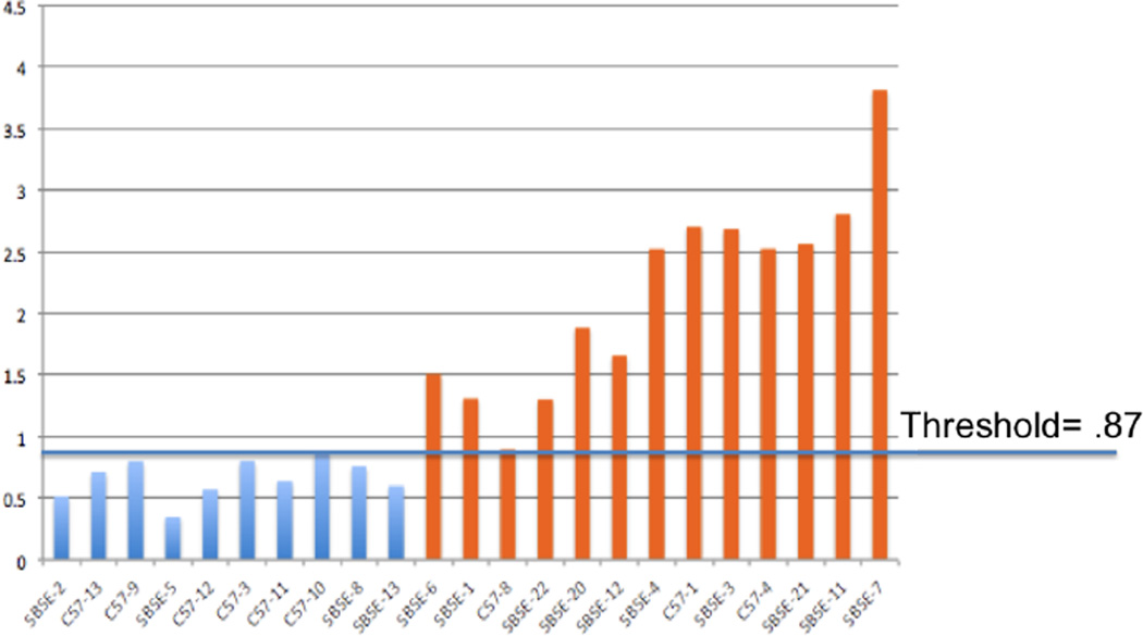
To provide ground truth for the global symmetry score, an expert divided the mandible pairs into two groups, “minimal asymmetry” and “significant asymmetry” (as inidcated by the color of the bars in Fig. 1), then visually ranked each of the 23 mandible pairs in the dataset from most symmetric to least symmetric. This ranking is shown by the order on the X-axis in Fig. 1. We compared the global asymmetry scores of the two groups, indicated by the height of the bars in Fig. 1, and found that they could be separated by a threshold of 0.87. Furthermore, the correlation coefficient between the expert ranking and the global symmetry scores was 0.92.

Fig. 1.

Global symmetry scores for ranked mandibles. Blue indicates minimal asymmetry and orange indicates significant asymmetry. Expert ranking is shown by the order of the X-axis.

B. Local Asymmetry Score Evaluation

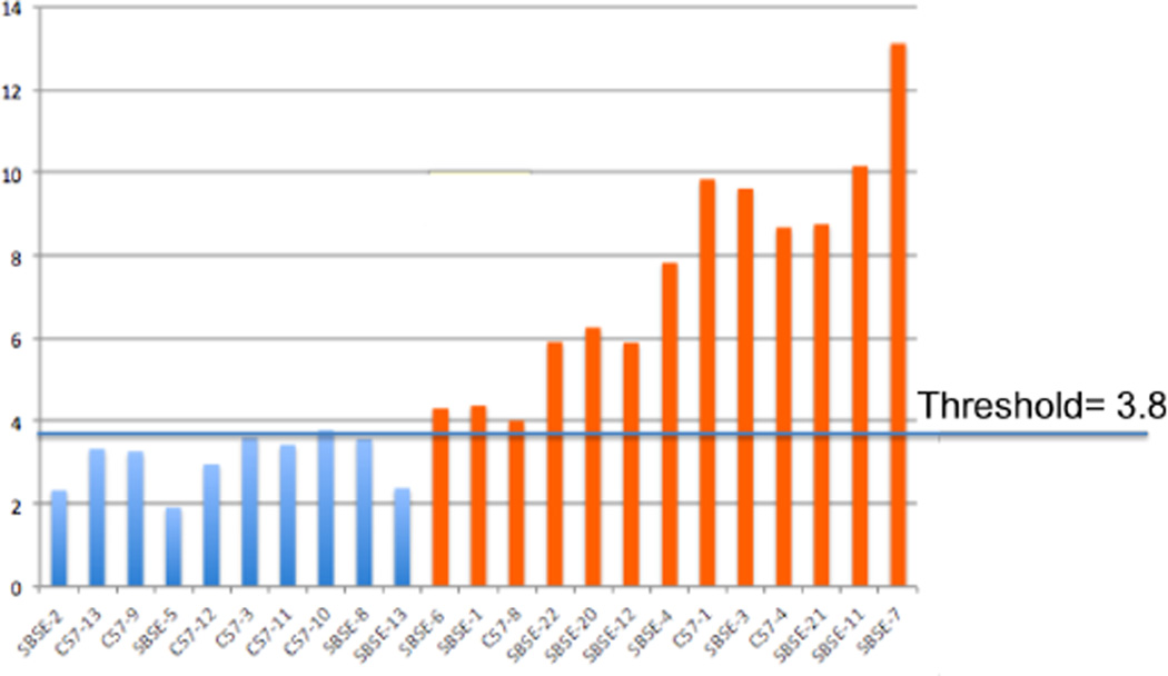
The local symmetry scores were generated using features from connected points around four landmarks identified by an expert. These scores were evaluated using the same method as the global symmetry scores. The “minimal asymmetry” and the “significant asymmetry” groups could be separated using a local symmetry threshold of 3.8. The correlation coefficient between the expert ranking and the global symmetry scores was 0.91 (see Fig. 2).

Fig. 2.

Local symmetry scores for ranked mandibles. Blue indicates minimal asymmetry and orange indicates significant asymmetry. Expert ranking is shown by the order of the X-axis.

C. Similarity of Asymmetry Evaluation

The asymmetry similarity measure provides the distance from each mandible pair in the database to all other mandible pairs, with respect to either deformation magnitude or normal angle difference. Because the similarity measurement uses the spatial distribution of the asymmetry, they are not expected to correspond to the expert rankings in all cases because of the difficulty in incoporating spatial distribution in a simple expert ranking scale. However, in the case of the magnitude asymmetry distances for the most asymmetric pair it would be expected that these would better correspond to the difference in rank. In fact, the correlation coefficient between the expert rankings and distance from the most asymmetric pair is 0.91.

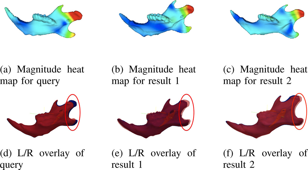
To motivate the usefulness of the magnitude and normal angle difference asymmetry measures, two sample queries are shown. In Fig. 3 a sample query is shown for the magnitude clusters, using the cluster center and average magnitude features. The query image chosen is the most asymmetric case: Fig. 3(a). In the left/right overlay in Fig. 3(d), the left hemi-mandible, shown in blue, is clearly longer than the right hemi-mandible, shown in red. The top two matches for magnitude of asymmetry are also shown in Figures 3(b) and 3(c). Both show a similar magnitude of asymmetry in the condyloid and angular processes. These regions are also circled in Figures 3(d), 3(e), and 3(f). Note that in the “result” images, the left mandible is shorter than the right. This is expected since the direction of the asymmetry is ignored and only the magnitude of the flow vectors is considered. This type of query can be used to find mandibles with asymmetries similar in magnitude but independent of direction.

Fig. 3.

Heat maps and left/right overlay from a sample magnitude query using the most asymmetric mandible. In the top row the high magnitude is represented by red and the low by blue. In the lower row the right hemi-mandible is shown in blue and the left in red.

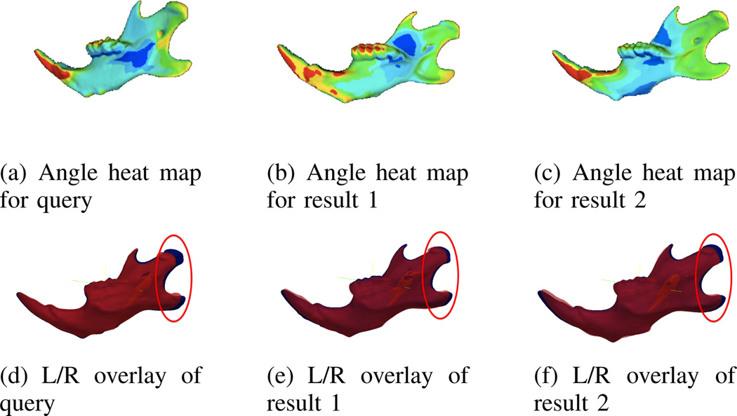
In Fig. 4, the sample query is shown for the normal angle clusters, using the cluster center and average normal angle difference features. The query image is the same as in the previous example and the top two matches for normal angle asymmetry are shown, but notably are different to those identified by the magnitude query. Compared to the magnitude query results, the difference is much smaller for the result images when using these features as a query. For this example, in both matches, the left hemi-mandible is shorter than the right like the query mandible. This type of query can be used to find asymmetries which are similar in direction despite differences in magnitude.

Fig. 4.

Heat maps and left/right overlay from a normal angle difference query using the most asymmetric mandible. In the top row the largest normal angle difference is represented by red and the lowest by blue. In the lower row the right hemi-mandible is shown in blue and the left in red.

VI. CONCLUSION AND FUTURE WORK

In this paper, a new tool is introduced and shown to be capable of assigning asymmetry scores based on global features and features from user-defined locations. Regions of significant asymmetry are detected, described, and used to quantify the similarity of asymmetry across individuals. These methods were evaluated on mouse mandibles with varying amounts of asymmetry and the results are summarized in Table I. Planned future work will create an online user interface to flexibly use and combine the methods provided by this tool. This will allow the tool to be easily accessed by multiple researchers to quantify and characterize the asymmetry of any bilaterally paired structure.

TABLE I.

Summary of Asymmetry Scoring Results

Method	Correlation to Expert Ranking
Global Asymmetry Score	0.92
Local Asymmetry Score	0.91
Magnitude similarity to most asymmetric case	0.91

References

- 1.Combes B, Prima S. New algorithms to map asymmetries of 3d surfaces. Medical Image Computing and Computer-Assisted Intervention–MICCAI 2008. 2008:17–25. doi: 10.1007/978-3-540-85988-8_3. [DOI] [PubMed] [Google Scholar]
- 2.Crum WR, Hartkens T, Hill DLG. Non-rigid image registration: theory and practice. British journal of radiology. 2004;77(Special Issue 2):S140. doi: 10.1259/bjr/25329214. [DOI] [PubMed] [Google Scholar]
- 3.Darvann TA, Hermann NV, Larsen P, Ólafsdóttir H, Hansen IV, Hove HD, Christensen L, Rueckert D, Kreiborg S. Biomedical Imaging: From Nano to Macro, 2010 IEEE International Symposium on. IEEE; 2010. Automated quantification and analysis of mandibular asymmetry; pp. 416–419. [Google Scholar]
- 4.Lancaster JL, Kochunov PV, Thompson PM, Toga AW, Fox PT. Asymmetry of the brain surface from deformation field analysis. Human brain mapping. 2003;19(2):79–89. doi: 10.1002/hbm.10105. [DOI] [PMC free article] [PubMed] [Google Scholar]
- 5.Olafsdottir H, Lanche S, Darvann TA, Hermann NV, Larsen R, Ersboll BK, Oubel E, Frangi AF, Larsen P, Perlyn CA, et al. Proceedings of the 10th international conference on Medical image computing and computer-assisted intervention. Springer-Verlag; 2007. A point-wise quantification of asymmetry using deformation fields: application to the study of the crouzon mouse model; pp. 452–459. [DOI] [PubMed] [Google Scholar]
- 6.Rolfe SM, Shapiro LG, Cox TC, Maga AM, Cox LL. Engineering in Medicine and Biology Society, EMBC 2011 Annual International Conference of the IEEE. IEEE; 2011. A landmark-free framework for the detection and description of shape differences in embryos; pp. 5153–5156. [DOI] [PMC free article] [PubMed] [Google Scholar]