Susceptibility-Weighted Imaging: Technical Aspects and Clinical Applications, Part 1

Abstract

SUMMARY: Susceptibility-weighted imaging (SWI) is a new neuroimaging technique, which uses tissue magnetic susceptibility differences to generate a unique contrast, different from that of spin density, T1, T2, and T2*. In this review (the first of 2 parts), we present the technical background for SWI. We discuss the concept of gradient-echo images and how we can measure local changes in susceptibility. Armed with this material, we introduce the steps required to transform the original magnitude and phase images into SWI data. The use of SWI filtered phase as a means to visualize and potentially quantify iron in the brain is presented. Advice for the correct interpretation of SWI data is discussed, and a set of recommended sequence parameters for different field strengths is given.

Susceptibility-weighted imaging (SWI) is a new means to enhance contrast in MR imaging.^1–56 Until recently, with the exception of phase being used for large-vessel flow quantification or for use in inversion recovery sequences, most diagnostic MR imaging relied only on the reading of magnitude information. The phase information was ignored and usually discarded before even reaching the viewing console. Phase images, however, contain a wealth of information about local susceptibility changes between tissues,^{1,22,26,57–63} which can be useful in measuring iron content²⁶ and other substances that change the local field. The effects of other background magnetic fields presented a major problem by obscuring the useful phase information. Hence, for nearly 20 years, phase information in flow-compensated sequences went essentially unused as a means to measure susceptibility in clinical MR imaging.

In 1997, we developed a means to remove most of the unwanted phase artifacts and keep just the local phase of interest.¹ This set the stage for discovering other aspects of susceptibility imaging and even hinted at the future direction of susceptibility mapping.²⁶ We began to see different types of contrast in the SWI filtered phase images for different diseases. To make the information more accessible to radiologists, though phase and magnitude images separately are also critical pieces of information, we combined the phase and the magnitude information and thus created a new susceptibility-weighted magnitude image, which today is referred to as SWI.²² This new pair of images (the SWI filtered phase data and the merged SWI magnitude data) is now available on at least 1 major manufacturer's systems (Siemens Medical Systems), though it took almost 10 years to see the actual implementation of this approach in a clinical setting around the world.

Many technical developments take years to leave the research environment and become part of standard radiology applications. This has been true for perfusion imaging, diffusion tensor imaging, magnetization transfer imaging, and also for SWI. The common feature of these methods is that they originated as good scientific ideas; they were simulated at first and then tested on phantoms, on volunteers, and finally on a few patients with the appropriate institutional review board approvals from the local institution where the research took place. These methods became scientifically adopted on a larger scale once they showed how clinically capable they were. If successful, the National Institutes of Health would grant funds for broader testing of these methods. Finally, with proof of the value of the method in place and with a stable software package, it would be possible for hundreds of institutions to begin using these methods for diagnostic purposes. However, even then, the final goal will not have been achieved. The method would still need to be adopted in a broad clinical environment and then executed as a standard “neuroprotocol” on a clinical platform. Once the latter step has taken place, the method should eventually be adopted by the radiology community as a whole and become part and parcel of conventional educational courses offered at radiology meetings for accreditation. Only then could we say that a method is fully incorporated into the international radiology routine.

In this review, we summarize the motivation behind SWI, the concepts that led to its discovery, the optimal parameters to use, and the interpretation of the SWI processed data and phase images; and we conclude by discussing the technology in use today, the postprocessing, and future directions of SWI research.

MR imaging has already an overabundance of different approaches for investigational anatomic, functional, and metabolic imaging. Each method focuses on a new issue, such as the delivery of blood to the tissue in perfusion-weighted imaging or molecular motion along a fiber track in diffusion tensor imaging. The susceptibility information is an adjunct to what is available with conventional spin density, T1-, and T2-weighted imaging methods. SWI offers information about any tissue that has a different susceptibility than its surrounding structures such as deoxygenated blood, hemosiderin, ferritin, and calcium. There are numerous neurologic disorders that can benefit dramatically from a very sensitive method that monitors the amount of iron in the brain, whether in the form of deoxyhemoglobin, ferritin, or hemosiderin. Such diseases and conditions include, but are not limited to, aging, multiple sclerosis (MS), stroke, trauma, vascular malformations, and tumors. There is no doubt that as SWI becomes more broadly accepted, we will see many new applications develop because of the astute observations of clinical researchers and the wide availability of information for the whole spectrum of neurologic diseases seen on a daily basis in the clinical setting.

Gradient-Echo Imaging

Historically, data were first collected with a free induction decay.^64,65 The concept of a spin-echo was invented only when it was seen that local field inhomogeneities had caused dramatic signal intensity loss. For some time, the spin-echo approach was the mainstay of clinical MR imaging for resistive machines.⁶⁶ Not long after the appearance of superconducting systems on the market, gradient-echo imaging^67–69 came back to life because the field uniformity in these systems was markedly better (and has continued to improve during the last 20 years). People quickly realized that they could eliminate most artifacts in magnitude images by running the gradient-echo scans with short TEs in sequences like magnetization-preparation rapid acquisition of gradient echo.⁷⁰ This high-bandwidth sequence had little distortion and offered excellent T1 contrast (and presented a good method to collect T1-weighted data even at 3T). Longer TEs were used in 2D gradient-echo imaging but with fairly thick sections, usually 3 or 4 mm. The TEs were often chosen to be 15, 20, or rarely 25 ms because of the signal-intensity loss associated with rapid phase changes across a voxel. Imaging with longer TEs, while maintaining image quality, was only possible with 3D gradient-echo imaging. Once this was recognized and resolutions on the order of ≤1 mm³ were realized with a sufficient signal intensity–to-noise ratio (SNR), the ability to look at hidden information in phase data became possible.^57,71 Thus, the stage to study susceptibility effects was set in the mid 1990s, and the first article on SWI was published in 1997.¹ To appreciate the basic elements of SWI, we must first review the basic gradient-echo sequence design on which it is based.

In MR imaging, it is necessary to create some transverse magnetization first.⁷² This can be accomplished by using a transmit coil to produce a radio-frequency (rf) pulse which tips the longitudinal magnetization (M_o) partially or completely into the transverse plane. The rf pulse is applied at the Larmor frequency, ω = γB_o. If M_o is rotated an angle θ about the x-axis, it will create a component along y that will be picked up by a receiver coil. The data are then encoded in both the phase- and partition-encoding directions (y and z, respectively, for a transverse acquisition), while a dephasing gradient is applied in the readout direction. The read gradient is then turned on and the data are sampled. After this, the remnant signal intensity is further dephased, and rf spoiling is applied by varying the axis about which the rf is applied so that no transverse magnetization remains before the next rf pulse. All this is shown pictorially in Fig 1. The magnitude signal-intensity response for this rf-spoiled short-TR gradient-echo sequence is given by

(1)

where ρ_o is the tissue spin density, TR is the repeat time of each data acquisition, T1 is the tissue longitudinal relaxation time, and θ is the angle by which the magnetization is tipped (usually called the flip angle). A signal-intensity behavior example is given for white matter, gray matter, and CSF for 1.5T and 3T (Fig 2 and Table 1). The full signal-intensity response is given by (for a right-handed system)

(2)

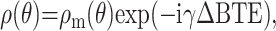
where ΔB represents the local field deviation caused by iron, for example, and γ is the gyromagnetic constant, which is equal to 2π · 42.58 MHz/T for protons. This can be rewritten as

(3)

where g is a geometric factor, Δχ is the difference of the local magnetic susceptibility of the tissue of interest from its surroundings, and B₀ is the field strength. Starting with the Larmor equation

(4)

the expression for phase is

(5)

Fig 1.

Gradient-echo sequence design. T_s refers to the sampling time interval. The gradient pulses are designed to give first-order flow compensation. SS indicates the slice-select gradient; PE, the phase-encoding gradient; ADC, analog-to-digital conversion.

Fig 2.

A, Plots showing the signal-intensity behavior as a function of flip angle for gray matter (GM) and white matter (WM) at field strengths 1.5T and 3T. B, Plots showing the corresponding contrast between GM-WM and GM-CSF. These curves are calculated taking into consideration the higher signal intensity available at 3T and assuming that bandwidth is correspondingly increased at 3T to ensure equivalent geometric distortion. Tissue parameters are given in Table 1. Note that the GM/WM contrast is highest around 20° at 3T and there is a minimum or reversal of contrast around 5° (where GM is now brighter than WM; ie, it is a high-contrast spin echo-weighted image).

Table 1:

Tissue parameters used to simulate the T1-weighted images shown in Fig 2

	GM	WM	CSF
Spin density %	80	65	100
1.5T	1000 ms	650 ms	4000 ms
3T	1283 ms	838 ms	4000 ms

Note:—GM indicates gray matter; WM, white matter; CSF, cerebrospinal fluid. CSF is taken to have 100% water content.

The change in phase between 2 tissues after a period of time, TE, can then be written as

where

so that

(6)

(7)

All of ΔB, Δχ, and, therefore, Δφ are dependent on the local tissue susceptibility.

Magnetic Susceptibility

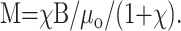
Magnetic susceptibility is defined as the magnetic response of a substance when it is placed in an external magnetic field. When an object is placed inside a uniform magnetic field, the induced magnetization, M, is given by

(8)

where

(9)

and χ is the magnetic susceptibility relating M and H. We can also write

(10)

where μ = μ_oμ_r is the permeability, μ_o is the permeability in vacuum, μ_r is the relative permeability, and H the magnetic field (B is the induced magnetic field). Using the relative permeability as

(11)

we find

(12)

For linear materials with χ ≪ 1, we find

(13)

and it becomes clear that the induced magnetization is directly proportional to the main field and the magnetic susceptibility. Each tissue or substance behaves somewhat differently in a magnetic field. For the purposes of this review, we shall consider only diamagnetic and paramagnetic substances. Diamagnetic substances have χ < 0. For example, calcium in the body tends to be in the form of calcium phosphates such as Ca₃(PO)₄ and is diamagnetic. On the other hand, paramagnetic substances (ie, most iron-based materials or tissues) have χ > 0. For example, deoxygenated blood has Δχ ≈ 0.45 ppm in SI units, relative to surrounding tissue. Moreover, iron-containing proteins, like ferritin and hemosiderin, tend to have varying susceptibilities depending on the amount of sequestered iron within the protein. Typically, on the basis of phase measurements from 75 subjects,⁶² approximately a Δχ = 0.21 ppm in SI units with respect to CSF, corresponds to 60 μg of iron (Fe) per gram of tissue (although this may underestimate the amount of Fe by a factor of 5). The susceptibilities of most biologic tissues⁷³ tend to be <10⁻⁴. However, all forms of iron may not be visible with MR imaging if Δχ = 0 for that substance. This can happen if the iron is shielded by other elements such as oxygen. For a more detailed description of the different forms of magnetism see Schenck⁷³ and Saini et al.⁷⁴

Geometry Effects

The induced magnetization (owing to its susceptibility) in an object within a uniform external magnetic field distorts the uniform field outside the object. The spatial distribution of this deviation in the external applied field is a function of the geometry of the object.⁷⁵ The local field deviation inside and around an object is of interest because it gives rise to local phase differences in MR imaging. When discussing the effects of geometry on local field variations, we usually neglect the background field and assume that χ ≪ 1. For a cylinder making an angle θ to the main field, the effect on the field inside the cylinder is given by

(14)

which includes the Lorentzian sphere term. We have used Δχ = χ_i − χ_e. Here, χ_i and χ_e are the susceptibilities inside and outside the cylinder, respectively. Generally, when we are looking at changes in local tissue fields, the final term χ_eB_o / 3 no longer plays a role because it is a common constant both inside and outside the object. If we write

(15)

we have

(16)

For blood vessels in particular, we have

(17)

where

(18)

Here, A is a constant to be determined by the absolute susceptibility of blood in vivo, Hct is the hematocrit, and Y is the oxygen saturation. Practically, the choice of A depends on the value of Y in vivo: with A = 1, then Y = 0.55,¹ whereas with A = 1.5, then Y = 0.70.^76,77

The field outside is more complicated and is given by

(19)

where a is the radius of the blood vessel, which is assumed as a long cylinder intercepting an angle θ with the main field, r is the distance perpendicularly from the axis of the cylinder to the position, and Φ is the angle between the vector r and the projection of the main field direction onto a plane perpendicular to the axis of the vessel. The constant term, χ_eB_o / 3, has been dropped in equation 19.

For more complicated structures, the expressions for magnetic field variations around the object are not so straightforward. The key point is that susceptibility differences between 2 adjacent structures lead to a spatial field deviation within and around them, which is a function of their geometries. Following equation 6, this field deviation in turn leads to local phase changes in the MR phase images. However, phase images contain information about all magnetic fields, microscopic and macroscopic. The former may be from small amounts of local iron deposits, for example, whereas the latter consists of field changes caused by the geometry of the object, such as air/tissue interface effects, and by inhomogeneities in the main magnetic field. With all these properties brought together, the phase should be written as

(20)

All these terms are a function of the spatial location. The first term contains the local field changes of interest. The second term represents a chemical shift effect and causes changes of the form

(21)

where σ represents the chemical shift. The difference between chemical shift and the first term in equation 20 is that chemical shift has no geometry dependence but is more of a point field change.⁷⁵ The last 2 terms create artifacts and are not our interest. They tend to have a low spatial-frequency dependence (the phase varies slowly over the image) and, for this reason, can be removed with a high-pass (HP) filter.⁶⁰

Creating Susceptibility-Weighted Filtered-Phase Images

First, an HP filter is applied to remove the low-spatial frequency components of the background field. This is usually done by using a 64 × 64 low-pass filter divided into the original phase image (eg, an image with a matrix size of 512 × 512) to create an HP-filter effect. The end result is the HP filter. Specifically, the HP-filtered image is obtained by taking the original image ρ(r), truncating it to the central n × n complex image ρ_n(r), creating an image by zero-filling the elements outside the central n × n elements, and then complex dividing ρ(r) by ρ_n(r) to obtain a new image,⁶⁰

(22)

which has most of the bothersome parts of the terms ΔB_{global geometry} + ΔB_{main field} removed (Fig 3).

Fig 3.

A, Raw phase image. B, HP-filtered phase image with a central filter size of 32 × 32; C, Filtered-phase image with a central filter size of 64 × 64.

Once we have a pristine phase image with the background field changes removed, the door is open to differentiate one type of tissue from another, depending on their susceptibilities. This may be particularly useful at high field because the T1 difference between tissues begins to decrease, but any changes in susceptibility remain the same. Figure 4 shows an example of a T1-weighted image compared with the gradient-echo magnitude and phase data. Here we see that the gray matter, especially in the motor cortex area—the central sulcus—is clearly delineated in the phase image because of its iron content. Figure 5 shows an example of a phase image in the midbrain.

Fig 4.

Short-echo T1-weighted image (A), compared with the SWI long-echo gradient-echo processed magnitude (B) and HP-filtered phase data (C).

Fig 5.

A, HP-filtered phase image in the midbrain acquired at 4T with TE = 15 ms. B, India ink-stained cadaver brain section showing a strong correspondence to variations in signal intensity as seen with SWI HP-filtered phase.

Marrying Magnitude and Phase Images to Create Magnitude SWI Data

Although HP-filtered phase images themselves are quite illustrative of the susceptibility contrast, they are influenced by both the intratissue phase (from ΔB_in) and the associated extratissue phase (from ΔB_out), which can impair the differentiation of adjacent tissues with different susceptibilities. Hence, the “phase mask” is designed to enhance the contrast in the original magnitude image by suppressing pixels having certain phase values. Magnitude and phase data are brought together as a final magnitude SWI dataset by multiplying a phase mask image into the original magnitude image.²²

The phase mask is designed to be a number between zero and 1. When there are no phase characteristics that we want to enhance, the phase mask is set to 1. Otherwise, the phase mask is designed to suppress the signal intensity in areas where the phase takes on certain values. For example, if the phase of interest is negative, the mask is designed as

(23)

where φ(x) is the phase at location x. The phase mask can be applied any number of times to the original magnitude image ρ(x) to create a new image,

(24)

with a different contrast. The number of phase mask multiplications is chosen to optimize the contrast-to-noise ratio of the SWI image. This mathematical masking process is illustrated in Fig 6 and with a specific example from a 1.5T dataset shown in Fig 7.

Fig 6.

Pictorial depiction of the phase-masking process. A, Phase profile in a filtered-phase image. B, Corresponding profile of the mask created from A. Once the mask is raised to the fourth power, the vein that has a phase of −π / 2 and a mask value of 0.5 will become 1-/16 and, therefore, this vein will be almost as well suppressed as the vein with a phase of −π and f(x) = 0. GM indicates gray matter; WM, white matter.

Fig 7.

A, Unprocessed original SWI magnitude image. B, HP-filtered phase image. C, Processed SWI magnitude image (ie, after phase-mask multiplication with m = 4). D, Unprocessed original SWI magnitude image showing the dark hypointense ring around vein cross-sections (arrows). E, HP-filtered phase image showing the veins have low signal-intensity (arrows). F, Processed SWI magnitude image showing that the veins now appear with uniform low signal intensity (arrows).

A simple mathematical model can be built to estimate the value of m (from Equation 24).³⁰ The number of multiplications needed for a phase ≥0.3π is ≤4. For a phase <0.3π, a value of m ≥ 4 should be used. However, choosing m = 4 for a phase of 0.1π or π causes <25% reduction in visibility in either case, suggesting that m = 4 is a good compromise if one is limited to just 1 representative SWI dataset. Of course, m can be varied to produce a series of SWI data that can be used in a diagnosis. After this processing, the data are often viewed by using a minimum intensity projection (mIP) over ≥4 images. Clinically, 4 sections are the current common display, though showing a projection over 10 sections can be useful to visualize a larger coverage of the venous drainage system in a given area. Figure 8 shows projection data over the original magnitude images and the SWI processed images. One can also present the data as a sliding mIP, which means that one starts with the original series of images and mIPs over 4, moves to the next original image and mIP over 4 again so that a series of 64 images now becomes a series of 61 mIP images.

Fig 8.

mIP data over the original magnitude images (A) and over the processed SWI images (B). The mIP is carried out over 7 sections (representing a 14-mm slab thickness). The images were collected at 3T. There is a dropout of signal intensity in the frontal part of the brain, but otherwise the vessel visibility is much improved in B. In the future, this frontal dropout should not be a problem when the air/tissue geometries are corrected (Fig 9).

Furthermore, combining phase and magnitude information ensures the detectability of signal-intensity changes coming from both T2 and susceptibility differences between tissues. The existence of a phase difference does not necessarily lead to a T2* effect (uniform phase causes no T2′ decay), so these 2 sources of information complement each other. Also, suppressing the veins fully helps to create a clear distinction between veins and arteries (Fig 7D−F). Therefore, we see that both magnitude and phase information are essential for proper tissue characterization, hence their marriage to create an SWI processed image.

Advanced Phase Processing

The HP-filtering method described earlier is quite successful in removing the spatially slowly varying phase effects that obscure the local intertissue phase differences of interest. However, apart from removing the spatially slowly varying background field effects, the HP filter (depending on filter size) also removes some of the physiologically or pathophysiologically relevant phase information from larger anatomic structures. For this reason, it is rare to use a central filter larger than 64 × 64 if one is interested in measuring iron content. If the main goal is just to create better MR venograms, then it is reasonable to use a central filter of 96 × 96 or 128 × 128 without much adverse effect on the small vessels.

The larger the filter size, the more background field effects can be removed, but also the concomitant loss of phase information from larger tissue structures is more probable. Ideally, background field effects could be removed by predicting the phase expected for a given individual's global head geometry. This would leave only small low-spatial-frequency phase errors, allowing a smaller filter size to be used to create the final HP result.⁷⁸ An example of this novel approach is shown in Fig 9. Although this currently is a time-consuming process, it would not be surprising to see this method implemented in a practical fashion in the coming years, making SWI more robust to air/tissue interface field effects. In that case, it may be possible to tackle problems such as subarachnoid hemorrhages, subdural hemorrhages, and possibly spine imaging.

Fig 9.

Results of the improved processing methodology. A, Original SWI phase image. B, Simulated phase due to air/tissue geometry at 40 ms. C, Result of subtracting A from B through the complex division. D, Result of HP filtering of A. E, Result of HP filtering of C. F, Corresponding unprocessed magnitude SWI image. G, Processed SWI magnitude image by using a phase mask from D. H, Processed SWI magnitude by using a phase mask from E. I, Result of subtracting G from H. Corresponding magnitude and phase images have been adjusted to the same, but appropriate, contrast levels. The size of the central filter in the HP process is 64 × 64.

Another important consideration is measuring iron. Currently, phase, measured from filtered MR images, is found to be the most sensitive tool for measuring relative changes in iron content in the subcortical structures of the brain.⁶² Measuring iron content depends on the assignment of a given phase change in a tissue to a known amount of iron in that tissue. In Haacke et al,⁶² this was done by associating the phase change in the motor cortex with 60 μg of nonheme Fe/g tissue. This ignores the fact that some of the phase shift, if not most of it, may come from heme iron and not ferritin. If this is indeed the case, the same phase shift seen in globus pallidus minus any heme iron effect may have a slope 5 times smaller. In any case, the reader needs to be aware that the absolute relationship between changes in phase and iron has not yet been established and that the relative contributions between heme and nonheme iron have not been sorted out yet. On the other hand, if blood levels remain constant and ferritin concentration does change, then any relative values of iron change in percentages would still be accurate, independent of whether this scale factor of 5 is present or not.

One problem in trying to compare phase information from 1 person to another is the geometry dependence of the phase coming from the shape of local objects of interest. If one assumes that the geometries of the structures of interest are roughly the same from person to person, then this might not be a major concern, but it is a potential problem when trying to measure absolute iron content. (It is less likely to be a problem when measuring relative changes in iron or calcium content.) The susceptibility of a structure is independent of the orientation, size, and shape of the structure; hence, a means to quantify tissue susceptibility would be of utmost importance because it will be a reliable measure of iron content. Tissue susceptibility will be an important means to quantify iron and is a topic of considerable interest in the field today.^26,27

Recommended Imaging Parameters at Different Field Strengths

SWI can be used best at higher field strengths for a number of reasons. First, at low fields, TEs need to be much longer. For example, to obtain optimum contrast for veins at 1.5T, one needs a TE of between 40 and 80 ms. If we try to keep the product ΔχB_oTE constant so that the phase effect remains the same from 1 field strength to another, then the minimum TE at 3T becomes only 20 ms. This can be expressed mathematically as

(25)

which is tantamount to forcing

(26)

where B₀TE and B₀′TE′ refer to the products of field strength and TE at 1.5T and 3T, respectively. This shorter TE has several advantages. First, the scanning at 3T can be run twice as fast compared with 1.5T such that in the same period of time, twice the number of sections can be obtained at 3T or an isotropic in-plane resolution can be obtained. Second, at high fields, the SNR increases, so a sacrifice of some SNR (because the image quality at 1.5T is already good enough clinically) to obtain not only faster coverage but also higher resolution of the whole brain coverage at 3T can be easily tolerated. With parallel imaging at 3T, whole-brain coverage by using SWI can be obtained in as short as 4 minutes. Figure 10 shows the phase behavior as a function of field strength, given that equation 25 is obeyed. As expected, it is difficult to differentiate field strengths except for the fact that the SNR is higher for the 3T image than the 1.5T image. Otherwise, the phase images should have the same contrast.

Fig 10.

A and B, Phase images, keeping the product B_oTE constant. A phase image acquired at 1.5T (A) and the same subject at 3T (B) show the same overall contrast but with a better SNR. The gray/white matter contrast in these images comes from the increased MR-visible iron content in the gray matter, giving it an appearance similar to a T1-weighted scan.

The advent of very high fields such as 7T and above offers unprecedented resolution and SNR in imaging the brain. However, there are concerns about field homogeneity and high specific absorption rates (SAR). Gradient-echo imaging is one of the most robust sequences in MR imaging and continues to show its advantages at high field where images appear much more uniform than spin-echo images. SWI, for example, uses flip angles much smaller than 90°, and because the SAR varies as the square of the flip angles, SWI has a much smaller power deposition than spin-echo sequences. As discussed previously, phase can be kept invariant as a function of field strength by appropriately adjusting the TE. On the other hand, phase information from local structures does not strongly depend on local rf inhomogeneities. These 2 properties suggest that the SWI filtered-phase images can play a role in comparing subject data across field strengths. High-field images are shown in Figs 11 and 12 (for recommended imaging parameters at different field strengths, see Table 2). From the perspective of higher SNR, smaller changes in phase now become visible, and we are beginning to discover new phase variations that reveal venules and arcuate fibers similar to what one sees in stained cadaver brain studies.

Fig 11.

A sample mIP from 7T data, with a resolution of 215 × 215 × 1000 μ, TE = 16 ms, TR = 45 ms, FA = 25°, and mIP over 8 sections. Image courtesy of Ge Y and Barnes S.

Fig 12.

A zoomed image from the same dataset shown in Fig 11 reveals a dark band between the gray matter and white matter, which we assume represents the white matter arcuate fibers (diagonal arrows). The small vessels joining the pial veins are the venules (vertical arrows). Image courtesy of Ge Y and Barnes S.

Table 2:

Range of experimental parameters advised for SWI data collection at different field strengths^*

FS	FA (degrees)	TR (ms)	TE (ms)	BW/pixel (Hz/pixel)
1.5T	18–25 (20)	50–60 (60)	40	70–100
3T	12–17 (12)	25–35 (30)	20	80–100
4T	8–15 (12)	25–35 (28)	15	80–120
7T	11–17 (14)	25–35 (30)	10–16	100–150

Note:—FS indicates field strength; FA, flip angle; BW, bandwidth.

^*The values given in parentheses for FA and TR are the ones generally used by the authors. TEs given here are optimized for maximum signal cancellation from venous vasculature. Slightly shorter or longer TEs can be used for appropriate applications. However, note that for implementing shorter TEs, higher BW would be required, which would adversely affect the SNR of the image. One way to avoid this is to reduce the TR appropriately and cover more sections of the brain, which can recover some of the lost SNR.

Interpreting SWI Data

There are 3 components to interpret in the SWI data to make a clinical diagnosis. The first relates to the original magnitude image from, for example, a TE = 40 ms scan at 1.5T. This image usually will have a resolution of no less than 0.5 (read) × 1.0 (phase) × 2.0 mm (section). Despite the fact that the TE is so long, the image quality will be quite good apart from dephasing around the sinuses and in the air/tissue interface regions such as the pituitary gland. When compared with conventional gradient-echo scans with a TE of 25 ms (where the effects of veins are much less), SWI will tend to highlight small changes in susceptibility across a voxel as signal-intensity losses.

There are 2 key points to keep in mind when interpreting the magnitude data. First, there is no large blooming effect because the resolution is so high. The higher the resolution, the less the blooming artifacts. Second, the parameters of the sequence are chosen so that the contrast is fairly flat between normal gray matter, white matter, and CSF, though a low-enough flip angle can keep the CSF brighter than the surrounding gray and white matter. Consequently, the magnitude image clearly reveals areas with either short T2* or an oscillatory signal intensity in the magnitude image caused by the presence of deoxyhemoglobin in the major veins. This latter effect will cause a much larger signal-intensity loss than the actual T2* of the tissue because the signal intensity from the vein can cancel the signal intensity from the gray matter or white matter and, like water/fat cancellation, will cause a complete loss of signal intensity at the appropriate TE (this is why the TE in SWI was chosen to be 40 ms in the first place). For a vein of subvoxel size, this cancellation leads to a hypointense voxel with respect to its surroundings. However, for a vein covering more than a few voxels, only in those voxels in which both vein and surrounding tissue are partial-volumed do we see these signal-intensity cancellations and hypointense voxels. A voxel containing only the intravenous signal intensity does not show this signal-intensity cancellation effect. Hence, the vein appears to have a bright signal intensity inside with a hypointense ring around it (Fig 7D). Nevertheless, following phase-mask multiplication, the whole vein appears as a hypointense region in the processed SWI image (Fig 7F).

The second component to interpret in SWI data is the phase image. For a right-handed system, veins will look dark on the phase image (because the deoxygenated blood is paramagnetic relative to its surrounding tissue) and calcium will look bright (because calcium is diamagnetic relative to the brain tissue). Remnant phase artifacts may also appear by the air/tissue interfaces and above the sinuses, necessitating a careful recognition of the dark shadows in the phase images in these areas as artifacts. Newer methods are making this less of a problem.^53,78,79 Interpreting a darkening in local areas in phase images is important for MS, where iron can be associated with gray matter and white matter lesions. These iron-laden lesions will often correlate with the MS lesions seen on T2 or fluid-attenuated inversion recovery (FLAIR), but sometimes they will not, presumably depending on the stage and type of lesion.⁸⁰ The phase difference can also be used to quantify iron or follow changes in iron deposition with time, to follow the resolution of cerebral hemorrhages in patients with trauma, or to monitor the development of microbleeds in patients with dementia. In the future, phase will likely also be used to quantify oxygen saturation in major veins. Because the original phase data have been filtered, we often refer to the new phase images as the SWI-filtered phase images.

The third component used in interpreting SWI is the final processed SWI. These data have taken full advantage of T2* signal-intensity losses in the magnitude image and iron increases in the phase images to highlight both types of contrast in a single image. At this point, these images show many “black holes,” most often representing the cross-sections of small veins. How can we discriminate between these cross-sections and microbleeds? The best way to check for vessel connectivity is to take an mIP over a number of sections (most often 4). This is similar to using a maximum intensity projection (MIP) to see arteries in MR angiography (MRA). A point of interest here is that the MIP of SWI data can be taken as well. The resulting image, which is simply an SWI version of an MRA, is not so impressive at 1.5T; but at 3T, this MRA begins to approach the quality of a conventional MRA.⁵³

A key point of practical interest is the orientation used for SWI. This is invariably transverse for a number of reasons. The foremost reason is that the phase of veins perpendicular to the main field is, in theory, opposite to that of those parallel to the main field, with the latter showing a negative phase and the former, a positive phase (equation 17). However, with an in-plane resolution to section-thickness aspect ratio of 2:4, the phase outside the small veins contributes more than the phase inside, reversing the phase behavior so that all veins show a negative phase.³⁰ This reversal of phase behavior makes the processing much easier because only a single negative phase mask needs to be used in the transverse orientation and this makes the visualization of the veins in the SWI-processed images much sharper.

Finally, we consider the contrast in the SWI data. Generally, the low flip angles and intermediate TEs give SWI an odd mixture of contrast. The gray matter/white matter contrast is almost nonexistent. Choosing the flip angle can play a role in getting the CSF signal intensity close to the gray matter/white matter signal intensity. This concept makes the magnitude images of little utility except as markers for microhemorrhages or other susceptibility effects. We often choose a slightly higher flip angle that suppresses partially the CSF, making it slightly darker than gray matter or white matter and (similar to FLAIR) slightly T1-weighted. In that case, edema appears bright, whereas the CSF remains suppressed. For patients with tumor, this has the effect of showing both the peritumoral edema as well as the bleeding inside the tumor.

Conversely, choosing a lower flip angle tends to highlight the spin attenuation and makes CSF a bit brighter than gray matter or white matter to regain some contrast. The former choice of, for example, 20° at 1.5T is the most popular. After processing, the SWI takes advantage of the high iron content in gray matter and begins to recreate gray matter/white matter contrast. The phase image has a lot of resemblance to a T1-weighted image. This gets carried over to the SWI. At the end, to better delineate the nature of the vascular content, we perform an MIP of the SWIs, usually over 4 adjacent images, to create an effective 8-mm-thick section. These mIP images present a great tool for visualizing vessel connectivity and microbleed locations with respect to the vasculature and other structures in the brain.

Future Directions

To date, SWI has had most of its clinical applications in the neuroimaging arena (this will be covered in Part 2 to be published in a later issue).⁸¹ Many of the ideas relating to iron quantification remain to be validated in animal models and further tested longitudinally in patients. Technical developments such as creating susceptibility maps that remove all phase artifacts are a particularly exciting direction.^78,82 This would open the door to being able to use SWI in the spine, for example. Other developing applications include imaging cartilage, imaging calcium in atherosclerosis, imaging breast, and liver hemochromatosis.

References

- 1.Reichenbach JR, Venkatesan R, Schillinger DJ, et al. Small vessels in the human brain: MR venography with deoxyhemoglobin as an intrinsic contrast agent. Radiology 1997;204:272–77 [DOI] [PubMed] [Google Scholar]
- 2.Baudendistel KT, Reichenbach JR, Metzner R, et al. Comparison of functional MR-venography and EPI-BOLD fMRI at 1.5 T. Magn Reson Imaging 1998;16:989–91 [DOI] [PubMed] [Google Scholar]
- 3.Reichenbach JR, Essig M, Haacke EM, et al. High-resolution venography of the brain using magnetic resonance imaging. MAGMA 1998;6:62–69 [DOI] [PubMed] [Google Scholar]
- 4.Essig M, Reichenbach JR, Schad LR, et al. High-resolution MR venography of cerebral arteriovenous malformations. Magn Reson Imaging 1999;17:1417–25 [DOI] [PubMed] [Google Scholar]
- 5.Lee BC, Kuppusamy K, Grueneich R, et al. Hemispheric language dominance in children demonstrated by functional magnetic resonance imaging. J Child Neurol 1999;14:78–82 [DOI] [PubMed] [Google Scholar]
- 6.Lin W, Mukherjee P, An H, et al. Improving high-resolution MR bold venographic imaging using a T1 reducing contrast agent. J Magn Reson Imaging 1999;10:118–23 [DOI] [PMC free article] [PubMed] [Google Scholar]
- 7.Tan IL, van Schijndel RA, Pouwels PJ, et al. MR venography of multiple sclerosis. AJNR Am J Neuroradiol 2000;21:1039–42 [PMC free article] [PubMed] [Google Scholar]
- 8.Reichenbach JR, Barth M, Haacke EM, et al. High-resolution MR venography at 3.0 Tesla. J Comput Assist Tomogr 2000;24:949–57 [DOI] [PubMed] [Google Scholar]
- 9.Cheng YC, Haacke EM. Predicting BOLD signal changes as a function of blood volume fraction and resolution. NMR Biomed 2001;14:468–77 [DOI] [PubMed] [Google Scholar]
- 10.Cheng YC, Haacke EM, Yu YJ. An exact form for the magnetic field density of states for a dipole. Magn Reson Imaging 2001;19:1017–23 [DOI] [PubMed] [Google Scholar]
- 11.Schad LR. Improved target volume characterization in stereotactic treatment planning of brain lesions by using high-resolution BOLD MR-venography. NMR Biomed 2001;14:478–83 [DOI] [PubMed] [Google Scholar]
- 12.Reichenbach JR, Haacke EM. High-resolution BOLD venographic imaging; a window into brain function. NMR Biomed 2001;14:453–67 [DOI] [PubMed] [Google Scholar]
- 13.Reichenbach JR, Jonetz-Mentzel L, Fitzek C, et al. High-resolution blood oxygen-level dependent MR venography (HRBV): a new technique. Neuroradiology 2001;43:364–69 [DOI] [PubMed] [Google Scholar]
- 14.Essig M, Reichenbach JR, Schad L, et al. High resolution MR-venography of cerebral arteriovenous malformations [in German]. Radiologe 2001;41:288–95 [DOI] [PubMed] [Google Scholar]
- 15.Haacke EM, Herigault G, Yu Y, et al. Observing tumor vascularity noninvasively using magnetic resonance imaging. Image Analysis and Stereology 2002;21:107–13 [Google Scholar]
- 16.Tong KA, Ashwal S, Holshouser BA, et al. Hemorrhagic shearing lesions in children and adolescents with posttraumatic diffuse axonal injury: improved detection and initial results. Radiology 2003;227:332–39 [DOI] [PubMed] [Google Scholar]
- 17.Essig M, Waschkies M, Wenz F, et al. Assessment of brain metastases with dynamic susceptibility-weighted contrast-enhanced MR imaging: initial results. Radiology 2003;228:193–99 [DOI] [PubMed] [Google Scholar]
- 18.Abduljalil AM, Schmalbrock P, Novak V, et al. Enhanced gray and white matter contrast of phase susceptibility-weighted images in ultra-high-field magnetic resonance imaging. J Magn Reson Imaging 2003;18:284–90 [DOI] [PubMed] [Google Scholar]
- 19.Hermier M, Nighoghossian N. Contribution of susceptibility-weighted imaging to acute stroke assessment. Stroke 2004;35:1989–94 [DOI] [PubMed] [Google Scholar]
- 20.Wycliffe ND, Choe J, Holshouser B, et al. Reliability in detection of hemorrhage in acute stroke by a new three-dimensional gradient recalled echo susceptibility-weighted imaging technique compared to computed tomography: a retrospective study. J Magn Reson Imaging 2004;20:372–77 [DOI] [PubMed] [Google Scholar]
- 21.Tong KA, Ashwal S, Holshouser BA, et al. Diffuse axonal injury in children: clinical correlation with hemorrhagic lesions. Ann Neurol 2004;56:36–50 [DOI] [PubMed] [Google Scholar]
- 22.Haacke EM, Xu Y, Cheng YC, et al. Susceptibility weighted imaging (SWI). Magn Reson Med 2004;52:612–18 [DOI] [PubMed] [Google Scholar]
- 23.Haddar D, Haacke E, Sehgal V, et al. Susceptibility weighted imaging: theory and applications. J Radiol 2004;85:1901–08 [DOI] [PubMed] [Google Scholar]
- 24.Rauscher A, Sedlacik J, Barth M, et al. Noninvasive assessment of vascular architecture and function during modulated blood oxygenation using susceptibility weighted magnetic resonance imaging. Magn Reson Med 2005;54:87–95 [DOI] [PubMed] [Google Scholar]
- 25.Sehgal V, Delproposto Z, Haacke EM, et al. Clinical applications of neuroimaging with susceptibility-weighted imaging. J Magn Reson Imaging 2005;22:439–50 [DOI] [PubMed] [Google Scholar]
- 26.Haacke EM, Cheng NY, House MJ, et al. Imaging iron stores in the brain using magnetic resonance imaging. Magn Reson Imaging 2005;23:1–25 [DOI] [PubMed] [Google Scholar]
- 27.Mentzel HJ, Dieckmann A, Fitzek C, et al. Early diagnosis of cerebral involvement in Sturge-Weber syndrome using high-resolution BOLD MR venography. Pediatr Radiol 2005;35:85–90 [DOI] [PubMed] [Google Scholar]
- 28.Babikian T, Freier MC, Tong KA, et al. Susceptibility weighted imaging: neuropsychologic outcome and pediatric head injury. Pediatr Neurol 2005;33:184–94 [DOI] [PubMed] [Google Scholar]
- 29.Rauscher A, Sedlacik J, Barth M, et al. Magnetic susceptibility-weighted MR phase imaging of the human brain. AJNR Am J Neuroradiol 2005;26:736–42 [PMC free article] [PubMed] [Google Scholar]
- 30.Xu Y, Haacke EM. The role of voxel aspect ratio in determining apparent vascular phase behavior in susceptibility weighted imaging. Magn Reson Imaging 2006;24:155–60 [DOI] [PubMed] [Google Scholar]
- 31.Hamans BC, Barth M, Leenders WP, et al. Contrast enhanced susceptibility weighted imaging (CE-SWI) of the mouse brain using ultrasmall superparamagnetic iron oxide particles (USPIO). Z Med Phys 2006;16:269–74 [DOI] [PubMed] [Google Scholar]
- 32.Sehgal V, Delproposto Z, Haddar D, et al. Susceptibility-weighted imaging to visualize blood products and improve tumor contrast in the study of brain masses. J Magn Reson Imaging 2006;24:41–51 [DOI] [PubMed] [Google Scholar]
- 33.Haacke EM. Susceptibility weighted imaging (SWI). Z Med Phys 2006;16:237. [DOI] [PubMed] [Google Scholar]
- 34.Ashwal S, Babikian T, Gardner-Nichols J, et al. Susceptibility-weighted imaging and proton magnetic resonance spectroscopy in assessment of outcome after pediatric traumatic brain injury. Arch Phys Med Rehabil 2006;87:S50–58 [DOI] [PubMed] [Google Scholar]
- 35.Yoshida Y, Terae S, Kudo K, et al. Capillary telangiectasia of the brain stem diagnosed by susceptibility-weighted imaging. J Comput Assist Tomogr 2006;30:980–82 [DOI] [PubMed] [Google Scholar]
- 36.Noebauer-Huhmann IM, Pinker K, Barth M, et al. Contrast-enhanced, high-resolution, susceptibility-weighted magnetic resonance imaging of the brain: dose-dependent optimization at 3 Tesla and 1.5 Tesla in healthy volunteers. Invest Radiol 2006;41:249–55 [DOI] [PubMed] [Google Scholar]
- 37.Haacke EM, DelProposto ZS, Chaturvedi S, et al. Imaging cerebral amyloid angiopathy with susceptibility-weighted imaging. AJNR Am J Neuroradiol 2007;28:316–17 [PMC free article] [PubMed] [Google Scholar]
- 38.Vinod Desai S, Bindu PS, Ravishankar S, et al. Relaxation and susceptibility MRI characteristics in Hallervorden-Spatz syndrome. J Magn Reson Imaging 2007;25:715–20 [DOI] [PubMed] [Google Scholar]
- 39.Akter M, Hirai T, Hiai Y, et al. Detection of hemorrhagic hypointense foci in the brain on susceptibility-weighted imaging clinical and phantom studies. Acad Radiol 2007;14:1011–19 [DOI] [PubMed] [Google Scholar]
- 40.Larsen JP, Britt WI, Kido D, et al. Susceptibility weighted magnetic resonance imaging in the evaluation of dementia. Radiology Case Reports 2007;2:102. [DOI] [PMC free article] [PubMed] [Google Scholar]
- 41.Sedlacik J, Rauscher A, Reichenbach JR. Obtaining blood oxygenation levels from MR signal behavior in the presence of single venous vessels. Magn Reson Med 2007;58:1035–44 [DOI] [PubMed] [Google Scholar]
- 42.Pinker K, Noebauer-Huhmann IM, Stavrou I, et al. High-resolution contrast-enhanced, susceptibility-weighted MR imaging at 3T in patients with brain tumors: correlation with positron-emission tomography and histopathologic findings. AJNR Am J Neuroradiol 2007;28:1280–86 [DOI] [PMC free article] [PubMed] [Google Scholar]
- 43.Shen Y, Kou Z, Kreipke CW, et al. In vivo measurement of tissue damage, oxygen saturation changes and blood flow changes after experimental traumatic brain injury in rats using susceptibility weighted imaging. Magn Reson Imaging 2007;25:219–27 [DOI] [PubMed] [Google Scholar]
- 44.Ohta A, Naito K, Ohkubo M, et al. Study of susceptibility-weighted imaging (SWI) using a simple MR phantom [in Japanese]. Nippon Hoshasen Gijutsu Gakkai Zasshi 2007;63:1093–98 [DOI] [PubMed] [Google Scholar]
- 45.Thomas B, Somasundaram S, Thamburaj K, et al. Clinical applications of susceptibility weighted MR imaging of the brain: a pictorial review. Neuroradiology 2008;50:105–16 [DOI] [PubMed] [Google Scholar]
- 46.de Souza JM, Domingues RC, Cruz LC, et al. Susceptibility-weighted imaging for the evaluation of patients with familial cerebral cavernous malformations; a comparison with T2-weighted fast spin-echo and gradient-echo sequences. AJNR Am J Neuroradiol 2008;29:154–58 [DOI] [PMC free article] [PubMed] [Google Scholar]
- 47.Harder SL, Hopp KM, Ward H, et al. Mineralization of the deep gray matter with age: a retrospective review with susceptibility-weighted MR imaging. AJNR Am J Neuroradiol 2008;29:176–83 [DOI] [PMC free article] [PubMed] [Google Scholar]
- 48.Sedlacik J, Helm K, Rauscher A, et al. Investigations on the effect of caffeine on cerebral venous vessel contrast by using susceptibility-weighted imaging (SWI) at 1.5, 3 and 7 T. Neuroimage 2008;40:11–18 [DOI] [PubMed] [Google Scholar]
- 49.Somasundaram S, Kesavadas C, Thomas B. Susceptibility weighted imaging in holohemispheric venous angioma with cerebral hemiatrophy. Neurol India 2008;56:104–05 [DOI] [PubMed] [Google Scholar]
- 50.Liu HL, Wai YY, Chen WS, et al. Hemorrhage detection during focused-ultrasound induced blood-brain-barrier opening by using susceptibility-weighted magnetic resonance imaging. Ultrasound Med Biol 2008;34:598–606 [DOI] [PubMed] [Google Scholar]
- 51.Koopmans PJ, Manniesing R, Niessen WJ, et al. MR venography of the human brain using susceptibility weighted imaging at very high field strength. MAGMA 2008;21:149–58. Epub 2008 Jan 11 [DOI] [PubMed] [Google Scholar]
- 52.Fushimi Y, Miki Y, Togashi K, et al. A developmental venous anomaly presenting atypical findings on susceptibility-weighted imaging. AJNR Am J Neuroradiol 2008;29:E56. [DOI] [PMC free article] [PubMed] [Google Scholar]
- 53.Du YP, Jin Z. Simultaneous acquisition of MR angiography and venography (MRAV). Magn Reson Med 2008;59:954–58 [DOI] [PubMed] [Google Scholar]
- 54.Hammond KE, Lupo JM, Xu D, et al. Development of a robust method for generating 7.0 T multichannel phase images of the brain with application to normal volunteers and patients with neurological diseases. Neuroimage 2008;39:1682–92 [DOI] [PMC free article] [PubMed] [Google Scholar]
- 55.Zhong K, Leupold J, von Elverfeldt D, et al. The molecular basis for gray and white matter contrast in phase imaging. Neuroimage 2008;40:1561–66 [DOI] [PubMed] [Google Scholar]
- 56.Hu J, Yu Y, Juhasz C, et al. MR susceptibility weighted imaging (SWI) complements conventional contrast enhanced T1 weighted MRI in characterizing brain abnormalities of Sturge-Weber syndrome. J Magn Reson Imaging 2008;28:300–07 [DOI] [PMC free article] [PubMed] [Google Scholar]
- 57.Haacke EM, Lai S, Yablonskiy DA, et al. In-vivo validation of the BOLD mechanism: a review of signal changes in gradient-echo functional MRI in the presence of flow. International Journal of Imaging Systems and Technology 1995;6:153–63 [Google Scholar]
- 58.Haacke EM, Lai S, Reichenbach JR, et al. In vivo measurement of blood oxygen saturation using magnetic resonance imaging: a direct validation of the blood oxygen level-dependent concept in functional brain imaging. Human Brain Mapp 1997;5:341–46 [DOI] [PubMed] [Google Scholar]
- 59.Akbudak E, Norberg RE, Conturo TE. Contrast-agent phase effects: an experimental system for analysis of susceptibility, concentration, and bolus input function kinetics. Magn Reson Med 1997;38:990–1002 [DOI] [PubMed] [Google Scholar]
- 60.Wang Y, Yu Y, Li D, et al. Artery and vein separation using susceptibility-dependent phase in contrast-enhanced MRA. J Magn Reson Imaging 2000;12:661–70 [DOI] [PubMed] [Google Scholar]
- 61.Fernandez-Seara MA, Techawiboonwong A, Detre JA, et al. MR susceptometry for measuring global brain oxygen extraction. Magn Reson Med 2006;55:967–73 [DOI] [PubMed] [Google Scholar]
- 62.Haacke EM, Ayaz M, Khan A, et al. Establishing a baseline phase behavior in magnetic resonance imaging to determine normal vs. abnormal iron content in the brain. J Magn Reson Imaging 2007;26:256–64 [DOI] [PubMed] [Google Scholar]
- 63.Duyn JH, van Gelderen P, Li TQ, et al. High-field MRI of brain cortical substructure based on signal phase. Proc Natl Acad Sci U S A 2007;104:11796–801 [DOI] [PMC free article] [PubMed] [Google Scholar]
- 64.Young IR, Bailes DR, Burl M, et al. Initial clinical evaluation of a whole body nuclear magnetic resonance (NMR) tomograph. J Comput Assist Tomogr 1982;6:1–18 [DOI] [PubMed] [Google Scholar]
- 65.Bydder GM, Steiner RE. NMR imaging of the brain. Neuroradiology 1982;23:231–40 [DOI] [PubMed] [Google Scholar]
- 66.Bailes DR, Young IR, Thomas DJ, et al. NMR imaging of the brain using spin-echo sequences. Clin Radiol 1982;33:395–414 [DOI] [PubMed] [Google Scholar]
- 67.Edelstein WA, Hutchison JM, Johnson G, et al. Spin warp NMR imaging and applications to human whole-body imaging. Phys Med Biol 1980;25:751–56 [DOI] [PubMed] [Google Scholar]
- 68.Haase A, Frahm J, Matthaei D, et al. Flash imaging: rapid NMR imaging using low flip-angle pulses. J Magn Reson 1986;67:258–66 [DOI] [PubMed] [Google Scholar]
- 69.Frahm J, Haase A, Matthaei D. Rapid 3-dimensional MR imaging using the flash technique. J Comput Assist Tomogr 1986;10:363–68 [DOI] [PubMed] [Google Scholar]
- 70.Mugler JP 3rd, Brookeman JR. Three-dimensional magnetization-prepared rapid gradient-echo imaging (3D MP RAGE). Magn Reson Med 1990;15:152–57 [DOI] [PubMed] [Google Scholar]
- 71.Reichenbach JR, Venkatesan R, Yablonskiy DA, et al. Theory and application of static field inhomogeneity effects in gradient-echo imaging. J Magn Reson Imaging 1997;7:266–79 [DOI] [PubMed] [Google Scholar]
- 72.Haacke EM, Brown R, Thompson M, et al. Magnetic Resonance Imaging: Physical Principles and Sequence Design. New York: Wiley;1999. :5
- 73.Schenck JF. The role of magnetic susceptibility in magnetic resonance imaging: MRI magnetic compatibility of the first and second kinds. Med Phys 1996;23:815–50 [DOI] [PubMed] [Google Scholar]
- 74.Saini S, Frankel RB, Stark DD, et al. Magnetism: a primer and review. AJR Am J Roentgenol 1988;150:735–43 [DOI] [PubMed] [Google Scholar]
- 75.Chu SC, Xu Y, Balschi JA, et al. Bulk magnetic susceptibility shifts in NMR studies of compartmentalized samples: use of paramagnetic reagents. Magn Reson Med 1990;13:239–62 [DOI] [PubMed] [Google Scholar]
- 76.Weisskoff RM, Kiihne S. MRI susceptometry: image-based measurement of absolute susceptibility of MR contrast agents and human blood. Magn Reson Med 1992;24:375–83 [DOI] [PubMed] [Google Scholar]
- 77.Spees WM, Yablonskiy DA, Oswood MC, et al. Water proton MR properties of human blood at 1.5 Tesla: magnetic susceptibility, T(1), T(2), T*(2), and non-Lorentzian signal behavior. Magn Reson Med 2001;45:533–42 [DOI] [PubMed] [Google Scholar]
- 78.Neelavalli J, Cheng YC, Haacke EM. Removal of Air/Tissue Interface Field Effects in Susceptibility Weighted Imaging. Proceedings of International Society of Magnetic Resonance in Medicine. Toronto, Ontario, Canada; 3–9 May2008. . Abstract 3499
- 79.Rauscher A, Barth M, Reichenbach JR, et al. Automated unwrapping of MR phase images applied to BOLD MR-venography at 3 Tesla. J Magn Reson Imaging 2003;18:175–80 [DOI] [PubMed] [Google Scholar]
- 80.Haacke EM, Makki M, Ge Y, et al. Characterizing iron deposition in multiple sclerosis lesions using susceptibility weighted imaging. J Magn Reson Imaging 2009. (In press). [DOI] [PMC free article] [PubMed]
- 81.Tong KA, Ashwal S, Obenaus A, et al. Susceptibility-weighted MR imaging: a review of clinical applications in children. AJNR Am J Neuroradiol 2008;29:9–17 [DOI] [PMC free article] [PubMed] [Google Scholar]
- 82.de Rochefort L, Brown R, Prince MR, Wang Y. Quantitative MR susceptibility mapping using piece-wise constant regularized inversion of the magnetic field. Magn Reson Med 2008;60:1003–09 [DOI] [PubMed] [Google Scholar]