Abstract
One key problem in computational neuroscience and neural engineering is the identification and modeling of functional connectivity in the brain using spike train data. To reduce model complexity, alleviate overfitting, and thus facilitate model interpretation, sparse representation and estimation of functional connectivity is needed. Sparsities include global sparsity, which captures the sparse connectivities between neurons, and local sparsity, which reflects the active temporal ranges of the input-output dynamical interactions. In this paper, we formulate a generalized functional additive model (GFAM) and develop the associated penalized likelihood estimation methods for such a modeling problem. A GFAM consists of a set of basis functions convolving the input signals, and a link function generating the firing probability of the output neuron from the summation of the convolutions weighted by the sought model coefficients. Model sparsities are achieved by using various penalized likelihood estimations and basis functions. Specifically, we introduce two variations of the GFAM using a global basis (e.g., Laguerre basis) and group LASSO estimation, and a local basis (e.g., B-spline basis) and group bridge estimation, respectively. We further develop an optimization method based on quadratic approximation of the likelihood function for the estimation of these models. Simulation and experimental results show that both group-LASSO-Laguerre and group-bridge-B-spline can capture faithfully the global sparsities, while the latter can replicate accurately and simultaneously both global and local sparsities. The sparse models outperform the full models estimated with the standard maximum likelihood method in out-of-sample predictions.
Keywords: functional connectivity, generalized linear model, sparsity, penalized likelihood, basis function, spike trains, temporal coding
1. Introduction
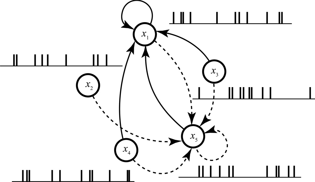
One key problem in computational neuroscience and neural engineering is the identification of functional connectivity in the brain (Okatan et al. 2005; Stevenson et al. 2009; Eldawlatly et al. 2009; Brown et al. 2004; Reed and Kaas 2010; Pillow et al. 2008). Functional connectivity, in the context of ensemble unitary neural recording, refers to the causal relations in spiking activities of a population of neurons (Fig. 1). Identification of the neural functional connectivity is a necessary step towards understanding how neurons in a brain region are organized to represent, transmit, process information, and further perform higher cognitive functions. Due to its quantitative and predictive nature, it also serves as the computational basis for the development of cortical neural prostheses (Berger et al. 2005; Berger et al. 2010; Song et al. 2007, 2009a; Berger et al. 2011).
Figure 1.
Schematic diagram showing the functional connectivity within a neuron population. For a given neuron (#1), the functional connectivity is defined as the causal relations (solid arrowed lines) between the spike trains (x1, x2, x3, x4, and x5) of all neurons to the spike train of this neuron (x1). This procedure is repeated for other neurons (e.g., dashed arrowed lines for neuron #5) to derive the functional connectivity of the whole population.
Neural functional connectivity can be studied with various computational and mathematical techniques motivated by different theoretical frameworks. Commonly used approaches can be classified into the following non-mutually exclusive categories: generalized linear model (Eldawlatly et al. 2009; Okatan et al. 2005; Truccolo et al. 2005; Paninski et al. 2004; Zhao et al. 2012; Chen et al. 2011), Volterra-type systems identification (Song et al. 2007, 2009a; Zanos et al. 2008), Granger causality (Kim et al. 2011; Nedungadi et al. 2009), and information theory, e.g., mutual information (Lin et al. 2012; Paninski 2003), directed information (Quinn et al. 2011; So et al. 2012) and transfer entropy (Garofalo et al. 2009; Gourevitch and Eggermont 2007; Ito et al. 2011). In systems identification, which is the main approach of this study, the identification problem is equivalent to the nonlinear dynamical modeling of the input-output properties of neural ensembles (Song and Berger 2009).
To identify or model the neural functional connectivity, several essential characteristics of neurons and their activities need to be taken into account. First, neurons work cooperatively in networks. They typically receive spike train inputs from, and send spike train outputs to, multiple other neurons. The input-output dynamics of a neural ensemble have to be studied within a multi-input, multi-output (MIMO) framework. Second, neurons communicate with each other with spikes. Since axonal spikes have highly similar if not identical waveforms, information is carried in the timings of the spikes (i.e., temporal patterns). The model formulation should reflect the point-process nature of the input/output signals, and thus, respect the temporal code. Third, the activity of an output neuron depends not only on the current activities of other neurons, but also on their past spiking histories. This requires the model to be dynamical. Fourth, the transformation from input spikes to output spikes involves numerous nonlinear processes such as short-term synaptic plasticity (Song et al. 2009b; Song et al. 2009c; Zucker and Regehr 2002), ligand-gated ion channels, dendritic integration, active membrane conductances, spike generation, after-potential, and interneuronal inhibition (Hille 1992; Hines and Carnevale 2000; Johnston 1999). The model needs to be capable of capturing the input-output nonlinearities caused by these neurobiological processes. Last, neurons in the brain tend to be sparsely connected. An output neuron typically is innervated by only a small subset of neurons in its input region and thus exhibits high level of sparsity in space. In addition, given a functional connection, the time span of the effect of an input neuron on the output neuron has a limited range, and thus results in an additional form of sparsity in the temporal domain. Revealing such sparse neural functional connectivity is the main thrust of this study. It is also worthy to note that, in most of the experiments, neurons are highly under-sampled, i.e., only a very small number of neurons can be recorded from a given neuronal population. The synaptic connectivities and the associated nonlinear dynamical biophysical mechanism are typically approximated at the functional level. The under-sampling problem and the associated unobserved common-input problem need to be aware of in interpreting the functional connectivity (Aertsen et al. 1989; Paninski et al. 2004; Pillow et al. 2005; Stevenson et al. 2008; Vidne et al. 2012), e.g., the identified functional connectivity cannot be directly interpreted as synaptic connections.
In this study, we formulate a generalized functional additive model (GFAM) for the identification of the neural functional connectivity. A GFAM extends the generalized linear model (McCullagh and Nelder 1989; Truccolo et al. 2005), which consists of a linear component and a link function, by expanding the unknown input-output transfer functions with a set of basis functions. Adding basis functions takes advantage of the continuity in the unknown function and facilitates the model estimation by reducing the total number of model coefficients. In the context of sparse GFAM (Gerhard et al. 2011; Gerwinn et al. 2010; Harris et al. 2003), we further introduce the concepts of global sparsity and local sparsity, which correspond to the sparsities in the input-output pairs and system memories, and represent them in the model coefficient space as zero values at group level and sub-group level, respectively. Since the standard maximum likelihood method cannot generate sparse estimations, various penalized estimation methods (e.g., LASSO, group LASSO, and group bridge) and bases (e.g., Laguerre basis and B-spline basis) are developed and used to yield different forms of sparse representations of the model. Specifically, the proposed group bridge method can estimate both the global and local sparsity simultaneously.
The paper is organized as the follows. In Section 2, we formally introduce the modeling problem; describe the GFAM framework, global and local bases, and the penalized likelihood estimation methods. In Section 3, we test the GFAMs with different basis functions and penalized likelihood estimations using synthetic data, and then apply the GFAM to the identification of the hippocampal CA3-CA1 functional connectivity using spike trains recorded from rodents performing a memory-dependent behavioral task.
2. Methods
2.1. Dynamical Multi-Input, Single-Output Model
Consider a set of spike trains recorded from a population of neurons (Fig. 1). To identify the functional connectivity of this neuron population, we model the causal relationship H between the spike train recorded from one neuron (i.e., a single output signal denoted by y(t)) and the spike trains recorded from the whole neuron population (i.e., input signals denoted by x1(t), …, xN(t)).
| (1) |
where X(t) = (x1(t), …, xN(t))T, N is the number of input signals, and M is the memory length of the system. Note that X can contain the output signal y itself in order to include the autoregressive effect of the preceding activities of the output neuron, with the lag τ starting from 1 instead of 0 (i.e., 0 < τ ≤ M) for this input. To simplify the notation, this distinction is omitted in our definition above. With a sufficiently small sampling interval (e.g., 2 msec), both x and y only contain binary values, i.e., 1 when there is a spike and 0 when there is no spike.
This definition forms a dynamic, finite-memory, multi-input, single-output (MISO) model of spike trains. The modeling goal is to predict the event (i.e., 1 or 0) observed in the output at time t given all the preceding activities collected from all inputs within the finite memory window. Considering the stochastic nature of spike generation, it can be expressed as modeling the probability of a spike being observed as in:
| (2) |
Note that in this formulation of functional connectivity, only neural spiking activities are considered and the derived model is behavioral task-independent. To include the task-dependence of the functional connectivity, behavioral variables can be added as additional inputs into the model (Harris et al., 2003; Truccolo et al., 2005).
2.2. Generalized Functional Additive Model
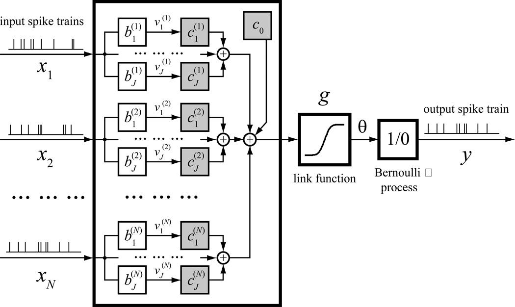
There are many different approaches to solve the above modeling problem. One approach is using a generalized functional additive model (GFAM) as shown in Figure 2:
| (3) |
where k0 is a scalar zeroth-order kernel function, k(n) are first-order kernel functions describing the relationship between the output spike probability and the nth input. For simplicity, we deal with the first-order model in this section. g(·) is a known link function. To model binary output, logit and probit are two commonly used functions. Under the logit link, Equation 3 can be rewritten as
| (4) |
Figure 2.
Structure of a generalized functional additive model (GFAM) of spike trains. In this model, the spike train inputs (x) are convolved with a set of basis functions (b), multiplied with the corresponding coefficients (c), summed, and fed into a link function (g) to form the firing probability intensity (θ). Output spike train y is considered a realization of θ. Note that the output spike train can also be included as an input to model the autoregressive dynamics of the output neuron. The shaded blocks represent the model coefficients to be estimated.
Under the probit link function, Equation 3 can be rewritten as
| (5) |
where erf is the Gaussian error function defined as
| (6) |
We choose to use the probit link function in this study for its convenient neurobiological interpretation as a noisy threshold function that transforms the pre-threshold membrane potential to output spikes (Song et al. 2007, 2009a). However, despite the different physical interpretations, there is only subtle difference between these link functions, e.g., the logistic distribution function has slightly heavier tails than the normal density function (Kutner et al. 2004).
2.3. Functional Expansion with Basis Functions
In Equation 3, each first-order kernel function k(n) contains M + 1 coefficients. The number of coefficients is large when the memory length is long and/or the sampling interval is small. For example, the causal effect of one neuron to another neuron can last for hundreds of milliseconds to seconds. In order to retain the temporal information of spike trains, the sampling interval has to be small enough that each interval contains no more than one spike. It is often in the order of milliseconds (2 msec in this study). This will result in hundreds to thousands of model coefficients to be estimated. On the other hand, real life kernel functions always contain some degree of smoothness; independent estimation of all model coefficients is seldom necessary. Taking advantage of such smoothness, a common way of reducing the number of model coefficients is the functional expansion technique, where the kernel functions are approximated as the weighted summation of a set of predefined basis functions:
| (7) |
where c are the coefficients of the basis functions, b are the basis functions, and J is the number of basis functions. The set of basis functions form a linear space. Any function k(τ), τ ∈[0, M], can be approximated by an element in this space. Such an approximation will be exact if the function k(·) itself belongs to the linear space. Equation 3 then can be rewritten as:
| (8) |
where v are the convolutions of the basis functions and the inputs, c is the vector of model coefficients, ϕ is the concatenation of 1 and v as in
| (9) |
| (10) |
| (11) |
Since J can be made much smaller than M, the number of coefficients to be estimated is greatly reduced. In addition, the functional expansion also separates the system dynamics in the mathematical expression (Marmarelis 2004), i.e., the temporal convolution with inputs appears only in Equation 9; Equation 8 is a static (i.e., instantaneous or memoryless) operation to the convolved values v that does not involve the lag τ. This Wiener-Bose type of expression is mathematically more convenient than its original form in Equation 3, especially in the extension to the nonlinear cases.
2.4. Local and Global Basis Functions
The basis functions can take various forms. A trivial choice is a set of delayed (τ ∈[0, M]) Kronecker delta functions. Using this basis, the original form of the model in Equation 1 is recovered from the Weiner-Bose form as in Equation 8 and 9.
In this paper, we describe and utilize two types of basis functions: local basis and global basis. Local basis is a set of basis functions with local support; that is, each function covers (i.e., has non-zero values in) a local region of the system memory ([0, M]). As a contrast, global basis is a set of basis functions that span (i.e., has no continuous zeroed values in) the entire system memory. For computational efficiency and stability, global basis functions are often designed to be orthonormal.
Polynomial splines are piecewise polynomials with smooth transitions between the adjacent pieces at a set of interior knot points. Specifically, a polynomial spline of degree d ≥ 0 on [0, M] with m > 0 interior knot points and the knot sequence η0 = 0 < η1 < … < ηm < ηm+1 = M is a function that is a polynomial of degree d between each pair of adjacent knots, and has d − 1 continuous derivatives for d ≥ 1. Together with many other groups in statistics and neuroscience (Eilers and Marx 1996; Kass and Ventura 2001; Truccolo and Donoghue 2007), we use B-spline as the local basis in this study for its computational stability (Schumaker 1980; de Boor 1972).
Mathematically, the B-spline basis functions of degree d can be defined in a recursive fashion. In particular, the jth basis function can be expressed using the Cox-de Boor formula
| (12) |
where
| (13) |
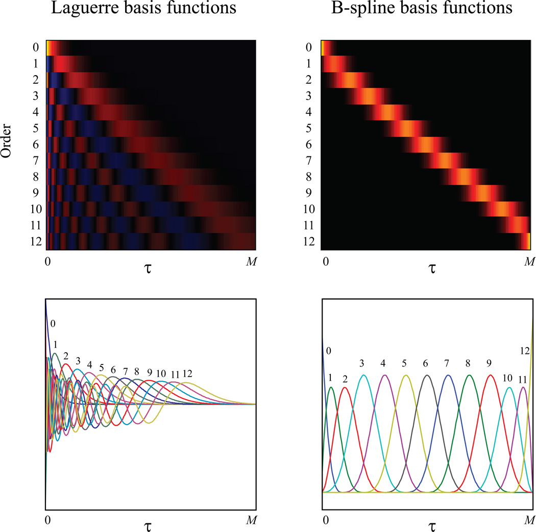
For a given sequence of m knots and a fixed degree d, the total number of B-spline basis functions is J = m+d+1. In Figure 3, a set of cubic (d = 3) B-spline basis functions defined on [0, 500] are plotted. There are m = 9 interior knots evenly distributed on the entire domain, yielding a total of J = 13 basis functions. Throughout this paper, it is assumed without loss of generality that all B-spline basis functions are normalized to integrate to 1.
Figure 3.
Global and local basis functions. Global basis functions (e.g., Laguerre basis functions) expand the entire system memory [0, M], while local basis functions (e.g., B-spline basis functions) cover a local region of the system memory. Left panel: Laguerre basis functions (zeroth to 12th order). Right panel: B-spline basis functions (zeroth to 12th order). Top panel: basis functions in 2D color plots (yellow: positive values; blue: negative values; black: zero values). Bottom panel: basis functions in line plots.
The global basis used in this study is the Laguerre basis function (Marmarelis 1993; Ogura 1972).
The jth order Laguerre basis function Lj can be expressed as
| (14) |
Laguerre basis functions constitute an orthonormal basis. They can be calculated recursively (Marmarelis, 1987, 1993) as
| (15) |
Even more conveniently, v, the convolutions of L and x, also can be calculated recursively (Marmarelis 1993; Ogura 1972) as
| (16) |
Figure 3 shows the first 13 Laguerre basis functions. It is evident that all L expand the entire system memory [0, M]. Laguerre parameter α controls the rate of exponential decay of the basis functions. The larger α is, the slower L decay.
Note that basis functions are typically defined as starting from the zeroth order, so J basis functions means [b0, b1, … bJ−1]. However, to simplify notation, we will use [b1, b2, … bJ] to represent the same set of basis in places other than this section.
2.5. Maximum Likelihood Estimation of the Generalized Functional Additive Model
The GFAM defined in Equation 8 and 9 can be estimated using the traditional maximum likelihood method. Assuming that the elements of y are conditionally independent given the present and past of the input signals [X(t − τ), 0 ≤ τ ≤ M], the joint likelihood of the observation can be written as
| (17) |
The log-likelihood is
| (18) |
Plugging the basis functions as in Equation 9 to approximate θ(t) in the above equation yields an approximation of l. This new criterion is a function of basis function coefficients c = (c(1), … , c(N))’ and denoted by l(c), where c(n) = (c(n)(1), c(n)(2), … , c(n)(J))’. The maximizer of l(c) is the maximum likelihood estimator (MLE) that is denoted by ĉmle.
Since v can be calculated from b and x, Equation 6 constitutes a generalized linear model where y is the dependent variable, v are the independent variables, and c are the sought model coefficients. Functional model coefficient c can be estimated with the standard iterative reweighted least-squares method to obtain ĉmle (McCullagh and Nelder 1989). By plugging ĉmle into Equation 7, kernel functions k0 and k are reconstructed with the basis functions (k0 is simply equal to c0). However, these estimators would not normally have zero values. Therefore, they will not achieve the desired model sparsity; or in other words, the model complexity will not be reduced using the maximum likelihood estimation.
2.6. Global Sparsity and Local Sparsity
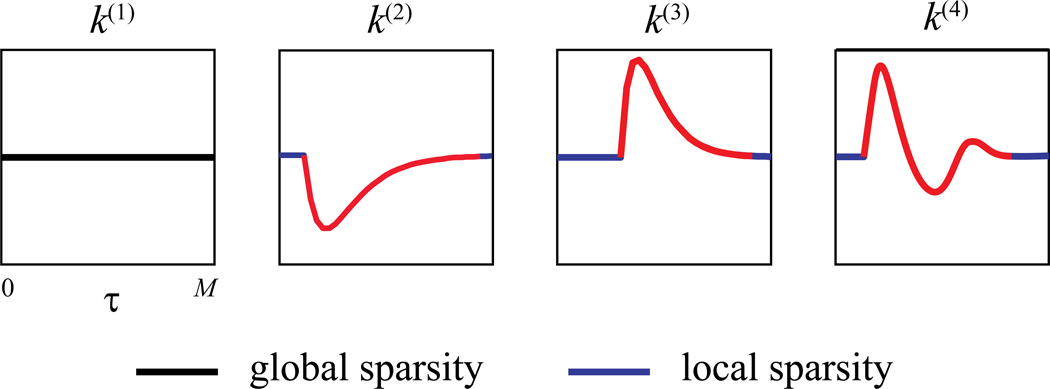
In this section, we introduce the concepts of two forms of sparsities in the context of neural functional connectivity (Tu et al. 2012). One is global sparsity, which refers to the sparsity of model coefficients at the group level. In a GFAM, model coefficients are naturally grouped with respect to the inputs with which they are associated, i.e., [k(n)(τ), 0 ≤ τ ≤ M] all belong to the nth input and thus are within the same group. Given this grouping setting, global sparsity then refers to the occurrence that kernel functions for some inputs remain zero-valued over the entire system memory (i.e., 0 ≤ τ ≤ M). The other is local sparsity, which refers to the sparsity of model coefficients within groups. In a GFAM, given the above grouping setting, local sparsity means that the kernel functions may take zero values over a continuous period within the system memory.
Figure 4 gives an illustrative example of global and local sparsities. The zero-valued coefficients corresponding to the global sparsity are plotted in black, while the zero-valued coefficients corresponding to the local sparsity are plotted in blue.
Figure 4.
Global sparsity and local sparsity of functional connectivity. Global sparsity refers to the occurrence that kernel functions k for some inputs remain zero-valued over the entire system memory, e.g., k(1). Local sparsity means that the kernel functions may take zero values over a continuous period of time within the system memory, e.g., blue regions in k(2), k(3), and k(4).
2.7. Composite-Penalty for Sparse GFAMs
In this section, we further describe a composite-penalized likelihood method for the estimation of sparse representations of GFAMs.
First, we consider the consequences of using basis functions for the estimation of sparse GFAMs. As defined previously, global basis functions expand the entire system memory without continuous zeroed values. Therefore, a GFAM using global basis functions can achieve only global sparsity when all coefficients belonging to a certain group are equal to zero. Local sparsity normally cannot be obtained when a subset of these coefficients are equal to zero. By contrast, local basis functions cover a local region of the system memory. Consequently, a GFAM using local basis functions can achieve both global sparsity when all coefficients belonging to a certain group are equal to zero, and local sparsity when a subset of these coefficients are equal to zero. The problem then becomes how to select and estimate model coefficients (1) at a group level for the global basis, and (2) at both group and subgroup levels for the local basis.
Now we describe the penalized estimation methods. One common approach is grouping the model coefficients c, taking ‖·‖β norm over them, and adding γ power over the norm. Moreover, based on the different sizes (cardinalities) of the groups, constant weights can be added. Specifically, the composite penalty P for coefficients c is defined as
| (19) |
where gi are subscripts of subsets of c according to a grouping method (see below). Scalars a are constants to adjust the weights of each coefficient group. They can be chosen naturally as a proportion to the size of the gi. G is the total number of groups.
Using the grouping structure defined by the inputs, Equation 19 can be rewritten as
| (20) |
where a is omitted given that each group contains the same number of coefficients.
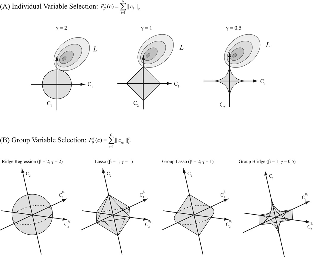
Some widely used penalty functions are special cases of Equation 20. For example, when β = 1 (i.e., taking |·| norm), γ = 1, and a = 1, there is essentially no grouping structure and Equation 20 is equivalent to the LASSO penalty (Tibshirani 1996; Chen et al. 2011; Zhao et al. 2012; Kelly et al. 2010) as shown in Figure 5
| (21) |
Figure 5.
Schematic diagram of penalty functions for individual-variable and group-variable estimations and selections. A: individual-variable shrinkage and selections. B: group-variable shrinkage and selections.
It has been proven that LASSO can achieve individual coefficient selection. Using global basis functions, neither global sparsity nor local sparsity is guaranteed; using local basis functions, only local sparsity is guaranteed.
If we group the coefficients c according to the kernel functions of inputs without overlap, and let β = 2, γ = 1, Equation 20 becomes the group LASSO penalty term (Yuan and Lin 2006)
| (22) |
The group LASSO penalty can be considered as a hybrid of L2-penalty and L1-penalty. Within the groups, it shrinks (but does not select) the coefficients with the L2-norm regularization (i.e., ridge regression); across groups, it selects the groups in a L1-norm regularization (i.e., LASSO) fashion (Fig. 5). Using this penalty, coefficients can be selected at the group level but not the sub-group level. In other words, this penalty can achieve global sparsity but not local sparsity. In this study, we will use the , i.e., group LASSO, and global basis to estimate GFAMs with only global sparsity. Group LASSO method has been used in a previous study with a raised cosine basis (Pillow et al. 2008).
Let β = 1, γ < 1, then Equation 20 becomes the group bridge penalty (Huang et al. 2009), under which both individual and group variable selection can be achieved. The group bridge penalty can be considered as a hybrid of L1-penalty and Lγ-penalty, i.e., bridge penalty (Frank and Friedman 1993). Within groups, it selects the coefficients with the L1-norm regularization (i.e., LASSO); across groups, it selects with Lγ regularization (i.e., bridge regression; Fig. 5). Naturally, we will use the , i.e., group bridge, and local basis to estimate GFAMs with both global and local sparsities. Specifically in the case of using B-spline basis, the value of kernel function on each segment between two adjacent knots only depends on a local set of B-spline basis functions. Thus, we can group the coefficients according to this property, and use the .
The penalty can be written as
| (23) |
For simplicity and numerical stability, we choose γ = 0.5 for computation in this study. Ideally, γ can be optimized using a cross-validation procedure. After being constructed in this way, the penalty can achieve both global and local sparsities of the kernel functions.
2.8. Estimation of the Sparse GFAMs
In this paper, instead of using the log-likelihood function, we choose to directly work with the negative log-likelihood function. In particular, the composite penalized (negative) log-likelihood criterion (objective function) can be written as
| (24) |
where λ ≥ 0 is a tuning parameter that controls the relative importance of the likelihood and the penalty term. When λ takes on a larger value, the estimation yields sparser result of the coefficients. The estimates of model coefficients can be obtained by minimizing the penalized log-likelihood criterion as
| (25) |
Note that the optimization problem is rather challenging since both components in Equation 24, the negative log-likelihood function and the penalty function, may not be convex. Here, we take two steps to treat each component respectively.
First, we obtain the maximum likelihood estimator ĉmle using the standard iteratively reweighted least-squares method for generalized linear models (McCullagh and Nelder 1989). Moreover, ĉmle is then used as the initial value of c to approximate locally the likelihood function l(c) as
| (26) |
The second term could be omitted since ∇l(ĉmle) = 0. Using such quadratic approximation of the log-likelihood function, we have
| (27) |
For logit link function, straightforward computation shows that ∇2l(ĉmle) = −ΦT RΦ, where
For probit link function, the expression of ∇2l(ĉmle) is lengthy and thus shown in the Appendix.
Combining the above equations, the composite penalized likelihood criterion can be approximated as
| (28) |
where z = R1/2Φĉmle and Ψ = R1/2Φ.
For general choices of β and γ, the penalty function itself may not be convex. In the special case of β = 1 and γ = 1, this minimization is essentially a LASSO problem, which can be carried out readily with the shooting algorithm (Fu 1998). In the case of β = 1 and γ ∈ (0,1), the penalty function is the group bridge penalty, a non-convex function. Huang et al. (2009) have proposed an equivalent minimization problem, which can be solved by an iterative algorithm. More importantly, only standard LASSO problem is considered in each iteration. In the special case of β = 2 and γ = 1, the corresponding minimization is the group LASSO problem. Yuan and Lin (2006) have pointed out that the group LASSO problem can be solved using the extended shooting algorithm motivated by a proposition that is derived from the Karush-Kuhn-Tucker conditions. In addition, it also can be solved with a more efficient spectral projected gradient method (Schmidt et al. 2007; Schmidt et al. 2008), which does not require the MLE estimation and the associate quadratic approximation. In this study, the main motivation of the quadratic approximation is to solve our estimation problems with the standard shooting algorithm. All results shown in this paper are estimated with the shooting algorithm. The Matlab code of the estimation methods is available to the readers upon request.
2.9.Choosing the Tuning Parameter
In this paper, we use Bayesian information criterion (BIC) to choose the tuning parameter λ (Schwarz 1978). For a given λ, the BIC value is calculated as
| (29) |
where K(λ) is the total number of non-zero estimates in ĉ(λ), and T is the data length. Thus, a data-dependent choice of λ is the minimizer of BIC(λ). To get the final sparse model, an MLE estimation of the selected coefficients is performed to yield the unbiased estimates of the cofficients.
2.10. Optimization of the Basis Functions
The Laguerre basis has two hyper-parameters: α, the Laguerre parameter controlling the asymptotic decaying rate of the basis functions, and J, the total number of basis functions. These two parameters are optimized with respect to the log-likelihood function l. In short, l is calculated with different values of α (in the range of 0 to 1) and J (in the range of 3 to 15 in this study). For a given J, the α value that yields the largest l is chosen. To optimize J, we either use the smallest J value that can account for the majority (e.g., 95%) of the maximum l (obtained with the largest J value and its associated optimal α value) in the training dataset (in-sample criterion), or chose the J value that gives the largest l in an independent testing dataset (out-of-sample criterion). Both criteria give similar results in both simulated and experimental data studies. We also have found that, in practice, the performance of the algorithm becomes insensitive to the two hyper-parameters when J is sufficiently large (e.g., > 5).
The B-spline basis also has two hyper-parameters: d, the degree of the B-spline, and η, the knot sequence. d is set at 3 in this study. η is evenly distributed in the range of 0 – 1000 ms in the simulation studies. In the experimental studies, extra knots are added into the short intervals to better capture the dynamics in the hippocampal CA3-CA1, based on the prior knowledge that neural functional dynamics tends to be stronger and change more rapidly in shorter intervals. A more systematic method of optimizing the knot sequence involves cross-correlation analyses of each input-output pairs and assigning the knots with uneven distances based on the densities in the cross-correlograms. We have found that the results are insensitive to the knot sequence when the density of the knots is sufficiently high.
2.11. Model Validation
The GFAMs described in this study predict the conditional probability of output spikes instead of the output spikes directly. Due to this probabilistic nature of the model, model goodness-of-fit is evaluated with a Kolmogorov-Smirnov (KS) test based on the time-rescaling theorem (Brown et al. 2002; Haslinger et al. 2010). This method directly evaluates the conditional probability intensity predicted by the model with the output spike train. According to the time-rescaling theorem, an accurate model should generate a conditional probability intensity function θ(t) that can rescale the recorded output spike train into a unitary Poisson random process. With simple variable conversions, inter-spike intervals should be rescaled into an independent uniform random variable that can be tested with a standard KS plot, in which the rescaled intervals are ordered from the smallest to the largest and then plotted against the cumulative distribution function of the uniform density. If the model is accurate, all points should be close to the 45-degree line of the KS plot. Confidence bounds (e.g., 95%) can be used to determine the statistical significance. In this paper, we quantify the model goodness-of-fit with the KS score, which is calculated by normalizing the maximum distance between the KS plot and the 45-degree diagonal line with the distance between the 95% confidence bound and the 45-degree diagonal line. Thus, a KS score less than 1 means that the KS plot is within the 95% confidence bounds.
2.12. Kernel Reconstruction and Model Interpretation
Given the estimated coefficients, the kernel functions are reconstructed with the basis functions as
| (30) |
To facilitate model interpretation and without loss of generality, the model coefficients can be further normalized with the zeroth-order kernel as
| (31) |
In such a setting, g(θ(t)) can be interpreted as the membrane potential of the output neuron. The resting membrane potential (i.e., membrane potential when there is no input) is −1. The spike generating threshold is 0. k̃(n) is the postsynaptic potential (PSP) in the output neuron elicited by the nth input neuron. The reciprocal of the absolute value of the zeroth order kernel, i.e., 1/|k̂0|, represents the level of the system uncertainty. When the link function g is probit, it is equal to the standard deviation of the pre-threshold Gaussian noise of the output neuron (Song et al. 2007, 2009a).
3. Applications
3.1. Simulation Studies
We first test the performances of the proposed estimation methods with synthetic data. Eight kernel functions with different shapes, durations and delays are designed as the follows
The first three kernel functions are generated with two exponential functions controlling the rising and falling rates, respectively. The time constants are chosen to force the kernel functions to have fast, medium, and slow dynamics. The fourth kernel function is generated with a sinusoidal function and a exponential function, and shows a damping oscillatory shape. The fifth and eighth kernel functions are generated with single Gaussian functions having shorter and longer delays. The sixth and seventh kernel functions are generated with 2 and 3 Gaussian functions with various delays, and thus have 2 and 3 peaks, respectively.
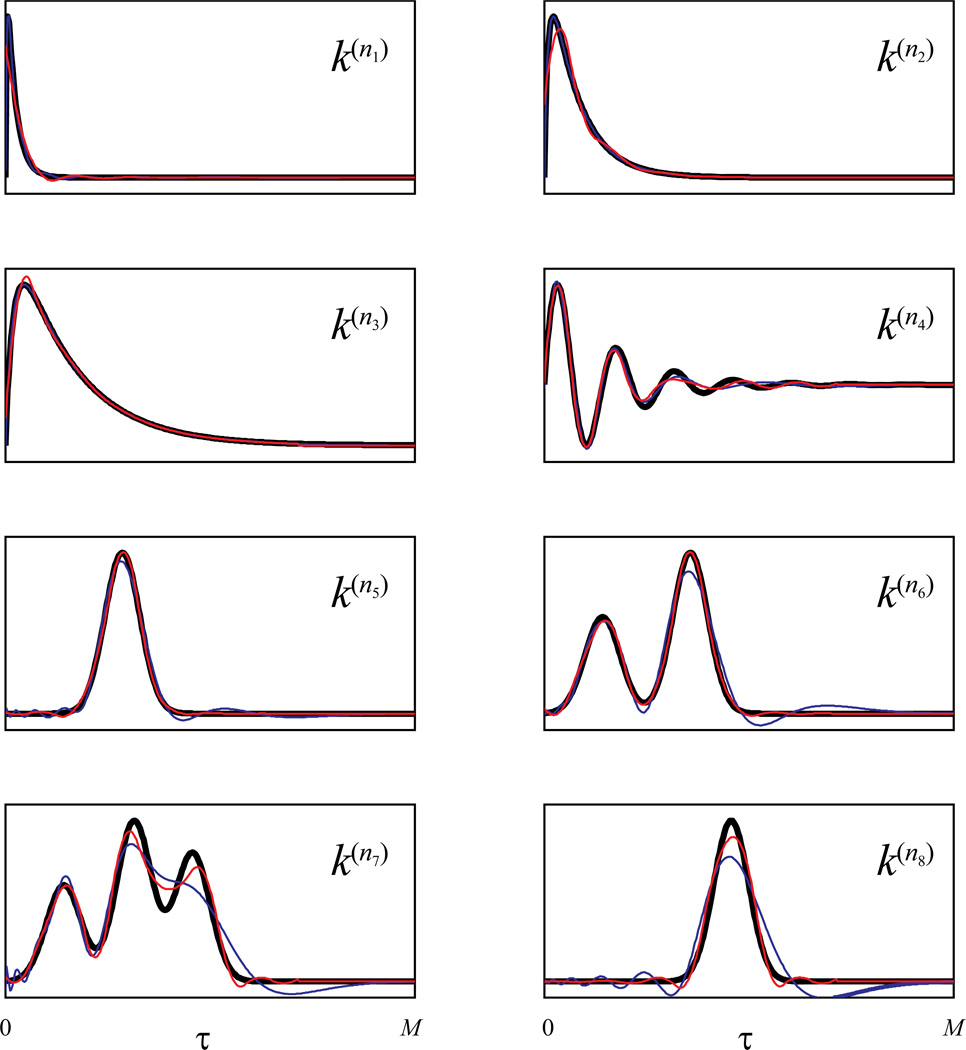
Before testing the entire sparse GFAM algorithm, we first fit directly the designed kernel functions with the basis functions to see the relative strengths and weaknesses of the global basis (i.e., Laguerre basis) and the local basis (i.e., B-spline basis) in fitting different forms of dynamics. Coefficients of the bases are estimated with a least-squares method and then used to reconstruct the kernel functions with the their corresponding basis. Figure 6 illustrates the kernel functions reconstructed with Laguerre basis (J = 13, α = 0.83, blue lines) and B-spline basis (J = 13, red lines), superimposed on the actual kernel functions (black lines). It is evident that both bases can well replicate the kernel functions (Fig. 6). However, the Laguerre basis performs better in the kernel functions with simpler shapes and no delay (e.g., k(n1), k(n2), and k(n3)); the B-spline basis performs better in the kernel functions with more complex shapes (e.g., k(n4), k(n6), and k(n7)) or with delays (e.g., k(n5), and k(n8)). Since the Laguerre basis is global and has an emphasis on the shorter intervals, it tends to generate spurious features in the long intervals when the kernel shape is complex, or in the short intervals when the kernel has a delay. On the other hand, the B-spline basis is local and uniformly distributes on the whole system memory, it generates little spurious features with a slight sacrifice of accuracy in the short intervals.
Figure 6.
Fitting various kernel functions with Laguerre basis functions and B-spline basis functions. Thick black lines: actual kernel functions; thin blue lines: kernel functions fit with Laguerre basis functions; thin red lines: kernel functions fit with B-spline basis functions.
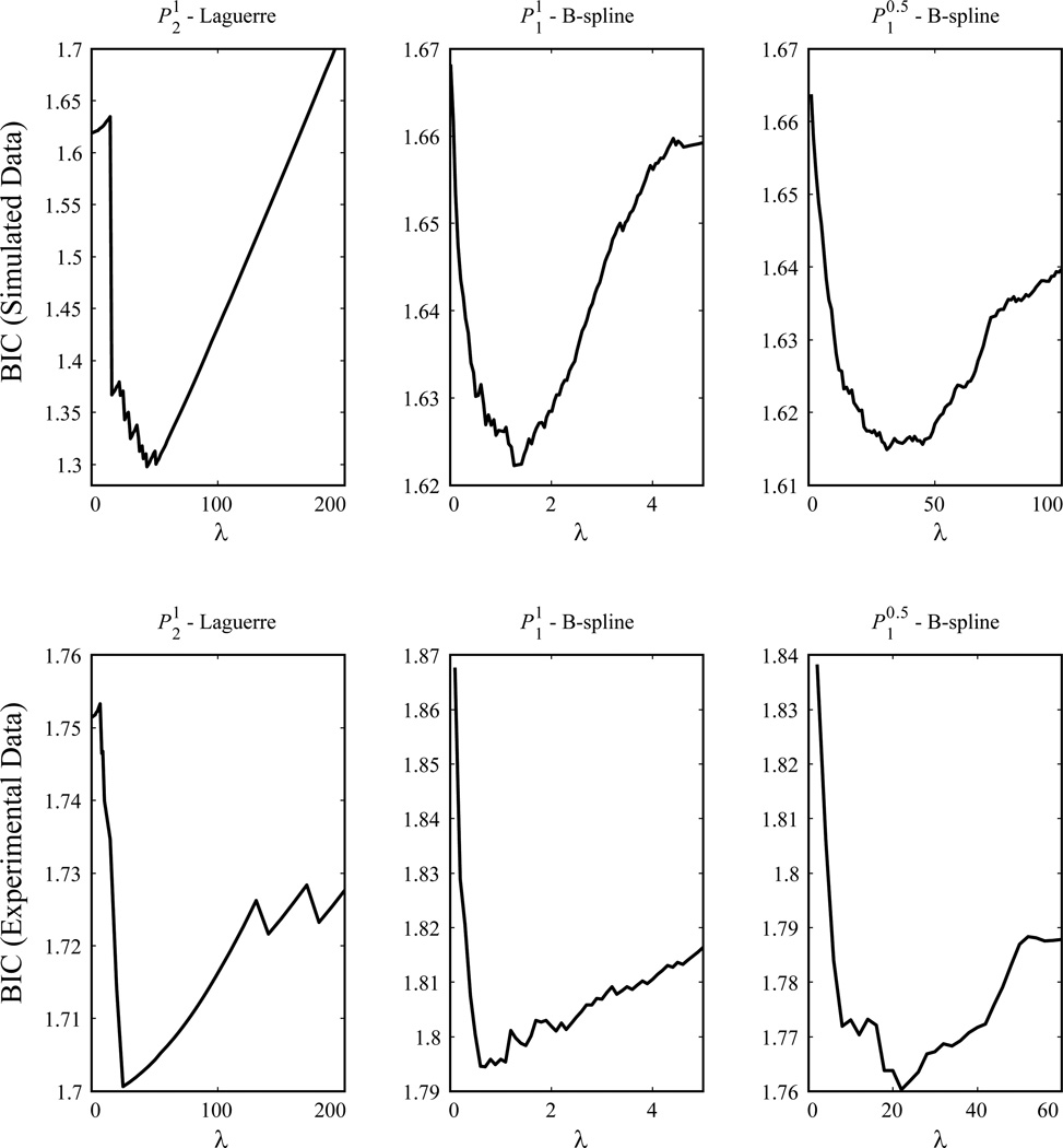
Then we test the whole sparse GFAM algorithm with synthetic input-output data. The system is designed to be 16-input, single-output, with 8 kernel functions to be the functions described above (with the same sequence) and 8 functions to be zeros (i.e., k(3), k(4), k(6), k(8), k(9), k(12), k(13), and k(14)). The zeroth-order kernel is set at −8.5. The input signals are 16 independent Poisson processes with a 10 Hz mean frequency. To produce the single output signal, inputs are convolved with the kernel functions and summed together with the zeroth-order kernel to generate the intermediate variable g(θ(t)). g(θ(t)) is then transformed into the firing probability intensity function θ(t) using the Gaussian error function. The value of output at time t then is realized with a Bernoulli process with a probability equal to θ(t). The data length is 200 s (100000 samples) and the output firing rate is approximately 23.3 Hz. Using these input-output data, kernel functions are estimated with the two sparse GFAM estimation methods. The utilized Laguerre and B-spline bases are the same as above. Tuning parameters λ are chosen with the BIC as described in the Method section (Fig. 7, top panel).
Figure 7.
Choosing tuning parameter λ with Bayesian information criteria (BIC). Top panel: simulated data. Bottom panel: experimental data.
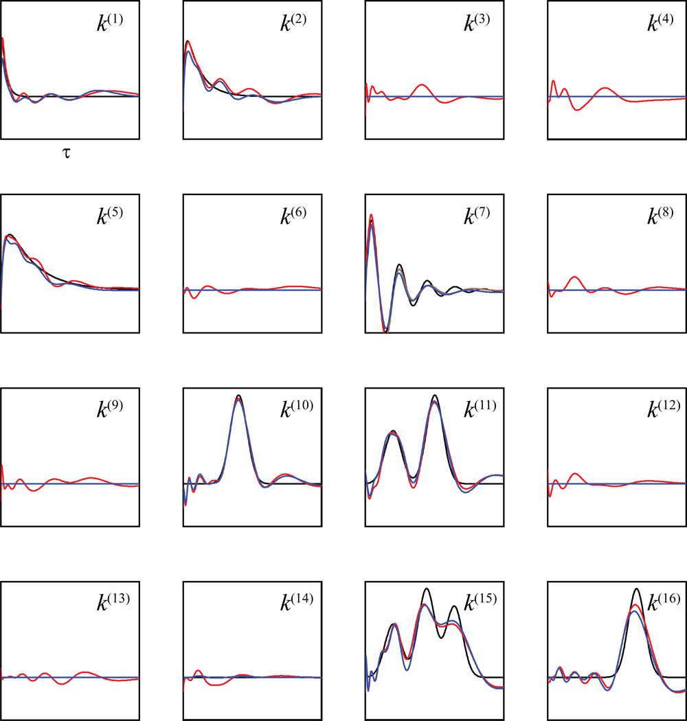
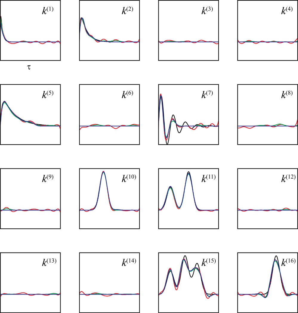
Figure 8 illustrates the kernel functions estimated using and Laguerre basis (blue lines, -Laguerre for short), and maximum likelihood and Laguerre basis (red lines, MLE-Laguerre for short). The true kernel functions are shown in black lines. Since MLE-Laguerre cannot capture global sparsity, it generates spurious values in all zero-valued kernel functions. By contrast, -Laguerre captures the global sparsity with a 100% accuracy. In the non-zero kernel functions, the estimates of -Laguerre and MLE-Laguerre are similar and both fairly accurate. However, the fits are not as good as the direct fits shown in Figure 6, due to the stochastic noise introduced in the synthetic input-output data and the more complicated estimation procedure. This is especially evident in the decaying phases of k(1), k(2) and k(5), and the early delays in k(10) and k(16).
Figure 8.
Estimating the kernel functions and sparsities with Laguerre basis functions. Black: actual kernel functions; Blue lines: functions estimated with ; Red lines: functions estimated with maximum likelihood method.
Figure 9 illustrates the kernel functions estimated using and B-spline basis (blue lines, -B-spline for short), maximum likelihood and B-spline basis (blue lines, MLE-B-spline for short), and and B-spline basis (green lines, -B-spline for short). Results show that neither MLEB-spline nor -B-spline can capture global sparsity since they both yield non-zero values in zero-valued kernels. However, the fits of -B-spline are much better than those of the MLE-B-spline, since the former method is able to achieve a sparse estimate, at least at the local level. By contrast, -B-spline captures the global sparsity with a 100% accuracy. Furthermore, -B-spline also captures the local sparsity in the non-zero kernel functions. The near-zero-valued ranges of these kernels are faithfully replicated by this method.
Figure 9.
Estimating the kernel functions and sparsities with B-spline basis functions. Black: actual kernel functions; Blue lines: functions estimated with ; Red lines: functions estimated with maximum likelihood method. Green lines: functions estimated with .
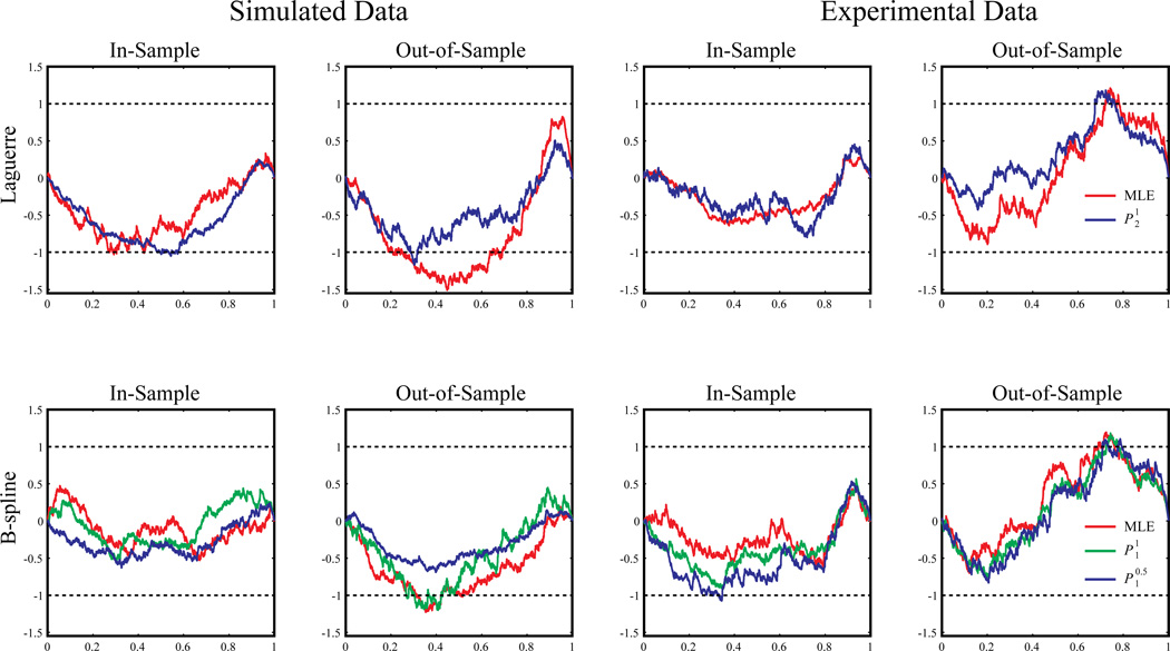
We further evaluate the model goodness-of-fit with the Kolmogorov-Smirnov test based on the time-rescaling theorem. The maximum distances between the KS plots and the diagonal lines are normalized with the distance between the 95% confidence bounds and the diagonal lines to yield the KS scores for each model. In-sample and out-of-sample KS plots and scores are shown in Figure 10 and Table 2. KS scores of the zeroth-order models provide negative controls for the GFAMs. Results show that all models yield a KS score smaller or close to 1. In the in-sample results, model performance decreases as the level of sparsity increases. With the Laguerre basis, the KS score of MLE is smaller than that of the . With the B-spline basis, MLE has the smallest KS score, while has the largest KS score. In the out-of-sample results, model performance increases with the level of sparsity. With the Laguerre basis, the out-performs the MLE. With the B-spline basis, the yields the smallest KS score. These results show that the sparse models alleviate overfitting with a smaller set of model coefficients.
Figure 10.
Model goodness-of-fit shown with horizontal Kolmogorov-Smirnov plots of the estimated models. Dashed black lines represent the 95% confidence bounds.
Table 2.
Model Goodness-of-Fit Evaluated with Kolmogorov-Smirnov Test Based on the Time-Rescaling Theorem
| Simulated Data | Experimental Data | |||||
|---|---|---|---|---|---|---|
| # of Coeff. | KS (In) | KS (Out) | # of Coeff. | KS (In) | KS (Out) | |
| Zeroth-Order | 1 | 28.41 | 29.57 | 1 | 6.06 | 6.12 |
| MLE-Laguerre | 209 | 1.03 | 1.51 | 97 | 0.64 | 1.21 |
| -Laguerre | 105 | 1.05 | 1.17 | 49 | 0.80 | 1.18 |
| MLE-B-spline | 209 | 0.53 | 1.23 | 289 | 0.63 | 1.19 |
| -B-spline | 200 | 0.54 | 1.20 | 61 | 0.92 | 1.18 |
| -B-spline | 45 | 0.63 | 0.69 | 26 | 1.08 | 1.11 |
For each model, KS tests based on the time-rescaling theorem are performed with both simulated and experimental datasets. The maximum distances between the KS plots and the diagonal lines are normalized to yield the KS scores for the comparison between different models using different datasets. KS (In): In-sample KS scores. KS (Out): out-of-sample KS scores. # of Coeff.: total number of coefficients in the model. Zeroth order models only fit the mean firing rate of the output signal.
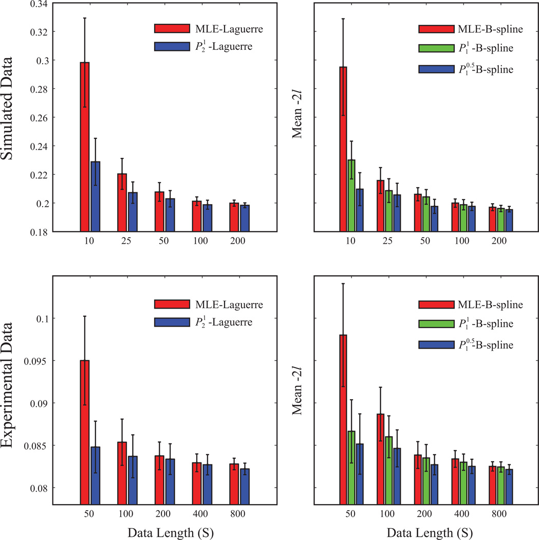
We further compare the performances of the models with different training data length. Models are estimated with 10, 25, 50, 100, and 200 sec of input/output data and then evaluated with the out-of-sample mean negative log-likelihood (Fig. 11). Results show that the penalized methods outperform the MLE method in all data lengths and the improvements become more significant in the shorter data lengths. These results show that the penalized methods allow more reliable estimations from shorter datasets.
Figure 11.
Model performance with different training data lengths. The bars illustrate the means of the out-of-sample negative log-likelihoods; the error bars represent the STDs.
In summary, results of the simulation studies show the advantages of using -Laguerre and -B-spline over other methods with respect to estimation of sparse connectivities.
3.2. Application to Hippocampal CA3-CA1 Modeling
We further apply the GFAM algorithm to experimental data, i.e., simultaneous recordings from the hippocampal CA3-CA1 system. The input and output signals to be modeled are the spike trains recorded from the CA3 and the CA1 regions, respectively.
3.2.1. Experimental Procedures
Multi-unit neural spike trains were recorded from hippocampal CA3 and CA1 regions in male Long-Evans rats performing a memory-dependent, spatial delayed-non-match-to-sample (DNMS) task (Deadwyler et al. 1996; Hampson et al. 1999). Animals performed the task by pressing a single lever presented in one of the two positions in the sample phase (left or right); this event is called the “sample response”. The lever then was retracted and the delay phase initiated; for the duration of the delay phase, the animal was required to nose-poke into a lighted device on the opposite wall. Following termination of the delay the nose-poke light was extinguished, both levers were extended and the animal was required to press the lever opposite to the sample lever; this act is called the “nonmatch response”. If the correct lever was pressed, the animal was rewarded and the trial was completed.
Spike trains were obtained with multi-site recordings from different septo-temporal regions of the hippocampus of rats performing the DNMS task. For each hemisphere of the brain, an array of electrodes was surgically implanted into the hippocampus, with 8 electrodes in the CA3 (input) region and 8 electrodes in the CA1 (output) region. Spikes were sorted and time-stamped with a 25 µs resolution and then downsampled with a 2 ms bin size. For such a bin width, each bin contains a maximum of one spike event, thus retaining the temporal structures of all spike trains. For simplicity, task-dependence, e.g., different events during the DNMS task, is not considered as in a previous study (Song et al., 2011).
3.2.2. Modeling Results
The dataset used in this study is a 800 sec continuous recording of 15 CA3 (input) neurons and one CA1 (output) neurons. It includes 12 left-sample trials, 11 right-sample trials, and the intervals between those trials. During this 800 sec period, the 16 neurons generated 29188, 939, 24098, 834, 546, 20893, 7195, 27006, 355, 674, 156, 607, 414, 655, 2285, and 3093 spikes, respectively. To include the feedback dynamics of the CA1 neuron into the model, the output CA1 spike train is taken as an extra input to the system with a slight modification, i.e., excluding the current spike from the epoch (see Section 2.1 for more details). The model thus predicts the spiking activity of the output CA1 neuron based on the spiking activities of all CA3 neurons and its own spiking history (i.e., the preceding output spikes). The CA3-CA1 kernels are represented as k and the CA1-CA1 feedback kernel is represented as h.
The knot sequence of the B-spline basis is: 0, 0.005, 0.010, 0.015, 0.020, 0.05, 0.1, 0.2, 0.3, 0.4, 0.5, 0.6, 0.7, 0.8, 0.9, 1. Extra knots are added in short intervals to better capture the fast components of the dynamics, i.e., near-instantaneous coupling between the neurons. Since basis functions generally have limited bandwidth, a B-spline basis with uniformly distributed knot sequence will fail to capture this component. The Laguerre parameter of the Laguerre basis is optimized to be 0.94. Six Laguerre basis functions are found to be optimal. Tuning parameter λ are chosen with the BIC as described in the Method section (Fig. 7, bottom panel).
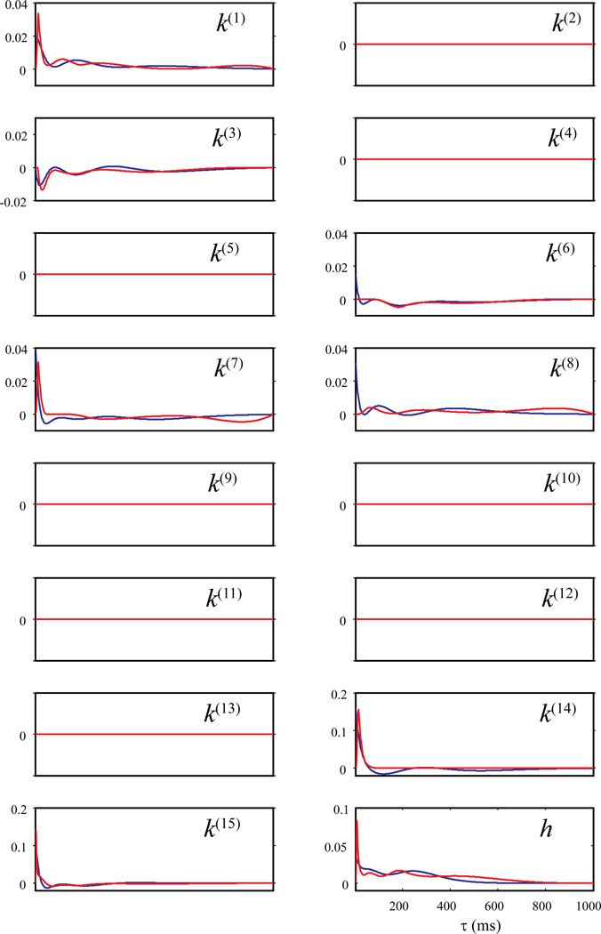
Figure 12 illustrates kernel functions estimated using -Laguerre (blue lines) and -B-spline (red lines). It shows that the two methods yield identical results in global sparsity, i.e., eight (k(2), k(4), k(5), k(9), k(10), k(11), k(12), and k(13)) of the 16 kernels functions are equal to zeros for the whole system memory. For the rest of the kernel functions, the two methods yield similar results with some noticeable differences. In k(1), k(7), k(14), k(15), and h, both methods show a strong positive-going (i.e., facilitatory) component for short intervals (< 40 ms). With -B-spline, these facilitatory components have a peak; while with -Laguerre, these components are monotonic decaying. In k(3), -B-spline and -Laguerre estimates are virtually the same. The kernel functions show a stronger, negative-going (depressive) component for shorter intervals (approximately 0 – 40 ms) followed by a weaker, negative-going component for longer intervals (approximately 40 – 150 ms). In k(6) and k(8), the differences between -B-spline and -Laguerre estimates are relatively larger. -B-spline shows a fast (< 40 ms), monotonic-decaying, positive component in both kernels, while -Laguerre does not. In k(6), both methods show a slower, negative-going component. In k(8), -B-spline shows a peaked positive components at 50 ms, followed by two weaker, slower, positive components. In k(14) and k(15), the -B-spline estimates have considerably shorter system memory (50 ms and 400 ms) compared with the -Laguerre estimates. These reflect the local sparsities captured by the former method.
Figure 12.
Estimating a 15-input, single-output hippocampal CA3-CA1 model using penalized likelihood estimations and basis functions. Blue lines: -Laguerre; Red lines: -B-spline.
The KS scores of the model are shown in Figure 10 and Table 2. In general, the B-spline models yield smaller KS scores than the Laguerre models. Within both of the Laguerre group and the B-spline group, similar to the simulation results, the sparser models perform better in the case of out-of-sample predictions. We further compare the performances of the models with different training data length. Models are estimated with 50, 100, 200, 400, and 800 sec of input/output data (Fig. 11). Similar to the simulation results, it is shown that the penalized methods outperform the MLE method in all data lengths.
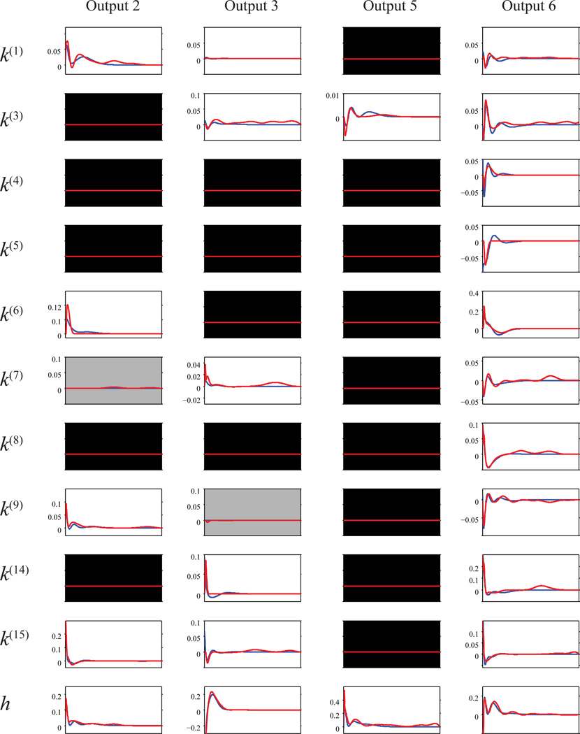
By concatenating multiple sparse MISO models estimate from the same MIMO dataset, sparse MIMO models of the hippocampal CA3-CA1 are obtained. Figure 13 depicts an MIMO model with 17 (CA3) inputs and 6 (CA1) outputs. For simplicity, only the CA3 and CA1 units with significant feedforward kernels are shown. The two methods give very consistent results in the global sparsity. Out of the 102 possible feedforward kernels, 20 feedforward kernels are selected by both methods and 2 extra feedforward kernels are selected by the -B-spline method only. In the selected kernels, the two methods yield similar kernel shapes in general, especially in the larger-magnitude kernels. The -B-spline method picks up more late components in the kernels. All feedback kernels are selected by both methods.
Figure 13.
Sparse MIMO hippocampal CA3-CA1 (17-input, 6-output) model estimated with penalized likelihood estimations and basis functions. Blue lines: -Laguerre; Red lines: -B-spline. Black background: global sparsity estimated with both methods. Gray background: global sparsity estimated with -Laguerre but not -B-spline.
4. Conclusions and Discussion
In this study, we formulate a GFAM framework for the identification of the sparse neural connectivity using spike train data. This GFAM framework has two new features compared to the standard generalized linear model. In terms of model configuration, the GFAM expands the sought kernel functions with a set of basis functions to reduce model complexity. In terms of parameter estimation, the GFAM utilizes various penalized likelihood methods to achieve sparse estimations of the kernel functions. Specifically, group LASSO (i.e., ) and global basis functions (i.e., Laguerre basis) are used to yield sparsity at a group level; group bridge (i.e., ) and local basis functions (i.e., B-spline basis) are adopted to obtain sparsities at both group and within group levels.
There are three major advantages of using sparse models. First, a sparse model facilitates model interpretation by selecting the significant factors in the model. In the case of neural population analysis, it identifies the input neurons that have significant effects on the activity of the output neuron (i.e., global sparsity) and the ranges of system memories of these effects (i.e., local sparsity), and thus reveals and quantifies the functional connectivity within the neural population. Second, a sparse model alleviates overfitting. When a regression model contains a large number of open parameters as in the case of neural population analysis, the parameters tend to fit the noise in addition to the true signal in the training data, and results in an overfitted model. An overfitted model shows poor generalization of the training data and less accurate prediction for an independent testing data. Results show that the sparse models estimated using penalized likelihood methods are more accurate than the full models estimated with the standard maximum likelihood method (Figure 10 and Table 2). Third, model complexity is largely reduced in the sparse model. In the development of cortical neural prostheses, additional power consumption caused by increased model complexity is a major concern (Li et al. 2011; Berger et al. 2012). Applications to the hippocampal CA3-CA1 system in the present study demonstrated that sparse models involve only a subset of the inputs and model coefficients, leading to a much lower computational burden in terms of model prediction. If the model includes higher order nonlinearities (as most models of neural systems must), e.g., nonlinear dynamical interactions between pairs and triplets of spikes from multiple inputs as in the form of a higher order Volterra model, the sparse model can be orders more efficient than the full model (Song et al., 2009).
Two main penalized likelihood methods, i.e., -B-spline and -Laguerre, are introduced in this paper. Standard MLE and -B-spline methods are implemented for comparison. In both simulation and experimental studies, -B-spline shows markedly better performances compared with -Laguerre. This is not surprising since the -B-spline is (1) more flexible in terms of fitting complex and delayed kernel functions (Figure 6), and (2) capable of capturing both global and local sparsities. In addition, the B-spline basis can be further optimized by adjusting the knot sequence to better capture the more important regions of the dynamics. By contrast, -Laguerre captures only global sparsity. Local sparsity can be approximated only with the whole set of basis, which all lack the continuous ranges of zeros. The only tuning parameter of the Laguerre basis, α, controls the overall asymptotic decay rates of the whole basis, but does not change the individual shapes of the basis functions. In general, -B-spline is more flexible and non-parametric than -Laguerre.
However, -Laguerre has one attractive advantage over -B-spline. That is, Laguerre basis, once optimized, often can fit the kernel functions with a relatively smaller number of basis functions. This is due to the fact that most of the commonly observed dynamical neurobiological processes (e.g., post-synaptic current, post-synaptic potential, and short-term synaptic plasticity) have an exponentially decaying shape caused by the damping nature of their temporal dynamics. The Laguerre basis, which has a built-in exponential decay, is more efficient than the B-spline basis in modeling this kind of dynamics. This is shown in the experimental data analysis (Figure 10 and Table 2): MLE-Laguerre achieves a similar level of accuracy with many fewer basis functions compared to the MLE-B-spline, although -Laguerre is not as accurate as the -B-spline. This may not seem to be significant in the case of the first order models described in this paper, but can be a big advantage in higher order models where the number of coefficients increases exponentially with the model order and polynomially with the number of basis functions (Song et al. 2009a).
With the simulated data, -B-spline shows excellent goodness-of-fit with a KS plot having no significant deviations from the true distribution (KS score is 0.63). -Laguerre shows small but significant error (KS score is 1.17). Since the input-output function is designed to be first order and thus -Laguerre has the correct model order, the main source of this error should be from the Laguerre basis. This is verified by the direct fitting of the kernel functions with the Laguerre and B-spline bases, where the Laguerre basis shows some significant bias. With the experimental data, both -Laguerre and -B-spline show small but significant errors (KS scores are 1.21 and 1.11, respectively). Considering the relatively simple shapes of the kernel functions, the most likely cause of such errors could be the nonlinearities (second order and higher) that exist in the data but that are not captured by the first order models. Our previous studies have shown that models of the hippocampal CA3-CA1 often require higher order terms (e.g., at least second order self kernels) to sufficiently capture the input-output dynamics (Song et al., 2006, 2009). Although only described but not implemented in this paper to maintain simplicity, extension of the sparse GFAM to the sparse generalized Volterra model is a natural solution for modeling the higher order nonlinear dynamics and will be the focus of our future studies.
Many other groups in computational neuroscience have used penalized likelihood methods, Bayesian sparsification, and basis functions to estimate the functional connectivities using neural spiking data (Chen et al. 2011; Kelly et al. 2010; Stevenson et al. 2009; Truccolo and Donoghue 2007; Zhao et al. 2012; Pillow et al. 2008; Kass and Ventura 2001; Gerwinn et al. 2010; Park and Pillow 2011). The main innovations of this study are (1) introducing the concepts of global sparsity and local sparsity within the context of neural functional connectivity, (2) providing a unifying framework involving various penalized likelihood estimation methods and basis functions (i.e., global and local bases) to estimate such sparsities. As shown in the results of both simulated and experimental datasets, the standard L1 regularization (LASSO) method can achieve only sparsity at individual variable level and thus does not guarantee global sparsity; the group L1 (group LASSO) approach can achieve global sparsity but not local sparsity. In the Bayesian inference framework developed by Stevenson et al., sparsity is also obtained only at the group level (Stevenson et al. 2009). To the best of our knowledge, the group bridge-local basis approach (e.g., -B-spline) described here is the first successful attempt to the simultaneous identification of both global and local sparsities of neural functional connectivities.
Table 1.
Table of Notations
| Symbols | Meanings |
|---|---|
| x | Input signal |
| y | Output signal |
| H | Causal relation between inputs and the output |
| k0, c0 | Zeroth-order kernel, intercept |
| k(n)(τ) | Kernel function of the nth input at lag τ |
| g | Link function of the model |
| kq | Qth-order kernel function |
| c(n)(j) | Coefficient of the jth basis function of the nth input |
| cq | Qth-order coefficient |
| bj | Basis function |
| B | B-spline basis function |
| η | Knot of the B-spline |
| m | Number of interior knots of a B-spline basis |
| d | Degree of the B-spline |
| L | Laguerre basis function |
| α | Laguerre parameter |
| J | Number of Laguerre basis functions |
| β | The degree of norm in the composite penalty |
| γ | The power of the composite penalty |
| l | Log-likelihood function |
| P | Composite penalty function |
Acknowledgments
D. S., V. Z. M., R. E. H., S. A. D., and T. W. B. were supported in part by the Defense Advanced Research Projects Agency (DARPA) through the Restorative Encoding Memory Integration Neural Device (REMIND) Program, and in part by the National Science Foundation (NSF) through the Biomimetic Microelectronic Systems Engineering Research Center (BMESERC).
D.S., V. Z. M., and T. W. B. were supported in part by the National Institutes of Health (NIH) through the National Institute of Biomedical Imaging and BioEngineering (NIBIB).
C. Y. T, and H. W. were supported in part by the NSF through DMS-0706761 and DMS-0854903.
Appendix
Derivation of matrix R
For logit link function, we have:
Thus, we have:
where
For probit link function, we have:
where
In addition, we have
Thus, we have ∇2l(y|X) = ΦTRΦ, where R = R1 + R2 + R3 + R4.
Contributor Information
Dong Song, Email: dsong@usc.edu.
Haonan Wang, Email: wanghn@stat.colostate.edu.
Catherine Y. Tu, Email: catherine.tu@gmail.com.
Vasilis Z. Marmarelis, Email: marmarelis@hotmail.com.
Robert E. Hampson, Email: rhampson@wfubmc.edu.
Sam A. Deadwyler, Email: sdeadwyl@wfubmc.edu.
Theodore W. Berger, Email: berger@bmsr.usc.edu.
References
- Aertsen AMHJ, Gerstein GL, Habib MK, Palm G. Dynamics of Neuronal Firing Correlation - Modulation of Effective Connectivity. Journal of Neurophysiology. 1989;61(5):900–917. doi: 10.1152/jn.1989.61.5.900. [DOI] [PubMed] [Google Scholar]
- Berger TW, Ahuja A, Courellis SH, Deadwyler SA, Erinjippurath G, Gerhardt GA, et al. Restoring lost cognitive function. IEEE Eng Med Biol Mag. 2005;24(5):30–44. doi: 10.1109/memb.2005.1511498. [DOI] [PubMed] [Google Scholar]
- Berger TW, Hampson RE, Song D, Goonawardena A, Marmarelis VZ, Deadwyler SA. A cortical neural prosthesis for restoring and enhancing memory. Journal of Neural Engineering. 2011;8(4):046017. doi: 10.1088/1741-2560/8/4/046017. [DOI] [PMC free article] [PubMed] [Google Scholar]
- Berger TW, Song D, Chan RHM, Marmarelis VZ. The Neurobiological Basis of Cognition: Identification by Multi-Input, Multioutput Nonlinear Dynamic Modeling. Proceedings of the IEEE. 2010;98(3):356–374. doi: 10.1109/JPROC.2009.2038804. [DOI] [PMC free article] [PubMed] [Google Scholar]
- Berger TW, Song D, Chan RHM, Marmarelis VZ, LaCoss J, Wills J, et al. A Hippocampal Cognitive Prosthesis: Multi-Input, Multi-Output Nonlinear Modeling and VLSI Implementation. IEEE Trans Neural Syst Rehabil Eng. 2012 doi: 10.1109/TNSRE.2012.2189133. in press. [DOI] [PMC free article] [PubMed] [Google Scholar]
- Brown EN, Barbieri R, Ventura V, Kass RE, Frank LM. The time-rescaling theorem and its application to neural spike train data analysis. Neural Computation. 2002;14(2):325–346. doi: 10.1162/08997660252741149. [DOI] [PubMed] [Google Scholar]
- Brown EN, Kass RE, Mitra PP. Multiple neural spike train data analysis: state-of-the-art and future challenges. Nature Neuroscience. 2004;7(5):456–461. doi: 10.1038/nn1228. [DOI] [PubMed] [Google Scholar]
- Chen Z, Putrino DF, Ghosh S, Barbieri R, Brown EN. Statistical Inference for Assessing Functional Connectivity of Neuronal Ensembles With Sparse Spiking Data. [Article] Ieee Transactions on Neural Systems and Rehabilitation Engineering. 2011;19(2):121–135. doi: 10.1109/TNSRE.2010.2086079. [DOI] [PMC free article] [PubMed] [Google Scholar]
- de Boor C. On calculating with B-splines. Journal of Approximation Theory. 1972;6:50–62. [Google Scholar]
- Deadwyler SA, Bunn T, Hampson RE. Hippocampal ensemble activity during spatial delayed-nonmatch-to-sample performance in rats. Journal of Neuroscience. 1996;16(1):354–372. doi: 10.1523/JNEUROSCI.16-01-00354.1996. [DOI] [PMC free article] [PubMed] [Google Scholar]
- Eilers PHC, Marx BD. Flexible smoothing with B-splines and penalties. Statistical Science. 1996;11(2):89–102. [Google Scholar]
- Eldawlatly S, Jin R, Oweiss KG. Identifying Functional Connectivity in Large-Scale Neural Ensemble Recordings: A Multiscale Data Mining Approach. Neural Computation. 2009;21(2):450–477. doi: 10.1162/neco.2008.09-07-606. [DOI] [PMC free article] [PubMed] [Google Scholar]
- Frank IE, Friedman JH. A Statistical View of Some Chemometrics Regression Tools. Technometrics. 1993;35(2):109–135. [Google Scholar]
- Fu WJ. Penalized regression: the bridge versus the lasso. Journal of Computational and Graphical Statistics. 1998;7(3):397–416. [Google Scholar]
- Garofalo M, Nieus T, Massobrio P, Martinoia S. Evaluation of the Performance of Information Theory-Based Methods and Cross-Correlation to Estimate the Functional Connectivity in Cortical Networks. Plos One. 2009;4(8) doi: 10.1371/journal.pone.0006482. [DOI] [PMC free article] [PubMed] [Google Scholar]
- Gerhard F, Pipa G, Lima B, Neuenschwander S, Gerstner W. Extraction of network topology from multi-electrode recordings: is there a small-world effect? Frontiers in Computational Neuroscience. 2011;5:1–13. doi: 10.3389/fncom.2011.00004. [DOI] [PMC free article] [PubMed] [Google Scholar]
- Gerwinn S, Macke JH, Bethge M. Bayesian inference for generalized linear models for spiking neurons. Frontiers in Computational Neuroscience. 2010;4 doi: 10.3389/fncom.2010.00012. [DOI] [PMC free article] [PubMed] [Google Scholar]
- Gourevitch B, Eggermont JJ. Evaluating information transfer between auditory cortical neurons. Journal of Neurophysiology. 2007;97(3):2533–2543. doi: 10.1152/jn.01106.2006. [DOI] [PubMed] [Google Scholar]
- Hampson RE, Simeral JD, Deadwyler SA. Distribution of spatial and nonspatial information in dorsal hippocampus. Nature. 1999;402(6762):610–614. doi: 10.1038/45154. [DOI] [PubMed] [Google Scholar]
- Harris KD, Csicsvari J, Hirase H, Dragoi G, Buzsaki G. Organization of cell assemblies in the hippocampus. Nature. 2003;424(6948):552–556. doi: 10.1038/nature01834. [DOI] [PubMed] [Google Scholar]
- Haslinger R, Pipa G, Brown E. Discrete Time Rescaling Theorem: Determining Goodness of Fit for Discrete Time Statistical Models of Neural Spiking. Neural Computation. 2010;22(10):2477–2506. doi: 10.1162/NECO_a_00015. [DOI] [PMC free article] [PubMed] [Google Scholar]
- Hille B. Ionic Channels of Excitable Membranes. Sunderland, Mass: Sinauer Associates; 1992. [Google Scholar]
- Hines ML, Carnevale NT. Expanding NEURON's repertoire of mechanisms with NMODL. Neural Computation. 2000;12(5):995–1007. doi: 10.1162/089976600300015475. [DOI] [PubMed] [Google Scholar]
- Huang J, Ma S, Xie H, Zhang C-H. A group bridge approach for variable selection. Biometrika. 2009;96(4):1024–1024. doi: 10.1093/biomet/asp020. [DOI] [PMC free article] [PubMed] [Google Scholar]
- Ito S, Hansen ME, Heiland R, Lumsdaine A, Litke AM, Beggs JM. Extending Transfer Entropy Improves Identification of Effective Connectivity in a Spiking Cortical Network Model. Plos One. 2011;6(11) doi: 10.1371/journal.pone.0027431. [DOI] [PMC free article] [PubMed] [Google Scholar]
- Johnston D. Foundations of Cellular Neurophysiology. Cambridge: The MIT Press; 1999. [Google Scholar]
- Kass RE, Ventura V. A spike-train probability model. Neural Computation. 2001;13(8):1713–1720. doi: 10.1162/08997660152469314. [DOI] [PubMed] [Google Scholar]
- Kelly RC, Smith MA, Kass RE, Lee TS. Accounting for network effects in neuronal responses using L1 regularized point process models. NIPS - Advances in Neural Information Processing Systems. 2010;23:1099–1107. [PMC free article] [PubMed] [Google Scholar]
- Kim S, Putrino D, Ghosh S, Brown EN. A Granger Causality Measure for Point Process Models of Ensemble Neural Spiking Activity. Plos Computational Biology. 2011;7(3) doi: 10.1371/journal.pcbi.1001110. [DOI] [PMC free article] [PubMed] [Google Scholar]
- Kutner MH, Nachtsheim CJ, Neter J, Li W. Applied Linear Statistical Models. 5th ed. Boston: McGraw-Hill/Irwin; 2004. [Google Scholar]
- Li WXY, Chan RHM, Zhang W, Cheung RCC, Song D, Berger TW. High-Performance and Scalable System Architecture for the Real-Time Estimation of Generalized Laguerre-Volterra MIMO Model From Neural Population Spiking Activity. Emerging and Selected Topics in Circuits and Systems, IEEE Journal on. 2011;1(4):489–501. [Google Scholar]
- Li L, Park IM, Seth S, Sanchez JC, Principe JC. Functional Connectivity Dynamics Among Cortical Neurons: A Dependence Analysis. Neural Systems and Rehabilitation Engineering, IEEE Transactions on. 2012;20(1):18–30. doi: 10.1109/TNSRE.2011.2176749. [DOI] [PubMed] [Google Scholar]
- Marmarelis VZ. Identification of nonlinear biological systems using Laguerre expansions of kernels. Ann Biomed Eng. 1993;21(6):573–589. doi: 10.1007/BF02368639. [DOI] [PubMed] [Google Scholar]
- Marmarelis VZ. Nonlinear Dynamic Modeling of Physiological Systems (IEEE Press Series on Biomedical Engineering) Hoboken: Wiley-IEEE Press; 2004. [Google Scholar]
- McCullagh P, Nelder JA. Generalized Linear Models. 2nd ed. Boca Raton, FL: Chapman & Hall/CRC; 1989. [Google Scholar]
- Nedungadi AG, Rangarajan G, Jain N, Ding MZ. Analyzing multiple spike trains with nonparametric granger causality. Journal of Computational Neuroscience. 2009;27(1):55–64. doi: 10.1007/s10827-008-0126-2. [DOI] [PubMed] [Google Scholar]
- Ogura H. Orthogonal functionals of the Poisson process. Information Theory, IEEE Transactions on. 1972;18(4):473–481. [Google Scholar]
- Okatan M, Wilson MA, Brown EN. Analyzing functional connectivity using a network likelihood model of ensemble neural spiking activity. Neural Computation. 2005;17(9):1927–1961. doi: 10.1162/0899766054322973. [DOI] [PubMed] [Google Scholar]
- Paninski L. Estimation of Entropy and Mutual Information. Neural Computation. 2003;15(6):1191–1253. [Google Scholar]
- Paninski L, Pillow JW, Simoncelli EP. Maximum likelihood estimation of a stochastic integrate-and-fire neural encoding model. Neural Computation. 2004;16(12):2533–2561. doi: 10.1162/0899766042321797. [DOI] [PubMed] [Google Scholar]
- Park M, Pillow JW. Receptive Field Inference with Localized Priors. Plos Computational Biology. 2011;7(10) doi: 10.1371/journal.pcbi.1002219. [DOI] [PMC free article] [PubMed] [Google Scholar]
- Pillow JW, Paninski L, Uzzell VJ, Simoncelli EP, Chichilnisky EJ. Prediction and decoding of retinal ganglion cell responses with a probabilistic spiking model. Journal of Neuroscience. 2005;Vol. 25:11003–11013. doi: 10.1523/JNEUROSCI.3305-05.2005. [DOI] [PMC free article] [PubMed] [Google Scholar]
- Pillow JW, Shlens J, Paninski L, Sher A, Litke AM, Chichilnisky EJ, et al. Spatio-temporal correlations and visual signalling in a complete neuronal population. Nature. 2008;454(7207):U995–U937. doi: 10.1038/nature07140. [DOI] [PMC free article] [PubMed] [Google Scholar]
- Quinn CJ, Coleman TP, Kiyavash N, Hatsopoulos NG. Estimating the directed information to infer causal relationships in ensemble neural spike train recordings. Journal of Computational Neuroscience. 2011;30(1):17–44. doi: 10.1007/s10827-010-0247-2. [DOI] [PMC free article] [PubMed] [Google Scholar]
- Reed JL, Kaas JH. Statistical analysis of large-scale neuronal recording data. Neural Networks. 2010;23(6):673–684. doi: 10.1016/j.neunet.2010.04.005. [DOI] [PMC free article] [PubMed] [Google Scholar]
- Schmidt M, Fung G, Rosales R. Fast optimization methods for L1 regularization: A comparative study and two new approaches. In: Kok JN, Koronacki J, DeMantaras RL, Matwin S, Mladenic D, Skowron A, editors. Machine Learning: ECML 2007, Proceedings. Vol. 4701. Berlin: Springer-Verlag Berlin; 2007. pp. 286–297. (Lecture Notes in Artificial Intelligence). [Google Scholar]
- Schmidt M, Murphy K, Fung G, Rosales R Ieee. Structure learning in random fields for heart motion abnormality detection. 2008 Ieee Conference on Computer Vision and Pattern Recognition, Vols 1–12; (Proceedings - Ieee Computer Society Conference on Computer Vision and Pattern Recognition); 2008. pp. 203–210. [Google Scholar]
- Schumaker L. Spline Functions: Basic Theory(American Scientist) Wiley; 1980. [Google Scholar]
- Schwarz G. Estimating the Dimension of a Model. Annals of Statistics. 1978;6:461–464. [Google Scholar]
- So K, Koralek AC, Ganguly K, Gastpar MC, Carmena JM. Assessing functional connectivity of neural ensembles using directed information. Journal of Neural Engineering. 2012;9(2):026004. doi: 10.1088/1741-2560/9/2/026004. [DOI] [PubMed] [Google Scholar]
- Song D, Berger TW. Identification of Nonlinear Dynamics in Neural Population Activity. In: Oweiss KG, editor. Statistical Signal Processing for Neuroscience and Neurotechnology. Boston: McGraw-Hill/Irwin; 2009. [Google Scholar]
- Song D, Chan RH, Marmarelis VZ, Hampson RE, Deadwyler SA, Berger TW. Nonlinear dynamic modeling of spike train transformations for hippocampal-cortical prostheses. IEEE Trans Biomed Eng. 2007;54(6 Pt 1):1053–1066. doi: 10.1109/TBME.2007.891948. [DOI] [PubMed] [Google Scholar]
- Song D, Chan RH, Marmarelis VZ, Hampson RE, Deadwyler SA, Berger TW. Nonlinear modeling of neural population dynamics for hippocampal prostheses. Neural Networks. 2009a;22(9):1340–1351. doi: 10.1016/j.neunet.2009.05.004. [DOI] [PMC free article] [PubMed] [Google Scholar]
- Song D, Marmarelis VZ, Berger TW. Parametric and non-parametric modeling of short-term synaptic plasticity. Part I: Computational study. Journal of Computational Neuroscience. 2009b;26(1):1–19. doi: 10.1007/s10827-008-0097-3. [DOI] [PMC free article] [PubMed] [Google Scholar]
- Song D, Wang Z, Marmarelis VZ, Berger TW. Parametric and non-parametric modeling of short-term synaptic plasticity. Part II: Experimental study. Journal of Computational Neuroscience. 2009c;26(1):21–37. doi: 10.1007/s10827-008-0098-2. [DOI] [PMC free article] [PubMed] [Google Scholar]
- Song D, Chan RHM, Marmarelis VZ, Hampson RE, Deadwyler SA, Berger TW. Estimation and statistical validation of event-invariant nonlinear dynamic models of hippocampal CA3-CA1 population activities; Proceedings of the IEEE EMBS Conference; 2011. pp. 3330–3333. [DOI] [PubMed] [Google Scholar]
- Stevenson IH, Rebesco JM, Hatsopoulos NG, Haga Z, Member LEM, Kording KP. Bayesian inference of functional connectivity and network structure from spikes. IEEE Transactions on Neural Systems and Rehabilitation Engineering. 2009;17(3):203–213. doi: 10.1109/TNSRE.2008.2010471. [DOI] [PMC free article] [PubMed] [Google Scholar]
- Stevenson IH, Rebesco JM, Miller LE, Kording KP. Inferring functional connections between neurons. Current Opinion in Neurobiology. 2008;18(6):582–588. doi: 10.1016/j.conb.2008.11.005. [DOI] [PMC free article] [PubMed] [Google Scholar]
- Tibshirani R. Regression shrinkage and selection via the Lasso. Journal of the Royal Statistical Society Series B-Methodological. 1996;58(1):267–288. [Google Scholar]
- Truccolo W, Donoghue JP. Nonparametric modeling of neural point processes via stochastic gradient boosting regression. Neural Computation. 2007;19(3):672–705. doi: 10.1162/neco.2007.19.3.672. [DOI] [PubMed] [Google Scholar]
- Truccolo W, Eden UT, Fellows MR, Donoghue JP, Brown EN. A point process framework for relating neural spiking activity to spiking history, neural ensemble, and extrinsic covariate effects. Journal of Neurophysiology. 2005;93(2):1074–1089. doi: 10.1152/jn.00697.2004. [DOI] [PubMed] [Google Scholar]
- Tu CY, Song D, Breidt FJ, Berger TW, Wang H. Functional model selection for sparse binary time series with multiple inputs. In: Holan SH, Bell WR, McElroy TS, editors. Economic Time Series: Modeling and Seasonality. Boca Raton, Florida: Chapman and Hall/CRC; 2012. [Google Scholar]
- Vidne M, Ahmadian Y, Shlens J, Pillow JW, Kulkarni J, Litke AM, et al. Modeling the impact of common noise inputs on the network activity of retinal ganglion cells. Journal of Computational Neuroscience. 2012;33(1):97–121. doi: 10.1007/s10827-011-0376-2. [DOI] [PMC free article] [PubMed] [Google Scholar]
- Yuan M, Lin Y. Model selection and estimation in regression with grouped variables. Journal of the Royal Statistical Society Series B-Statistical Methodology. 2006;68:49–67. [Google Scholar]
- Zanos TP, Courellis SH, Berger TW, Hampson RE, Deadwyler SA, Marmarelis VZ. Nonlinear modeling of causal interrelationships in neuronal ensembles. IEEE Trans Neural Syst Rehabil Eng. 2008;16(4):336–352. doi: 10.1109/TNSRE.2008.926716. [DOI] [PMC free article] [PubMed] [Google Scholar]
- Zhao MY, Batista A, Cunningham JP, Chestek C, Rivera-Alvidrez Z, Kalmar R, et al. An L (1)-regularized logistic model for detecting short-term neuronal interactions. Journal of Computational Neuroscience. 2012;32(3):479–497. doi: 10.1007/s10827-011-0365-5. [DOI] [PubMed] [Google Scholar]
- Zucker RS, Regehr WG. Short-term synaptic plasticity. Annual Review of Physiology. 2002;64:355–405. doi: 10.1146/annurev.physiol.64.092501.114547. [DOI] [PubMed] [Google Scholar]


