Beyond Gaussians: a study of single spot modeling for scanning proton dose calculation

Abstract

Active spot scanning proton therapy is becoming increasingly adopted by proton therapy centers worldwide. Unlike passive-scattering proton therapy, active spot scanning proton therapy, especially intensity-modulated proton therapy, requires proper modeling of each scanning spot to ensure accurate computation of the total dose distribution contributed from a large number of spots. During commissioning of the spot scanning gantry at the Proton Therapy Center in Houston, it was observed that the long-range scattering protons in a medium may have been inadequately modeled for high-energy beams by a commercial treatment planning system, which could lead to incorrect prediction of field-size effects on dose output. In the present study, we developed a pencil-beam algorithm for scanning-proton dose calculation by focusing on properly modeling individual scanning spots. All modeling parameters required by the pencil-beam algorithm can be generated based solely on a few sets of measured data. We demonstrated that low-dose halos in single-spot profiles in the medium could be adequately modeled with the addition of a modified Cauchy-Lorentz distribution function to a double-Gaussian function. The field-size effects were accurately computed at all depths and field sizes for all energies, and good dose accuracy was also achieved for patient dose verification. The implementation of the proposed pencil beam algorithm also enabled us to study the importance of different modeling components and parameters at various beam energies. The results of this study may be helpful in improving dose calculation accuracy and simplifying beam commissioning and treatment planning processes for spot scanning proton therapy.

1. Introduction

The number of proton centers worldwide with spot scanning beams is expected to increase dramatically in near future. Intensity modulated proton therapy (IMPT) has been shown to potentially reduce the dose to normal tissues while maintaining or increasing the prescribed dose delivered to a tumor compared with the passive scattering proton therapy (PSPT) or intensity modulated radiation therapy using x-rays (Lomax et al. 1999, Weber et al. 2004, Muzik et al. 2008, Merchant et al. 2008, Zhang et al. 2010, Ares et al. 2010). As a result, IMPT may further increase the chance of tumor control and improve the quality of life for cancer patients. In active spot scanning proton therapy, hundreds and thousands of narrow, nearly mono-energetic proton beams called scanning spots are delivered from different angles or fields to cover specified tumor volumes laterally via magnetic scanning and longitudinally via varying proton energies. In IMPT, because scanning spots are individually weighted, spots from all fields must be properly superimposed or combined to provide uniform or other desired dose distribution inside targets. In this technique, the dose distribution from each field may not necessarily be uniform, and the weights and spot arrangements can fluctuate drastically. Unlike in broad-beam scenarios of PSPT, properly modeling single scanning spots is crucial in spot scanning beams to ensure that the final dose distribution accumulated from a large number of spot contributions is accurate.

For relatively high proton energies, a non-negligible proportion of protons undergo long-range scatterings caused mainly by nuclear interactions with the medium. As a result, a low-dose halo exists over an extended distance from the central axis of a scanning spot. If low dose halos are not properly modeled, the resulting errors may accumulate over a large number of spots located at a large distance from the point of interest. These errors may account for up to 15% of the total dose (Pedroni et al. 2005). It was observed that the doses measured at the centers of square fields had different values at different field sizes despite the fact that all of the spots were evenly distributed and equally weighted for all field sizes, the so-called “field-size effect” (Inaniwa et al. 2009, Sawakuchi et al. 2010). In scanning proton therapy, small fields containing as few as one or two spots in an energy layer are often encountered, for example, near the distal end of a target. Dose calculation calibrated under broad beam settings with large numbers of spots may become inaccurate for these small fields. If low-dose halos are not adequately modeled, calculations in narrow fields may be problematic by using some fixed calibration factors possibly derived for broad fields. In turn, this may affect dose calculation accuracy especially for IMPT in which spot arrangements may be highly irregular and the field sizes of the energy layers may vary dramatically.

Pencil beam dose calculation algorithms have been described in several publications for proton beams (Petti 1992, Hong et al. 1996, Deasy 1998, Schaffner et al. 1999, Russell et al. 2000, Soukup et al. 2005, Ulmer and Schaffner 2011, Grevillot et al. 2011). For handling of large-angle scatters (e.g., secondary protons and heavy particles resulting from nuclear interactions), our clinical treatment planning system (TPS) (Eclipse 8.9, Varian Medical Systems, Alta Palo, CA) uses another Gaussian in addition to a double-Gaussian function describing the primary and recoil protons to model the pencil beam distribution in a medium (Ulmer and Schaffner 2011). In addition, the lateral fluence distributions (i.e., in-air spot lateral profiles) are also described using a double-Gaussian function. During the scanning beam clinical commissioning, we observed that the doses measured at the centers of square fields as a function of field size could not be simultaneously, accurately predicted at multiple depths by our clinical TPS. The largest discrepancy was found at medium depths for high energy pencil beams (Zhu et al. 2011), despite the fact that many Gaussians (two for in-air and three for in-medium) were used by the dose algorithm. As a workaround, the PTC-H physics team had to create separate sets of modeling parameters for large and small field sizes to ensure IMPT dose calculation accuracy in the TPS. The relative weights of Gaussian components were manually adjusted by trial and error to fit the field-size effects measured in water. As a result, however, the in-air profiles of individual scanning spots computed using the modified parameters may have deviated from the actual profiles.

In this study, we developed a pencil beam algorithm for spot scanning proton dose calculation by focusing on adequate modeling of individual scanning spots in a medium. All of the modeling parameters can be generated based solely on a few sets of measured data. We demonstrated that low-dose halos of single-spot profiles in the medium could be accurately modeled with the addition of a modified Cauchy-Lorentz function to the two Gaussian functions. Because in-air and in-water profiles of single scanning spots were adequately described, with just one set of modeling parameters the field size effects were accurately calculated at all depths and field sizes for all energies, and good accuracy was also achieved for actual patient dose verification. This implementation of the proposed pencil beam algorithm also enabled us to study the importance of different modeling components and parameters at various beam energies. This work may be useful in improving dose accuracy and simplifying beam commissioning and treatment planning processes for spot scanning proton therapy.

2. Methods and materials

2.1. Measurement data

The integral depth dose (IDD) distribution in water can be measured or generated by using a Monte Carlo simulation. Optionally, the IDDs can be fit into analytical formulas for convenient handling (Bortfeld 1997). The IDD data used in our clinical proton TPS was generated by using Monte Carlo simulations and verified by the measurements of selected energies. As part of our scanning proton dose calculation algorithm research, an improved analytic formula was developed based on Bortfeld’s work (Bortfeld 1997), and designed to generate a full set of IDD data for all proton energies required for our TPS commissioning from the measured IDD data at only a few selected energies (Zhang et al. 2011). We adopted the same computed tomography (CT) calibration table that contains stopping power ratios relative to water for the clinical range of Hounsfield units. These ratios scale the geometric depth to compute the water equivalent depth (WED), so the depth dose distribution in water can be associated to that in a patient or a heterogeneous medium.

In-air spot sizes in terms of full width at half maximum (FWHM) were measured using both radiochromic film and a 2-mm-diameter pin-point ionization chamber at the iso-center and ±10 and ±20 cm from the iso-center along the beam direction for selected energies during commissioning our scanning proton beam gantry (Gillin et al. 2010). The spot size at any position z along the beam axis can be determined by fitting the function $f(z)=\sqrt{\frac{A}{2}+B·z+\frac{c}{2}·z^2}$ to the measured values, where A, B, C are free fitting parameters (Schaffner 2008). Under the beam’s eye view system, spot size in the x and y directions in the transverse plane may be different. (In a beam’s eye view system, the z-axis is parallel to the central axis of the beam; it starts from the iso-center and points to the source) For simplicity, we assume spot sizes are isotropic and the averages of spot sizes in the x and y directions are used for our implementation. For example, the in-air spot size in FWHM at the isocenter used in the field size study as well as in the TPS configuration is 12.8 mm for 221.8 MeV, 15 mm for 181.1 MeV and 34.3 mm for 72.5 MeV. The standard deviation σ_in-airof an in-air single-spot profile modeled by a single Gaussian function can be derived by using the relation σ = FWHM/2.355.

Correctly acquiring the low-dose halos in single-spot profiles is crucial to correcting IDD data for nuclear interactions (Zhang et al. 2011) and generating modeling parameters for in-medium single-spot profiles. Anand et al (2011) measured single-spot lateral profiles in water over extended lateral distances from the spot central axis at multiple depths covering low-dose halo regions for many of the 94 scanning proton energies available at the PTC-H (72.5–221.8 MeV). To accommodate profile measurements over large lateral distances at various depths, a PTW MP3 water tank with three-dimensional scanning and control systems (MEPHYSTO mc² software program; PTW, Freiberg, Germany) was used. The reference pin-point ionization chamber was carefully positioned relative to the measuring chamber and moved occasionally during profiling to minimize perturbation of the beam and, at the same time, ensure that the signal of the low-dose halos are properly detected (Anand et al. 2011, Sawakuchi et al. 2010).

Because the interpolation procedures for parameter generation worked well in our dose calculation implementation, overall measurement data, such as IDDs and in-water spot profiles only for a relatively small subset of all 94 energies (fewer than 15 energies), would be needed to determine all parameters required by the proposed algorithm.

2.2. In-air single-spot profiles

The information of the source and beam-line devices upstream from the patient is characterized using in-air lateral spot profiles that are modeled with the two-dimensional (2D) Gaussian funtion: ${\text{LAT}}_{\text{in-air}}(x_0,y_0)=\frac{1}{2\pi {\sigma }_x{\sigma }_y}{e}^{-{(x-x_0)}^2/2{\sigma }_{\text{x,in-air}}^2}{e}^{-{(y-y_0)}^2/2{\sigma }_{\text{y,in-air}}^2}$, where the standard deviations σ_x and σ_y are dependent on the distance from the source to the measurement plane and were set to be equal in our implementation for the purposes of simplicity. We found that the approximation of an in-air profile using one Gaussian function was sufficient in terms of the final calculated dose accuracy when a modified Cauchy-Lorentz function is used in addition to two Gaussian functions to describe dose distribution in medium.

2.3. In-water single-spot profiles

Once a spot enters a patient or phantom, the single Gaussian function characterizing the spot in air continues to be widened by the multiple Coulomb scattering and nuclear interactions in the medium. Increases in its standard deviation contributed by in-patient scattering as a function of the WED can be evaluated by using Hong’s published lookup tables calculated using the generalized Highland approximation (Hong et al. 1996, Gottschalk 2004). Here the in-air Gaussian component broadened by in-patient scattering is called the first or the primary Gaussian component ${\sigma }_{1G}^2={\sigma }_{\text{in−air}}^2(z)+{\sigma }_{\text{patient}}^2(\text{WED})$. In addition to the primary Gaussian component, a second Gaussian function with a large standard deviation and a modified Cauchy-Lorentz distribution function were used to describe the long-range scatters caused by nuclear interaction and large-angle Coulomb scattering that are not accounted using the primary Gaussian component. Figure 1 shows the lateral spot profiles in water modeled using the first and second Gaussian and modified Cauchy-Lorentz components. Because the source-to-axis distance adopted at the PTC-H is relatively large comparing to the patient dimension and the beam width varies generally less than 10% from the surface of the patient to the end of the beam range (Sawakuchi et al. 2010), the weights and widths of the second Gaussian component and modified Cauchy-Lorentz component can be approximated as functions of the WED in the patient. For a spot centered at (x₀, y₀) in the beam’s eye view system, the lateral spot profile (LAT_j) for the j^th scanning spot comprises three terms corresponding to the three modeling components:

$${\text{LAT}}_{\text{j}}(\text{x}.\text{y})=\frac{1-W_{2G}-W_{\text{cauchy}}}{2\pi {\sigma }_{1G}^2}{e}^{-{(x-x_0)}^2/2{\sigma }_{1G}^2}{e}^{-{(y-y_0)}^2/2{\sigma }_{1G}^2}+\frac{W_{2G}}{2\pi {\sigma }_{2G}^2}{e}^{-{(x-x_0)}^2/2{\sigma }_{2G}^2}{e}^{-{(y-y_0)}^2/2{\sigma }_{2G}^2}+\frac{W_{\text{cauchy}}·T(x,y)}{\int {\int }_{-\infty }^{+\infty }T(x,y)\text{dxdy}}$$

W_2G and W_cauchy are weights of the second Gaussian and modified Cauchy component respectively. σ_1G and σ_2G denote the standard deviations of the first and second Gaussian component respectively. In their widely adopted pencil beam algorithm for IMPT, Soukup et al (2005) described formulae that calculates the contribution of nuclear correction W_nuc and σ_nuc based on the Monte Carlo simulations:

$$\begin{array}{l}{W}_{\text{nuc}}=\left[0.052·\log \left(1.13+\frac{\text{WED}}{11.2-0.023·R}\right)+0.35·\frac{0.0017·R^2-R}{{(R+3)}^2-WE{D}^2}-1.61\times {10}^{-9}·\text{WED}·{(R+3)}^2\right]\\ {\sigma }_{\text{nuc}}=\left[2.85+0.0014·R·\log (\text{WED}+3)+0.06·\text{WED}-7.4\times {10}^{-5}·{\text{WED}}^2-0.22·\frac{R}{{(\text{WED}-R-5)}^2}\right].\end{array}$$

Figure 1.

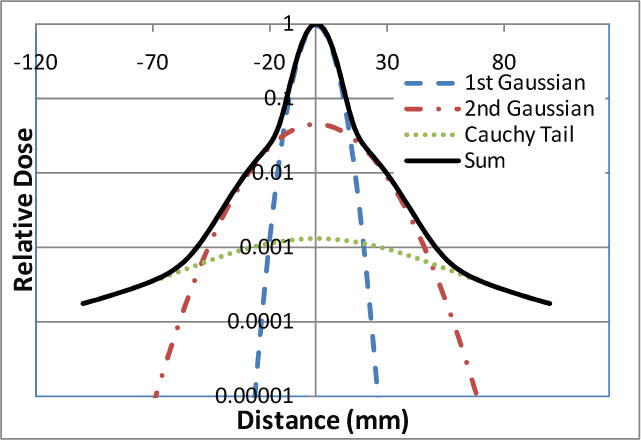
Lateral profile of a scanning spot in water modeled using the first and second Gaussian components and modified Cauchy-Lorentz function.

Here the proton range in water for the given nominal energy is denoted by R, and the depth in water is denoted by WED for notation consistency. (Note: the coefficient 7.4⁻⁵ is changed to 7.4 × 10⁻⁵ in the original formula of σ_nuc based on a formula verification.) Soukup’s original formulae was modified by appending a scaling function to better model our proton scanning beam characteristics, and the contribution of long-range in-patient scattering with the relative weight W_2G and width σ_LR can be expressed using the formulae

$$\begin{array}{c}{W}_{2G}=W_{\text{nuc}}·\text{a}{\left(\frac{\text{WED}}{R}\right)}^p\\ {\sigma }_{\text{LR}}={\sigma }_{\text{nuc}}·\text{a}\prime {\left(\frac{\text{WED}}{R}\right)}^{p\prime }\end{array}$$

where a, p, a′ and p′ are fitting parameters that can be derived from the in-water spot profile measurements. The width of the second Gaussian component can then be computed as ${\sigma }_{2G}^2={\sigma }_{1G}^2(z,\text{WED})+{\sigma }_{\text{LR}}^2(\text{WED})$. The remainder of the low-dose halo is modeled using the modified Cauchy-Lorentz function:

$$T(x,y)=(1-A{e}^{-[{(x-x_0)}^2+{(y-y_0)}^2]/2b^2{\sigma }_{2G}^2})/[\pi b(\frac{{(x-x_0)}^2+{(y-y_0)}^2}{b^2}+1)],$$

where $A=\frac{2{\sigma }_{2G}^2}{2{\sigma }_{2G}^2+1\prime }$ and b is the half width at half maximum (HWHM) of the Cauchy-Lorentz distribution.

2.4. Total dose distribution

A relatively large source-to-axis distance of about 3 m was adopted for the scanning beam nozzle at the PTC-H. Hence, the angular divergence of scanning spots is small, and spots can be considered parallel incident. The IDD of a scanning spot is scaled by the water-equivalent thickness computed from the source to the dose voxel of interest, and the dose can then be computed for the voxel by adding the dose contributions from all spots with consideration of their lateral distributions shown using the ray casting model described by Schaffner et al (1999),

$$D(x,y,z)={\displaystyle \sum }_{j=1}^{N_b}\left[w_j{\text{IDD}}_j(\text{WED}(x,y,z)){{\displaystyle \int }}_{x-\text{Δ}x/2}^{x+\text{Δ}x/2}dx\prime {{\displaystyle \int }}_{y-\text{Δ}y/2}^{y+\text{Δ}y/2}dy\prime {\text{LAT}}_j(x\prime ,y\prime ,z)\right]$$

D(x,y,z) is the dose at position (x,y,z) in the beam’s eye view coordinate system; W_j is the weight of spot j; IDD_j (d) is the integral depth dose at depth d; WED(x,y,z) is the water equivalent depth computed from the source to the position (x,y,z); and LAT_j(x,y,z) is the lateral spot profile at longitudinal position z.

2.5. Parameter generation

The in-air spot width σ_in-air in the primary Gaussian component was derived from the spot size measured in the FWHM in air at various distances from the source. Fitting parameters for all modeling components in water for all 94 energies is prohibitively time-consuming. An optimization process was used to search for the proper scaling factors for nuclear interaction correction as well as the weights and HWHMs of the Cauchy-Lorentz components for a given energy measured at a given depth. Among the 94 proton energies, the measurements at 72.5, 91.9, 117.3, 151.0, 181.1, 190.5, 201.0, 211.6 and 221.8 MeV were selected to generate the modeling parameters for these energies through the optimization process. The full set of parameters for all other energies was then obtained using linear interpolation on energy values. As described below, this simplified procedure enabled us to determine a complete set of parameters for this dose calculation algorithm in a reasonable time frame and still yielded accurate dose distributions. Based on a measured single-spot profile, fitting parameters were generated in a step-by-step process. With the in-air spot width determined, the width and weight of the second Gaussian component were fitted to the measurement. The modified Cauchy component was then added. Some of the values of the scaling factors for nuclear interaction correction and the parameters of the modified Cauchy-Lorentz component are plotted in Figure 2 for illustration. Nuclear interactions occurring at high proton energies reached the maximum strength near the one half to two thirds of proton ranges. Similarly, the relative weights and HWHMs of the Cauchy-Lorentz component along the depth first increased and then flattened at about the middle of the proton range and finally decreased. The general formula to model this trend is f = R · erf(a · WED − l) · erf(r − b · WED) + c · WED + d, where a, b, c, d, R and r are fitting parameters. For a nominal energy less than 151.1 MeV, R becomes 0, and the weight and HWHM vary linearly along the depth.

Figure 2.

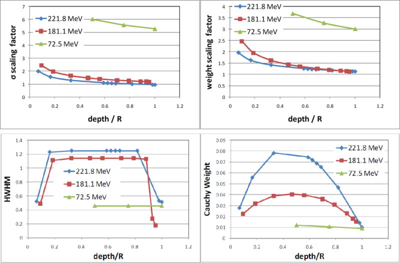
Top plots: scaling factors as power functions of relative depth normalized by beam ranges. Factor values for three energies are displayed to illustrate the extent of the adjustments. Soukup’s formula for nuclear interaction correction was adapted for our specific proton scanning beam line by using these scaling factors. Bottom plots: half width at half maximum (HWHM) and weight of the modified Cauchy-Lorentz component at various depths for three energies.

2.6 Field size effect

We studied field size effects by arranging scanning spots with equal spacing and weights to form square fields with different sizes. We used 5 mm spot spacing. So for field size 2cm×2cm, there are 25 spots, and for 20cm×20cm, there are 1681 spots. The doses measured and calculated at the center of the square fields were plotted as a function of field size, and the dose values were normalized using the values at the field size 10×10 cm² to determine field size factors (FSF).

3. Results

In Figure 3, measured single-spot profiles (markers), and the corresponding computed profiles modeled using the two Gaussian components and Cauchy-Lorentz component (solid lines) and only the two Gaussian components (dashed lines) are shown. The semi-log plots of the lateral profiles show that the impact of long-range scattering, which may be insufficiently modeled using the two Gaussian components, increases as the beam energy increases. Along the depth direction, the discrepancy between the calculations performed with and without the Cauchy-Lorentz component is greater at the intermediate depths than near shallow and deep depths.

Figure 3.

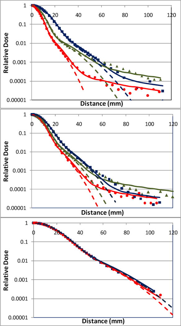
Lateral profiles of individual scanning spots modeled at various depths using the double Gaussian functions and Cauchy-Lorentz component (solid lines) and double Gaussian functions only (dashed lines). The measured lateral profiles at shallow, medium and deep depths are indicated by circle, triangle and square markers respectively. In the top plot (221.8 MeV), red circles, green triangles, blue squares and the corresponding solid and dashed lines correspond to depths 2, 19, and 30 cm, respectively. In the middle plot (181.1 MeV), red circles, green triangles, blue squares and the corresponding lines correspond to depths 2, 10, and 20 cm, respectively. In the bottom plot (72.5 MeV), red circles, blue squares and the corresponding solid and dashed lines represent depths 2 and 4cm, respectively.

The discrepancy caused by switching the Cauchy-Lorentz component on and off can accumulate over a large number of scanning spots. To evaluate this cumulative effect, the FSF calculated for 221.8 MeV with and without the Cauchy-Lorentz component are plotted in Figure 4 as a function of field size for various depths alongside the measured values. The relative differences between the calculation and measurement were also plotted as the function of field size (Figure 5). Without the Cauchy-Lorentz component, the difference between the calculated and measured FSF was 7.9% at the depth 15 cm for proton energy 221.8 MeV and was around 4% at the depth 10 cm for 181.1 MeV. In comparison, the difference near the shallowest and deepest depths generally remained within 3% for the above energies. The addition of the Cauchy-Lorentz component greatly improved the accuracy of FSF calculation for all of the energies tested, and the differences between the prediction of the model and measurement were generally confined within 2%. For proton energy 72.5 MeV, the differences were within 2% regardless of whether the Cauchy-Lorentz component was used.

Figure 4.

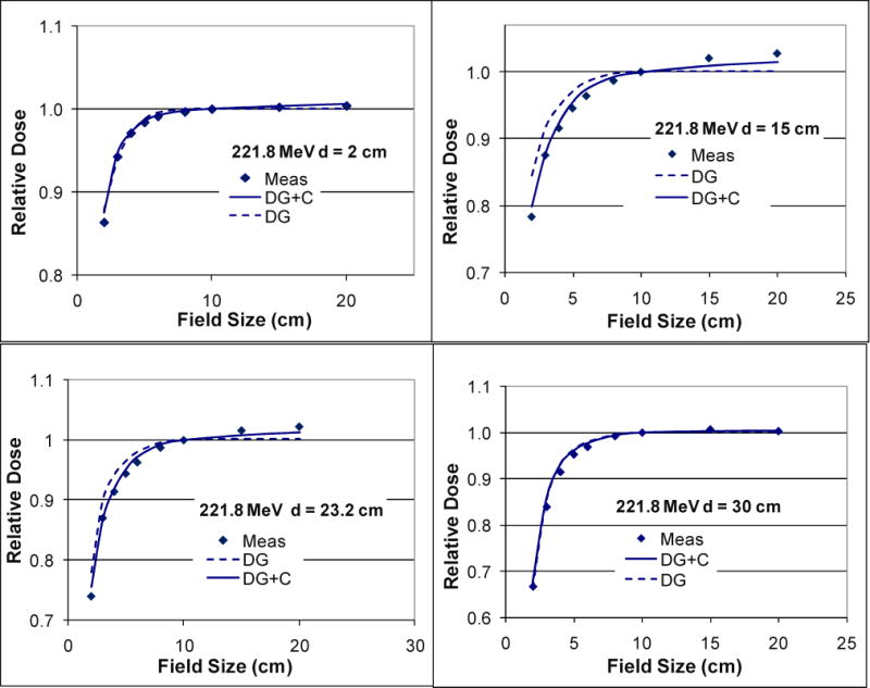
Doses calculated and measured (Meas) for 221.8 MeV at the centers of a series of square fields with different sizes normalized to the central-axis dose of the field size 10×10 cm² showing the field size effects in the spot scanning proton therapy. Compared with the measurements (squares), these field size effects were more accurately modeled with the two Gaussian functions and Cauchy-Lorentz component (DG+C; solid lines) than with the two Gaussian functions only (DG; dashed lines) at the medium depths (15 and 23.2 cm).

Figure 5.

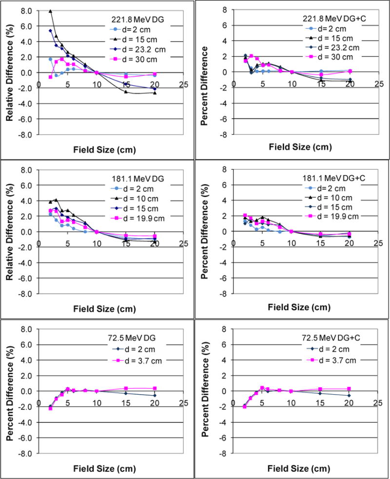
Percentage difference between the measured and calculated dose for three energies at the central axis under a series of square field sizes. The graphs in the left column show relative differences of calculations using two Gaussians (DG) only with measurements at various depths d. The graphs in the right column show relative differences of calculations using two Gaussian functions and Cauchy-Lorentz component (DG+C) at various values of d.

We validated our dose calculation algorithm implementation using patient-specific quality assurance data measured in water phantoms for three single-field uniform-dose (SFUD) treatment plans for prostate cancer patients and one IMPT treatment plan for a head and neck cancer patient. Figure 6 shows the depth dose distribution for one of the prostate cancer cases with a maximum beam energy around 200 MeV. The scanning patterns were created using an early version of our clinical TPS (Eclipse v8.1) with a single Gaussian function for in-air lateral profiles to presumably produce uniform dose distributions in the target region. Notice that the dose value dips near the end of the beam range because the field size narrowed near the distal ends to conform to the round shape of the prostate, and the calibration factors obtained under the broad beam settings were no longer accurate for smaller fields. (The scanning dose calculation model in the clinical TPS has been updated with a double-Gaussian function for in-air lateral profiles since the prostate cancer treatment plan was generated.) Computation using the model developed in this work with the two Gaussian components and Cauchy-Lorentz component showed better agreement with the measured results in both the longitudinal and lateral direction in all of the prostate treatment plans compared with the computation using the two Gaussian components only. In particular, the computed results closely followed the non-uniform dose pattern measured along the beam’s central axis, particularly near the end of the beam range. In addition to accurately predicting the absolute dose along the central axis, gamma index analysis showed that at least 99.8% of the dose pixels passed the 2% dose and 2mm distance matching criteria in all transverse planes at various depths measured using a 2D ionization chamber array for all of the prostate cancer treatment plans. For the multi-field optimized IMPT treatment plan with a maximum beam energy around 145 MeV for the head and neck cancer case, the dose distribution was validated along different longitudinal paths of each field; 2D iso-dose contours were compared in the planes perpendicular to the beam direction measured at various depths. Figure 7 shows the validation of the depth dose calculation for highly nonuniform dose distributions of each field. Gamma index analysis of the 2D iso-dose distributions showed that at least 99.4% of the dose pixels passed 2% and 2-mm matching criteria. Figure 8 shows a comparison of the iso-dose contour for all depths measured in solid water for the first field of the head and neck treatment plan. For this case, no notable difference was observed between calculations with and without the Cauchy-Lorentz component.

Figure 6.

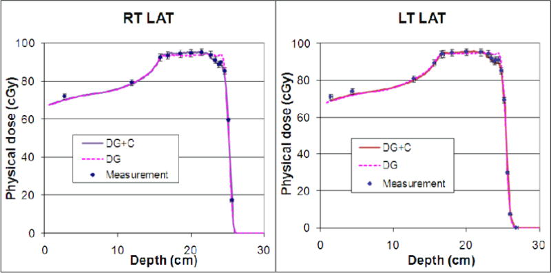
Verification of the in-house dose calculation using two Gaussian functions and Cauchy-Lorentz component (DG+C; solid lines) and two Gaussian functions only (DG; dashed lines) in the patient-specific quality assurance measurements (Meas; squares) on a single field uniform dose proton treatment for one of the prostate cancer patients. Notice that the dose dips near the distal ends of both fields (Right Lateral or RT LAT, and Left Lateral or LT LAT) because of insufficient field size effect modeling at the time of treatment planning. The addition of the Cauchy-Lorentz component improved the modeling accuracy of this effect.

Figure 7.

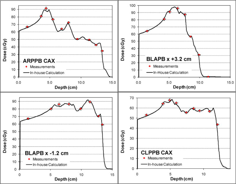
Depth dose profiles measured (squares) and calculated (solid lines) at the central axis (CAX) and positions off the central axis in a three-field IMPT treatment plan for a patient with head-and-neck cancer. Three fields are labeled by ARPPB, BLAPB and CLPPB.

Figure 8.

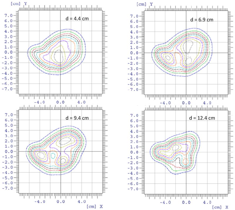
Comparison of the lateral isodose contours measured using 2D ion chamber arrays (solid lines) and the isodose contours calculated by the in-house dose engine (dashed lines) at four different depths for the first scanning field in the head-and-neck IMPT plan.

4. Discussions

We have developed and validated a pencil beam dose calculation algorithm for spot scanning proton beam therapy. It is demonstrated that low dose halos in single-spot profiles in water can be adequately modeled with the addition of a modified Cauchy-Lorentz distribution function to a double Gaussian function. The proposed algorithm could provide the community a valid, validated and systematic approach to correctly model the pencil beam data.

As an increasing number of proton therapy centers under construction or being planned are adopting the spot scanning technique, the issue of dose calculation accuracy will continue to draw great interest. Researchers have increasingly focused their attention on the long-range scattering effect, which may not be fully modeled by Gaussian functions based on single spot measurement data (Ciangaru et al. 2009, Sawakuchi et al. 2010). To our knowledge, this study is the first to exploit a function other than Gaussian function to describe the long-range scattering effects in a proton pencil-beam algorithm. We demonstrated that the modified Cauchy-Lorentz component improved modeling of the field size effects in spot scanning beams that are closely related to the accurate description of single scanning spots. All of the modeling parameters in our study can be derived based on measurement data at a few selected energies and depths for a given energy. We validated the accuracy of the dose calculation algorithm on the basis of good agreement seen between the predicted dose distributions for patient-specific treatment field verification plans and the corresponding measured data. This general method can be implemented in other TPS to improve dose calculation accuracy and reduce commissioning efforts. Considering that commissioning data in our center were generated using Monte Carlo simulations validated using measurements, the procedure based solely on measured data can be especially favorable to centers without the Monte Carlo computation capability.

We developed a modified version of Soukup’s formula to describe the weight and width of the second Gaussian function and added a Cauchy-Lorentz component to better model the longrange effects that cannot be taken into account by using Gaussian functions alone. Soukup’s original work was based solely on Monte Carlo simulations, and few measurement data were available at that time. Now, with more measured data becoming available in our center (Anand et al. 2011), it is necessary to verify and adapt the original formulism for our specific beam-line design.

Although large relative dose errors may occur without consideration of the Cauchy-Lorentz component, the errors were noteworthy only for very high energies and mostly at medium depths. In the PTC-H, the highest beam energy required in many clinical treatment planning tasks, including those for prostate cancer, is about 200 MeV. In that energy range, the importance of the Cauchy-Lorentz component may not always be manifested. However, at medium depths where a scanning spot are not dominated by the peak dose of another spot, such as in cases of IMPT or with distal edge tracking (DET), the Cauchy-Lorentz component may become important.

The handling of field size dependence by the initial version of our clinical TPS, with a single Gaussian function for in-air profiles, was unsatisfactory, which can be noted in the above described prostate cancer treatment plans designed using that version of the TPS. Currently, the issue has been greatly improved since an additional Gaussian component was added to in-air fluence modeling. However, tremendous efforts had to be devoted to determine the parameters for the second Gaussian by a “trial and error” process. In addition, the center’s physics team had to commission separate sets of modeling parameters for large and small field sizes (Zhu et al. 2011). To fit the measurement data, especially the field size effects, the in-air Gaussian components had to be “fudged.” Consequently, the corresponding in-air profiles may deviate from the actual profiles. Intrinsically, the fudged factors do not reflect the underlying physics of the long-range scattering interactions and thus may appear to be somewhat artificial. We have shown that our proposed dose algorithm models the field size effect accurately without requiring any unphysical fudging factors, thus reducing commissioning efforts. A second Gaussian in air may also be configured in our model and the parameters could also be fitted in the similar way as other parameters used in our model. In practice, we found it was not necessary to include second Gaussian in air for our model. For other system, the second Gaussian in air may be added if it is necessary.

5. Conclusion

We studied single scanning spot modeling and its impact on field size effects on dose output and dose calculation accuracy for proton therapy. We also developed and implemented a dose calculation algorithm based on the previously published proton pencil-beam algorithms for spot scanning proton beams. The dose calculation accuracy in IMPT treatment planning may be improved by precisely modeling the low-dose halos of single scanning spots. We explained the formulation and necessary measurement data for adaptation of Soukup’s nuclear interaction correction for specific scanning proton beam lines. We proposed using a third component in addition to two Gaussian components based on the Cauchy-Lorentz function to improve the modeling accuracy of lateral dose profiles for high-energy scanning spots. This may be especially important to improving the dose accuracy with intensity modulated and distal edge tracking techniques or similar situations at high proton beam energies.

References

- Anand A, Sahoo N, Zhu XR, Titt U, Sawakuchi G, Li Y, Poenisch F, Amos R, Suzuki K, Ciangaru G, Mohan R, Gillin M. Joint AAPM/COMP Meeting. Vancouver, BC: 2011. Scanned Proton Pencil Beam’s Lateral Profile Library to Describe the Spot Dose Characteristics. [Google Scholar]
- Ares C, Khan S, Macartain aM, Heuberger J, Goitein G, Gruber G, Lutters G, Hug EB, Bodis S, Lomax aJ. POSTOPERATIVE PROTON RADIOTHERAPY FOR LOCALIZED AND LOCOREGIONAL BREAST CANCER: POTENTIAL FOR CLINICALLY RELEVANT IMPROVEMENTS? International Journal of Radiation Oncology Biology Physics. 2010;76:685–697. doi: 10.1016/j.ijrobp.2009.02.062. [DOI] [PubMed] [Google Scholar]
- Bortfeld T. An analytical approximation of the Bragg curve for therapeutic proton beams. Medical Physics. 1997;24:2024–2033. doi: 10.1118/1.598116. [DOI] [PubMed] [Google Scholar]
- Ciangaru G, Sahoo N, Zhu XR, Sawakuchi GO, Gillin MT. Computation of doses for large-angle Coulomb scattering of proton pencil beams. Physics in Medicine and Biology. 2009;54:7285–7300. doi: 10.1088/0031-9155/54/24/003. [DOI] [PubMed] [Google Scholar]
- Deasy JO. A proton dose calculation algorithm for conformal therapy simulations based on Moliere’s theory of lateral deflections. Medical Physics. 1998;25:476–483. doi: 10.1118/1.598222. [DOI] [PubMed] [Google Scholar]
- Gillin MT, Sahoo N, Bues M, Ciangaru G, Sawakuchi G, Poenisch F, Arjomandy B, Martin C, Titt U, Suzuki K, Smith aR, Zhu XR. Commissioning of the discrete spot scanning proton beam delivery system at the University of Texas MD Anderson Cancer Center, Proton Therapy Center, Houston. Medical Physics. 2010;37:154–163. doi: 10.1118/1.3259742. [DOI] [PMC free article] [PubMed] [Google Scholar]
- Gottschalk B. Passive beam spreading in proton radiation therapy. 2004 http://huhepl.harvard.edu/~gottschalk.
- Grevillot L, Bertrand D, Dessy F, Freud N, Sarrut D. A Monte Carlo pencil beam scanning model for proton treatment plan simulation using GATE/GEANT4. Physics in Medicine and Biology. 2011;56:17. doi: 10.1088/0031-9155/56/16/008. [DOI] [PubMed] [Google Scholar]
- Hong L, Goitein M, Bucciolini M, Comiskey R, Gottschalk B, Rosenthal S, Serago C, Urie M. A pencil beam algorithm for proton dose calculations. Physics in Medicine and Biology. 1996;41:1305–1330. doi: 10.1088/0031-9155/41/8/005. [DOI] [PubMed] [Google Scholar]
- Inaniwa T, Furukawa T, Nagano A, Sato S, Saotome N, Noda K, Kanai T. Field-size effect of physical doses in carbon-ion scanning using range shifter plates. Medical Physics. 2009;36:2889–2897. doi: 10.1118/1.3140586. [DOI] [PubMed] [Google Scholar]
- Lomax aJ, Bortfeld T, Goitein G, Debus J, Dykstra C, Tercier PA, Coucke PA, Mirimanoff RO. A treatment planning inter-comparison of proton and intensity modulated photon radiotherapy. Radiotherapy and Oncology. 1999;51:257–271. doi: 10.1016/s0167-8140(99)00036-5. [DOI] [PubMed] [Google Scholar]
- Merchant TE, Hua CH, Shukla H, Ying XF, Nill S, Oelfke U. Proton versus photon radiotherapy for common pediatric brain tumors: Comparison of models of dose characteristics and their relationship to cognitive function. Pediatric Blood & Cancer. 2008;51:110–117. doi: 10.1002/pbc.21530. [DOI] [PubMed] [Google Scholar]
- Muzik J, Soukup M, Alber M. Comparison of fixed-beam IMRT, helical tomotherapy, and IMPT for selected cases. Medical Physics. 2008;35:1580–1592. doi: 10.1118/1.2890085. [DOI] [PubMed] [Google Scholar]
- Pedroni E, Scheib S, Bohringer T, Coray A, Grossmann M, Lin S, Lomax A. Experimental characterization and physical modelling of the dose distribution of scanned proton pencil beams. Physics in Medicine and Biology. 2005;50:541–561. doi: 10.1088/0031-9155/50/3/011. [DOI] [PubMed] [Google Scholar]
- Petti PL. Differential-pencil-beam dose calculations for charged-particles. Medical Physics. 1992;19:137–149. doi: 10.1118/1.596887. [DOI] [PubMed] [Google Scholar]
- Russell KR, Isacsson U, Saxner M, Ahnesjo A, Montelius A, Grusell E, Dahlgren CV, Lorin S, Glimelius B. Implementation of pencil kernel and depth penetration algorithms for treatment planning of proton beams. Physics in Medicine and Biology. 2000;45:9–27. doi: 10.1088/0031-9155/45/1/302. [DOI] [PubMed] [Google Scholar]
- Sawakuchi GO, Zhu XR, Poenisch F, Suzuki K, Ciangaru G, Titt U, Anand A, Mohan R, Gillin MT, Sahoo N. Experimental characterization of the low-dose envelope of spot scanning proton beams. Physics in Medicine and Biology. 2010;55:3467–3478. doi: 10.1088/0031-9155/55/12/013. [DOI] [PubMed] [Google Scholar]
- Schaffner B. Proton dose calculation based on in-air fluence measurements. Physics in Medicine and Biology. 2008;53:1545–1562. doi: 10.1088/0031-9155/53/6/003. [DOI] [PubMed] [Google Scholar]
- Schaffner B, Pedroni E, Lomax A. Dose calculation models for proton treatment planning using a dynamic beam delivery system: an attempt to include density heterogeneity effects in the analytical dose calculation. Physics in Medicine and Biology. 1999;44:27–41. doi: 10.1088/0031-9155/44/1/004. [DOI] [PubMed] [Google Scholar]
- Soukup M, Fippel M, Alber M. A pencil beam algorithm for intensity modulated proton therapy derived from Monte Carlo simulations. Physics in Medicine and Biology. 2005;50:5089–5104. doi: 10.1088/0031-9155/50/21/010. [DOI] [PubMed] [Google Scholar]
- Ulmer W, Schaffner B. Foundation of an analytical proton beamlet model for inclusion in a general proton dose calculation system. Radiation Physics and Chemistry. 2011;80:378–389. [Google Scholar]
- Weber DC, Trofimov aV, Delaney TF, Bortfeld T. A treatment planning comparison of intensity modulated photon and proton therapy for paraspinal sarcomas. International Journal of Radiation Oncology Biology Physics. 2004;58:1596–1606. doi: 10.1016/j.ijrobp.2003.11.028. [DOI] [PubMed] [Google Scholar]
- Zhang X, Li Y, Pan X, Li X, Mohan R, Komaki R, Cox JD, Chang JY. Intensity-Modulated Proton Therapy Reduces the Dose to Normal Tissue Compared With Intensity-Modulated Radiation Therapy or Passive Scattering Proton Therapy and Enables Individualized Radical Radiotherapy for Extensive Stage IIIB Non-Small-Cell Lung Cancer: A Virtual Clinical Study. International Journal of Radiation Oncology Biology Physics. 2010:77, 357–366. doi: 10.1016/j.ijrobp.2009.04.028. [DOI] [PMC free article] [PubMed] [Google Scholar]
- Zhang X, Liu W, Li Y, Li X, Quan M, Mohan R, Anand A, Sahoo N, Gillin M, Zhu XR. Parameterization of multiple Bragg curves for scanning proton beams using simultaneous fitting of multiple curves. Physics in Medicine and Biology. 2011;56:7725–7735. doi: 10.1088/0031-9155/56/24/003. [DOI] [PubMed] [Google Scholar]
- Zhu XR, Poenisch F, Lii M, Sawakuchi G, Titt U, Ciangaru G, Bues M, Zhang X, Song X, Suzuki K, Gillin M, Sahoo N. Commisioning dose models for spot scanning proton beams in water. Medical Physics. 2011 doi: 10.1118/1.4798229. (submitted) [DOI] [PMC free article] [PubMed] [Google Scholar]