Analyzing LC-MS/MS data by spectral count and ion abundance: two case studies

Abstract

In comparative proteomics studies, LC-MS/MS data is generally quantified using one or both of two measures: the spectral count, derived from the identification of MS/MS spectra, or some measure of ion abundance derived from the LC-MS data. Here we contrast the performance of these measures and show that ion abundance is the more sensitive. We also examine how the conclusions of a comparative analysis are influenced by the manner in which the LC-MS/MS data is ‘rolled up’ to the protein level, and show that divergent conclusions obtained using different rollups can be informative. Our analysis is based on two publicly available reference data sets, BIATECH-54 and CPTAC, which were developed for the purpose of assessing methods used in label-free differential proteomic studies. We find that the use of the ion abundance measure reveals properties of both data sets not readily apparent using the spectral count.

1. INTRODUCTION

Comparative proteomics studies aim to discern differences in protein content and abundance between case and control samples. Tandem liquid-chromatography mass-spectrometry (LC-MS/MS) experiments are performed routinely in carrying out such studies and may employ labeled or unlabeled samples. Our focus here will be on the analysis of data from unlabeled experiments.

Preparatory to an LC-MS/MS experiment, a protein sample is digested using trypsin or another proteolytic enzyme. In LC-MS, a reverse phase liquid chromatography (LC) column is typically used to separate the resulting peptide ‘species’ based on their hydrophobicity, and an MS spectrum, or scan, is taken of them periodically as they elute. The collection of scans from a single experiment may be viewed as a three-dimensional landscape of peaks located in elution time (t) and mass/charge (m/z) space. We refer to the recent reviews [6] and [8] for a more detailed discussion of LC-MS/MS experimental and analytical procedures.

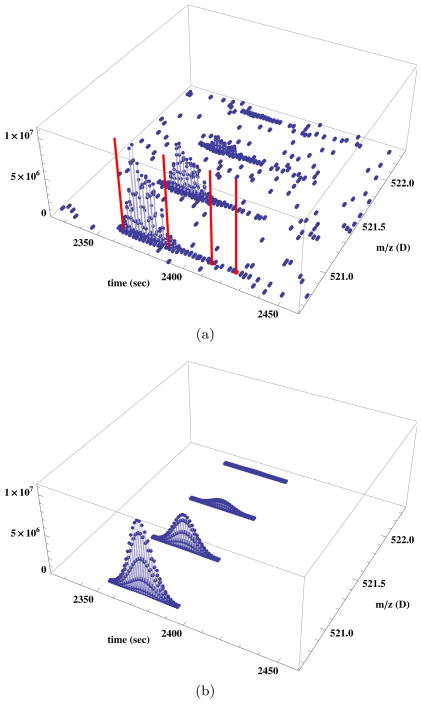
The peaks associated with a single species form a characteristic group, or ‘feature’, in LC-MS space. An example of such a feature is shown in Figure 1(a). Each peak in the group collects ions of one or more isotopic forms of the species. The relative amplitude of the peaks measures the relative abundance of the isotopic forms. A number of software packages have been developed to detect and quantify LC-MS features including MapQuant [19], MaxQuant [4], Sahale [25], Serac [28], SpecArray [20], and SuperHirn [26].

Figure 1. An LC-MS feature and its quantification.

(a) The LC-MS feature associated with the species GGALDFADFK+2 identified in file 54ProtMix 1ug 051207 SampA1 01.mzXML of the BIATECH-54 data set [18]. Red lines indicate the location at which MS/MS spectra were taken, and later identified as originating with this species by X!Tandem. (b) The fit to this feature made by Sahale [25].

In tandem MS (MS/MS), selected LC-MS peaks are interrogated by a collision-induced dissociation (CID) and a second MS scan recorded. Figure 1(a) displays the (t, m/z) locations (shown in red) of four MS/MS scans sampled from the LC-MS feature. MS/MS spectra are matched against a protein database to determine the species from which they likely originated. In the simplest case, the species is one of the amino acid sequences generated by an in silico digest of the protein database, e.g., by trypsin. The search space, however, is usually expanded beyond that of the in silico digest to include, for example, species with missed or non-tryptic cleavages, and species with altered mass due to anticipated chemical modifications of specific amino acids. Algorithms to perform this search are implemented by software packages including MyriMatch [34], Sequest [10], and X!Tandem [5]. Following identification, each spectrum-to-species match is assigned an instrument-independent quality score, typically either a PeptideProphet score [17], or a false discovery rate (FDR) calculated on the basis of hits against decoy proteins in the database searched [15].

In the analysis of LC-MS/MS data, the relative abundance of species in a sample is generally quantified by either or both of two measures: the spectral count (see, e.g, [2, 21, 22, 37]), which is the number of MS/MS spectra identified as arising from the species, or some measure of the species’ ion abundance derived from an analysis of its feature signature in LC-MS space (see, e.g., [1, 14, 19, 28]). For example, the spectral count associated with the species giving rise to the feature in Figure 1(a) is four, and one possible measure of the species’ ion abundance is the volume of the peaks fitted to its feature, as shown in Figure 1(b). Recently, the ion abundance of MS/MS spectra has been introduced as one component of an alternative quantitative measure [12]; we do not consider this measure of abundance in this work.

We note that although it is the species that is observed directly in a LC-MS/MS experiment, and for which such experiments yield quantitative data, the goal of comparative proteomics studies is to identify and quantify the proteins. In particular, the data available for species must be ‘rolled up’ to the protein level. To date, no systematic research has addressed how best to infer protein quantity from the species quantities [30], although some statistical discussion on this topic is provided by [3] for ion abundance and [23] for spectral count. A common approach is to average the quantitative measure used (i.e., spectral count or ion abundance) for all species belonging to a particular protein and then to use the result as a surrogate measure for the abundance of the protein in a statistical test. Other investigations infer relative protein abundance directly from the abundance of species, or from the abundance of species data rolled up to some intermediate level, using a variety of methods. For methods based on spectral counts, see APEX [22], emPAI [13], QSpec [2], SASPECT [36, 35] and Spectral Index [11]. For statistical models of protein rollup based on ion abundances, see [3, 16]. The recent review [27] provides additional perspective.

In this paper we contrast the performance of the spectral count and ion abundance in quantifying LC-MS/MS data. We also consider the effect of various levels of data aggregation—from the species level to the protein level—prior to, or simultaneously with, the analysis of the relative abundance of proteins. We conclude that ion abundance, coupled with an appropriate rollup procedure, is the more sensitive measure for use in comparative analysis. Our findings are based on detailed examinations of two publicly available reference data sets, BIATECH-54 [18] and CPTAC [29], which were developed to assess methods of protein identification and quantification in LC-MS/MS experiments. The use of the ion abundance measure reveals characteristics of both the BIATECH-54 and CPTAC data sets not readily apparent by the use of the spectral count.

2. METHODS

2.1 Quantification

We used Sahale [25] to determine the spectral count and ion abundance of species identified by X!Tandem in the BIATECH-54 and CPTAC data. Briefly, Sahale searches for LC-MS features in the vicinity of the (t, m/z) location of those species identified by MS/MS satisfying a specified quality threshold, either a PeptideProphet score or false discovery rate (FDR). The species’ spectral count is the number of MS/MS identifications of that species satisfying the threshold. The species’ ion abundance is determined by fitting the corresponding feature to the model f ≡ f(t, m),

$$f=A\stackrel{\text{model}\text{in}t}{\overbrace{exp\left[-\frac{{(t-\mu )}^2}{2{\sigma }^2}\right]}}\stackrel{\text{model}\text{in}m/z}{\overbrace{\left(\sum _{k=0}^{N-1}\frac{{\lambda }^k}{k!}{e}^{-\lambda }exp\left[-\frac{{(m-{\zeta }_k)}^2}{2{\rho }^2}\right]\right)}},$$ (1)

and taking the total volume under the fitted surface,

$$2\pi A\sigma \rho \sum _{k=0}^{N-1}\frac{{\lambda }^k}{k!}{e}^{-\lambda },$$

as a surrogate measure of ion abundance. f(t, m) is the product of a simple Gaussian in the chromatographic (t) coordinate and a series of N Gaussians with Poisson-distributed peak amplitudes in the m/z (m) coordinate. In Equation (1), A is the amplitude. μ is the coordinate of the peak of the time Gaussian and σ is its standard deviation. For the function in m/z, N is the number of isotopic peaks modeled, ζ_k = ζ₀+kδ is the m/z location of the kth peak, ζ₀ is the co-ordinate of the first Poisson-distributed peak, k is the peak number, δ is the inter-peak spacing, λ is the Poisson parameter, and ρ is the standard deviation of the Gaussians. Sahale fits Equation (1) to data by least squares using the Levenberg-Marquardt minimization algorithm. Figure 1(b) shows the fit determined by Sahale to the feature shown in Figure 1(a).

Sahale returns the spectral count and ion abundance for every species for which at least one MS/MS identification exists satisfying the quality threshold specified. Because Sahale quantifies LC-MS features guided by MS/MS identifications, and not all the corresponding ion abundance quantifications are determined successfully, the number of species quantified by ion abundance is less than or equal to the number quantified by spectral count.

2.2 Rollup and significance analysis

The data collected in an LC-MS/MS experiment quantifies the species. To determine the relative abundance of proteins, a statistical analysis might use the quantitative data for species directly, or will first aggregate the species-level quantitative data to some higher rollup level.

A species as we’ve defined the term is the identity associated with a feature in LC-MS space by a search of a protein database, e.g., by X!Tandem. A species is characterized by three attributes: its primary amino acid sequence, any chemical modifications to its amino acids, and its charge state. The nomenclature DEDTQAM[147.035]PFR+2, for example, identifies a species with the primary amino acid sequence DEDTQAMPFR containing an oxidized methionine at position 7 with a net mass of 147.035 Daltons (D) and carrying a charge of +2 induced by the LC-MS instrument. A like species with charge +3, DEDTQAM[147.035]PFR+3, might be identified in the same experiment. Other species might be identified in the experiment with the same primary amino acid sequence but without the modification to methionine, i.e., DEDTQAMPFR+2 and DEDTQAMPFR+3. In general, these species variants, all of which have the same primary amino acid sequence, will correspond to widely-separated features in LC-MS space.

The key point is that as a result of biological processes and the action of the LC-MS instrument, a short segment of a protein’s primary amino acid sequence may present itself as any number of species — and corresponding features — in an LC-MS/MS experiment.

We define three levels of rollup of LC-MS/MS data.

• Species: The base rollup level.

• Peptide: The collection of all species with the same primary amino acid sequence. The peptide DEDTQAMPFR, for example, refers to the species DEDTQAMPFR+2, DEDTQAMPFR+3, DEDTQAM[147.035]PFR+2, etc.

• Protein: The collection of all species that by virtue of their primary amino acid sequence possibly originated from a particular protein.

Where it is convenient, we refer to the rollup level by a single-letter abbreviation: species (s), peptide (p), or protein (P). Note that we use the term ‘protein’ to refer to both a rollup level and to the biological entity; the meaning will be clear from the context.

We assigned to the higher rollup entities — the peptides and proteins — a spectral count and ion abundance by a simple sum. For example, we computed the spectral count (ion abundance) for a particular peptide to be the sum of the spectral counts (ion abundances) for all species that are elements of the peptide.

To test for proteins present in differing abundance, we computed a statistic, τ_r, that integrates the evidence of difference, w, measured for each of a protein’s K constituent elements identified at rollup level r,

$${\tau }_r={\tau }_r(w_k,k=1,K)=\frac{1}{K}\sum _{k=1}^K{w}_k.$$ (2)

Note that w_k is w for the k’th element of a protein at rollup level r. τ_r is simply the mean of the w’s measured for a protein’s r-level rollup elements.

For the element-level measure of difference, w, we employed a zero-centered and scaled version of the Wilcoxon test statistic, W, which is the sum of ranks of observations in the case group in a case-control comparison. W naturally falls in the range

$$[W_{min},W_{max}]=\left[\frac{n}{2}(n+1),\frac{n}{2}(n+2m+1)\right],$$

where n and m are the number of case and control observations, respectively, being compared. In our analysis, we took the ‘observations’ to correspond to the biological replicates. We define w as

$$w=\frac{2}{W_{max}-W_{min}}\left[W-\left(\frac{W_{max}+W_{min}}{2}\right)\right].$$ (3)

Thus defined, w ∈ [−1, 1]. Henceforth, for brevity, we refer to the scaled and re-centered Wilcoxon statistic w simply as the Wilcoxon. As a consequence of the definition of w, τ_r, defined in Equation (2), falls in the range [−1, 1] independently of K. Note that at the protein level of rollup, K = 1 and τ_P = w, where w is the Wilcoxon computed for the protein at the protein level of rollup.

We computed τ_r using both the spectral count and ion abundance measures for all elements at the species, peptide and protein rollup levels. To derive p-values, we computed a null distribution for τ_r by repeatedly permuting the labels of the case and control samples (1,500x in both the BIATECH-54 and CPTAC studies).

Our aim is to contrast quantification by spectral count and ion abundance as transparently as possible. This demands that the statistical summaries we employ must be comparable and based on the same concepts. The statistic τ_r is simply the average of Wilcoxon test statistics for a protein’s constituent elements at a given rollup level, computed in the same way at each level using the spectral count or the ion abundance.

3. CASE STUDIES

3.1 BIATECH-54

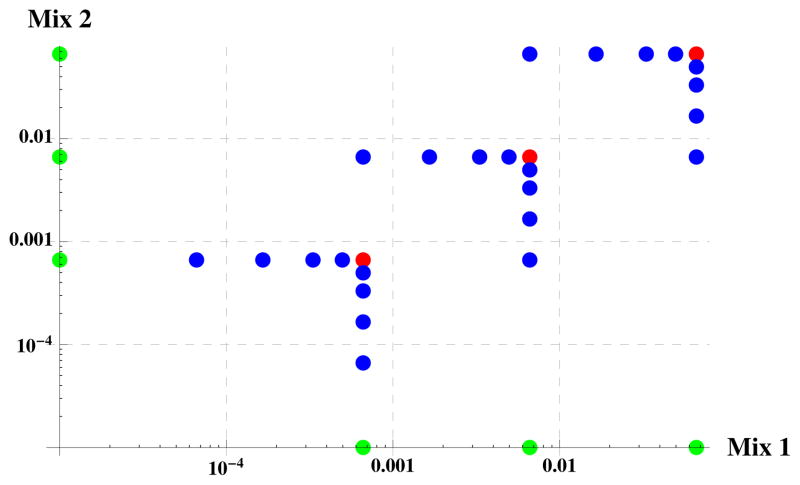
We describe first our analysis of the LC-MS/MS data set measuring the two reference samples, Mix 1 and Mix 2, of the BIATECH-54 set (Kolker et al. [18]). The BIATECH-54 mixtures were developed to assess methods of protein identification and quantification in LC-MS/MS experiments. Mix 1 and Mix 2 combine 54 proteins at different concentrations; their exact compositions are documented in Table 1 of [18] and represented graphically in Figure 2. To mimic biological replicates, Kolker et al. prepared six (6) replicate samples of Mix 1 and Mix 2 and digested each independently with trypsin. The twelve (12) samples were then each subject to LC-MS/MS analysis twice; these are the technical replicates.

Figure 2. BIATECH-54 study design.

The log milligram (mg) fractional abundances (mg of protein/total mg in the sample) of proteins in Mix 1 and Mix 2 of the BIATECH-54 set. The blue, green and red points represent 1, 2 and 6 proteins, respectively (54 total). Those proteins for which zero mg was included in either sample are shown on the axes.

The BIATECH-54 data set was obtained from the authors as a collection of 24 files in .mzXML format [18]. In this collection, files corresponding to the Mix 1 samples are designated ‘A’ and Mix 2 samples designated ‘B’.

We searched the MS/MS spectra of the data set using X!Tandem [5] against a protein database containing the primary amino acid sequences of the proteins of yeast along with those of the BIATECH-54 and potential contaminating proteins. To support estimation of the false discovery rate, decoy protein sequences, constructed by reversing each of the target protein sequences, were appended to this database [9]. To compensate for drift in the calibration of the LTQ-FT instrument used to collect these data, the precursor matching tolerance was set to an asymmetric window [−10 ppm, +40 ppm]. The search was performed to allow potential oxidation of methionines (Δmass = 15.9949D). Up to two missed tryptic cleavages were permitted.

We conducted separate searches allowing for only fully-tryptic species and for semi-tryptic species. As implemented by X!Tandem, the latter are species constrained to have a tryptic terminus on at least one end. We chose to analyze the results obtained from both the fully- and semi-tryptic searches because it is not uncommon in practice to do one or the other. Though usually not stated explicitly, the rationale for using a semi-tryptic search is that such species are likely to be present in samples, e.g., due to the activity of contaminating proteolytic enzymes, and ignoring such species would leave potentially useful quantitative data ‘on the table’.

The BIATECH-54 data was quantified by spectral count and ion abundance using Sahale [25]. The FDR threshold parameter set for Sahale was selected to be 0.001 (see Section 2.1). Species not observed or quantified in at least three (3 of 12) of the Mix 1 samples or three (3 of 12) of the Mix 2 samples were filtered out, as were uninformative species in the ion abundance data for which the ion abundances are effectively zero or are missing for all samples. The spectral counts and ion abundances for the species remaining were then rolled up to the peptide and protein levels (see Section 2.2). The resulting six data sets — the spectral counts and ion abundances across the three rollup levels — were then normalized by sample to make the data comparable across samples. The spectral counts were normalized by the total spectral count, and ion abundances by the median ion abundance.

As already described, the BIATECH-54 data set includes two technical replicate observations of each of the 12 biological samples measured. The technical replicates were ‘averaged’ to obtain a value for the spectral count and ion abundance for the corresponding biological replicate. The average was computed so that if one of the technical observations was found to be missing, the quantity found for the other was assigned as that for the biological replicate.

Following these preparatory steps, we tested the species, peptide and protein level entities in Mix 1 and Mix 2 for evidence of difference using the statistic τ_r (Equation (2)).

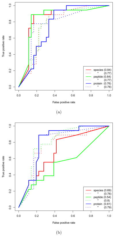
Figure 3, displays ROC curves characterizing the performance of τ_r in correctly characterizing the relative abundance of proteins in the BIATECH-54 samples. Figure 3(a) shows ROC curves determined by analysis of the data searched for fully-tryptic species; Figure 3(b) shows the same results for data searched allowing for semi-tryptic species. The data used to produce both figures was quantified by Sahale with the FDR threshold parameter set to 0.001; qualitatively similar results were obtained with the FDR level set to 0.01 or 0.02 (not shown). The ROC analysis was performed using the ROCR package [32].

Figure 3. ROC comparison of performance.

ROC curves showing the performance of τ_r, computed using the spectral count (dotted) and ion abundance (solid) measures, in characterizing the relative abundance of proteins in Mix 1 and Mix 2 of the BIATECH-54 set across the species, peptide and protein rollup levels. (a) shows the results obtained using the data searched for fully-tryptic species, and (b) for semi-tryptic species. The AUC corresponding to each curve is shown in parenthesis.

In Figure 3(a), we see that at the species and peptide levels the AUC computed using the ion abundance is approximately 9% higher than that obtained using the spectral count; the AUCs are approximately equal at the protein level. The ion abundance at the protein level, however, yields an AUC appreciably less than that at the species and peptide levels. By contrast, the spectral count yields an AUC that is nearly constant across rollup levels.

Using the semi-tryptic data, the relative performance of the spectral count and ion abundance is nearly reversed (Figure 3(b)). Strikingly, the performance of ion abundance at the species and peptide rollup levels is significantly lower than that obtained using the fully-tryptic data whereas the performance at the protein level is nearly the same. With the semi-tryptic data, as with the fully-tryptic, the performance of the spectral count is relatively consistent across rollup levels and approximately equal to the AUCs computed using the fully-tryptic data.

Initially, we were puzzled by these findings, particularly by the disparity of performance, between the fully-tryptic and semi-tryptic data, of ion abundance at the species and peptide levels of rollup. Also confusing is that the performance of ion abundance at the protein level of rollup in the semi-tryptic data ‘recovers’ to that obtained with the fully-tryptic data.

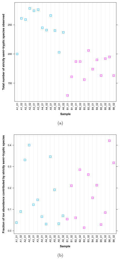
A further examination revealed that these findings reflect an actual difference between the Mix 1 and Mix 2 samples of the BIATECH-54 set not detected using the spectral count. Figure 4(a) shows the total number of strictly semi-tryptic species (i.e., not fully-tryptic) detected in each of the 24 samples of the BIATECH-54 data set. Clearly, strictly semi-tryptic species are observed more frequently in the Mix 1 than in the Mix 2 samples. We believe this fact reflects a difference in the way in which the samples themselves were prepared; a contaminating (non-trypsin) proteolytic enzyme may have been introduced into the Mix 1 samples, or may have been more active in these than in the Mix 2 samples.

Figure 4. Strictly semi-tryptic species content by experiment.

(a) Strictly semi-tryptic species are observed more frequently in the Mix 1 (A) than in the Mix 2 (B) samples of the BIATECH-54 data set, searched to permit the observation of such species. (b) The fraction of the total ion abundance contributed by strictly semi-tryptic species varies little between the Mix 1 and Mix 2 samples.

This difference between the Mix 1 and Mix 2 samples is manifest in the ROC plots for the semi-tryptic data because the structure of τ_r as an average of Wilcoxon statistics makes it sensitive to the contributions made by the additional strictly semi-tryptic species observed in Mix 1. For τ_s, for example, each observation of a strictly semi-tryptic species in Mix 1 that is not in Mix 2 makes an incremental contribution that carries equal weight to the contributions made by species observed in both samples.

Figure 4(b) shows the fraction of ion abundance contributed by the strictly semi-tryptic species in the 24 samples. Despite the fact that more strictly semi-tryptic species are present in Mix 1 than in Mix 2, their relative contribution to the total ion abundance in each sample is nearly equal across samples. This suggests that the ion abundance signal associated with strictly semi-tryptic species is small. It also explains the ‘recovery’ of performance observed in Figure 3(b) for data analyzed at the protein rollup level. Rollup to the protein level ‘hides’ the relatively small contribution made to each protein’s total ion abundance by the low-abundance strictly semi-tryptic species.

It is more difficult to provide a simple explanation for the poor performance seen in Figure 3(b) for the intermediate, peptide level of rollup. The performance is the result of a complex interaction of two factors: the number of species that contribute to the quantification of each peptide; and the relative contribution made by the additional strictly semi-tryptic species observed in the Mix 1 samples to the quantification of each peptide.

Using a semi-tryptic search strategy and the ion abundance measure, we’ve found that the BIATECH-54 samples Mix 1 and Mix 2 differ markedly in their content of strictly semi-tryptic species (Figure 4(a)). We detected this anomaly at the species and peptide levels of rollup, but not at the protein level (Figure 3(b)), using our Wilcoxon rank-sum-based test. The same analysis carried out using the spectral count measure gave no hint of this unanticipated finding. Our analysis suggests not only that the ion abundance is a more sensitive measure of quantification than is the spectral count, but that analysis of LC-MS/MS data at different levels of rollup can be informative.

3.2 CPTAC

In a study conducted by the Clinical Proteomic Technologies for Cancer (CPTAC) consortium, Paulovich et al. [29] introduced a reference data set measuring new performance standards for benchmarking of LC-MS/MS platforms and data analysis methods. These new standards are based on the yeast proteome and the UPS1 (Universal Proteomics Standard Set 1) collection of 48 human source or human sequence recombinant proteins [31]. The CPTAC reference samples and data set therefore provide a more complex and challenging benchmark for LC-MS/MS analysis than does BIATECH-54.

We analzyed a subset of the data collected for the CPTAC study, comparing the trypsin-digested yeast protein lysate samples, designated QC2, with the UPS1 spike-in samples, designated A, B, C, D and E. The composition of these samples is summarized in Table 1, which is excerpted from Section C of [29, Supplementary Information]. The four laboratories participating in the study each collected three technical replicate observations of the QC2, A, B, C, D and E samples for a total of twelve (12) observations of each.

Table 1.

The composition of the CPTAC samples.

Sample	Yeast (ng/μL)	UPS1 (Sigma-48) (fmol/μL)
QC2	60	0
A	60	0.25
B	60	0.74
C	60	2.2
D	60	6.7
E	60	20

The MS/MS spectra were searched using X!Tandem against the same protein database used by the CPTAC authors, which includes both target and decoy (reversed) protein sequences. The precursor matching tolerance was set to [−10 ppm, +10 ppm]. The search was performed to allow for potential oxidation of methionines (Δm = 15.9949D) and carbamidomethylation of cysteines (Δm = 57.0215D). Up to two missed tryptic cleavages were permitted. The search was conducted allowing for only fully-tryptic species.

The CPTAC data was quantified by spectral count and ion abundance using Sahale executed with the FDR threshold parameter set to 0.001. Species not observed or quantified in at least three (3 of 12) of the A, B, C, D or E samples or three (3 of 12) of the QC2 samples were filtered out, as were uninformative species in the ion abundance data for which the ion abundances were effectively zero or were missing for all samples. The data was then rolled up. The spectral counts in each sample were normalized by the total spectral count, and the ion abundances by the median ion abundance.

Following these preparatory steps, we searched for proteins present in differing abundance in the QC2 and A, B, C, D or E samples using the statistic τ_r (Equation (2)) computed at the species, peptide and protein rollup levels. Following the methodology used by Paulovich et al. [29] in the analysis leading to their Table III, we treated the 12 observations of each sample type as biological replicates. Note that because we tested on the rank computed for the QC2 samples, species, peptide or protein elements less abundant in the A–E samples than in QC2 have w > 0. This observation will be important in what follows.

To correct for the effects of multiple hypothesis testing, we converted p-values to false discovery rates using the R package qvalue (see [33]). The numbers of yeast and UPS1 proteins found to be present in greater and lesser abundance in samples A–E relative to QC2 at FDR level 0.05 are shown in Table 2.

Table 2.

The number of yeast and UPS1 proteins found to be present in greater (⇑) and lesser (⇓) abundance in samples A–E relative to QC2 of the CPTAC data at FDR level 0.05.

		sample (vs QC2)	UPS1		yeast		total
			⇑	⇓	⇑	⇓
species	ion abundance	A	0	0	0	0	0
		B	2	0	0	0	2
		C	17	0	0	5	22
		D	35	0	0	12	47
		E	41	0	2	347	390
	spectral count	A	0	0	0	1	1
		B	3	0	0	1	4
		C	21	0	2	7	30
		D	35	0	2	4	41
		E	42	0	27	69	138
peptides	ion abundance	A	0	0	0	0	0
		B	3	0	0	0	3
		C	16	0	0	5	21
		D	35	0	0	18	53
		E	41	0	2	403	446
	spectral count	A	0	0	0	1	1
		B	8	0	1	0	9
		C	23	0	4	9	36
		D	35	0	5	6	46
		E	42	0	20	71	133
proteins	ion abundance	A	0	0	0	0	1
		B	3	0	0	0	3
		C	15	0	0	5	20
		D	35	0	1	31	67
		E	40	0	5	522	567
	spectral count	A	0	0	0	0	0
		B	5	0	0	1	6
		C	24	0	1	8	33
		D	34	0	1	6	41
		E	42	0	11	83	136

Table 2 shows that the performance of the spectral count is somewhat better than ion abundance in correctly characterizing the abundance of the UPS1 proteins in the case samples across rollup levels, particularly at the lower levels of spike-in. However, what stands out in Table 2 is the large number of yeast proteins found to have different abundance in the E and QC2 samples. The number of these apparent false positives is particularly high in the results computed using ion abundance. We sought to understand the origin of these ‘false positives’, initially suspecting some error in the method by which features were quantified by ion abundance.

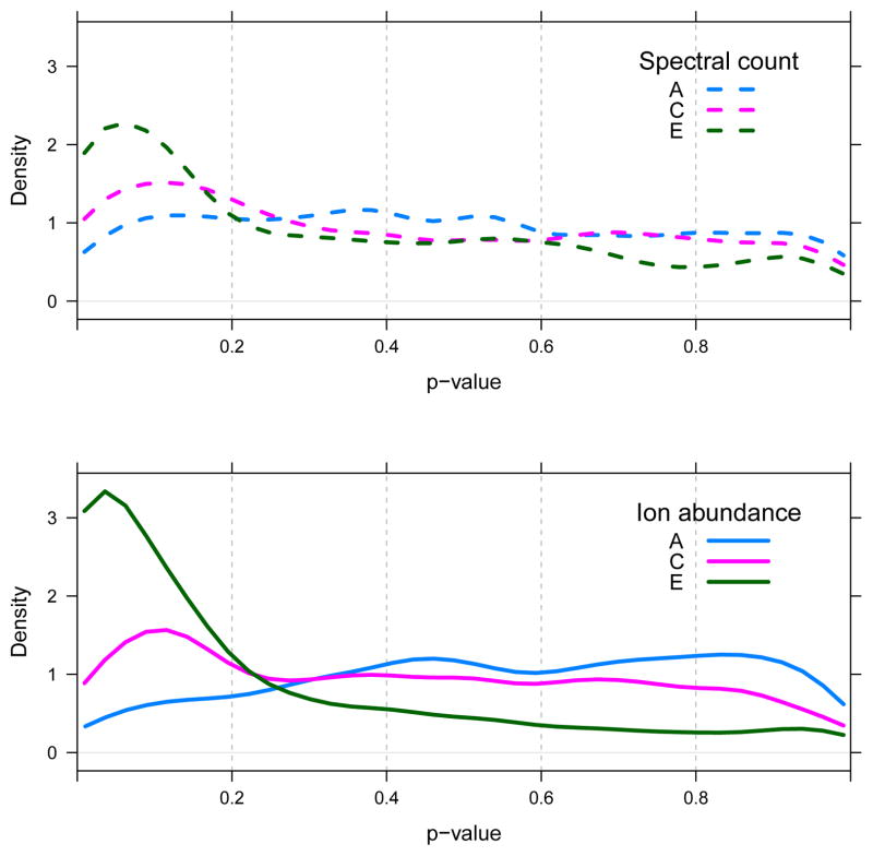
Figure 5 shows the distribution of p-values computed for the yeast proteins only of the A, C and E samples. These p-values were computed on the basis of τ_s, that is, on the basis of the spectral counts and ion abundances at the species level of rollup. Figure 5 shows that the proportion of yeast proteins determined to be significant increases as a function of increasing UPS1 protein concentration. This is the case for p-values computed using either the spectral count or ion abundance measure, though the trend is more easily seen in the ion abundance results.

Figure 5. Stratified p-values for yeast proteins.

Density estimate of the distribution of p_s for yeast proteins only of the A, C and E samples, tested against QC2, of the CPTAC data set.

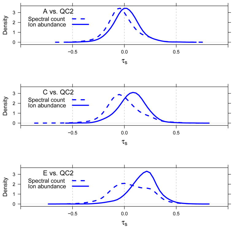
The results presented in Table 2 and Figure 5 were computed on the basis of τ_s. Figure 6 shows the distribution of τ_s for the yeast proteins only in the A, C and E samples. Note that the mass of the τ_s distributions, computed using either the spectral count or ion abundance, trend to the right as the concentration of UPS1 proteins is increased.

Figure 6. Stratified τ_s for yeast proteins.

Density estimate of the distribution of τ_s for yeast proteins only of the A, C and E samples, tested against QC2, of the CPTAC data set.

The simple structure of τ_s as an average of Wilcoxons allowed us to quickly diagnose the origin of this trend: the distribution of w for yeast species must mirror that of τ_s for yeast proteins in the A, C and E samples.

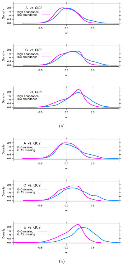
To determine the origin of the positive shift for w, we stratified w by two factors, the total ion abundance of the yeast species, and the number of missing observations of the yeast species, both in the QC2 samples. The positive trend of w does not appear to correlate with total ion abundance (Figure 7(a)). The distribution of w for few and many missing observations both trend positive as the UPS1 protein concentration increases, but the Wilcoxons for yeast species with many missing observations in QC2 appear to be influenced less (Figure 7(b)). We conclude, however, that neither factor explains the shift of w.

Figure 7. Stratified w for yeast species.

Density estimate of the distribution of the Wilcoxon statistic w for yeast species stratified by (a) the total ion abundance (low abundance is ≤ the median; high abundance is > median) and (b) the total number of missing observations (0–5 and 6–12), both as measured in the QC2 samples.

The positive shift in the distribution of w for the yeast species, and τ_s for the yeast proteins, obviously correlates with the increasing concentration of the UPS1 proteins. Consequently, we speculated that the trend is the result of a competition for ions between yeast and UPS1 species that elute in the same time window of the LC-MS experiments measuring the case samples, A, B, C, D, or E. To test this, we defined an ‘interference distance’, d_i, associated with each yeast feature i, which measures the average (over samples) minimum time separating the 2σ extent (see Equation (1)) of a yeast feature from the 2σ extent of all UPS1 features in the same sample. d_i is defined by

$$d_i=\underset{k\in \text{case}\text{samples}}{\text{mean}}\left(\underset{j\in \text{UPS}1\text{feature}}{min}{d}_{\mathit{ijk}}\right),i\in \text{yeast}\text{features},$$ (4)

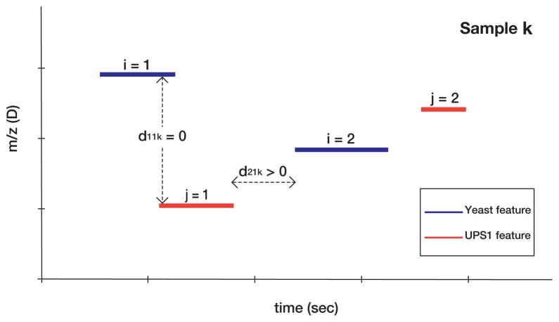
where d_ijk is (roughly) the absolute value of the time separating the i’th yeast feature from the j’th UPS1 feature in sample k. If the 2σ time extent of yeast feature i is denoted [y_L, y_R], and the 2σ time extent of UPS1 feature j is denoted [u_L, u_R], both in sample k, d_ijk is given by

$$d_{\mathit{ijk}}=\{\begin{array}{ll}{y}_L-u_R\hfill & \text{if}{y}_L>u_R,\hfill \\ u_L-y_R\hfill & \text{if}{u}_L>y_R,\hfill \\ 0\hfill & \text{otherwise}.\hfill \end{array}$$ (5)

d_ijk = 0 when the yeast and UPS1 features overlap in time and potentially compete for ions; d_ijk is taken as missing if the yeast feature i or UPS1 feature j are missing in sample k. The definition of d_ijk is illustrated in Figure 8.

Figure 8. Schematic defining the distance between LC-MS features.

d_ijk quantifies the time separation of the i’th yeast feature from the j’th UPS1 feature in sample k (see Equation (5)). The blue and red lines represent the 2σ extent of yeast and UPS1 features, respectively.

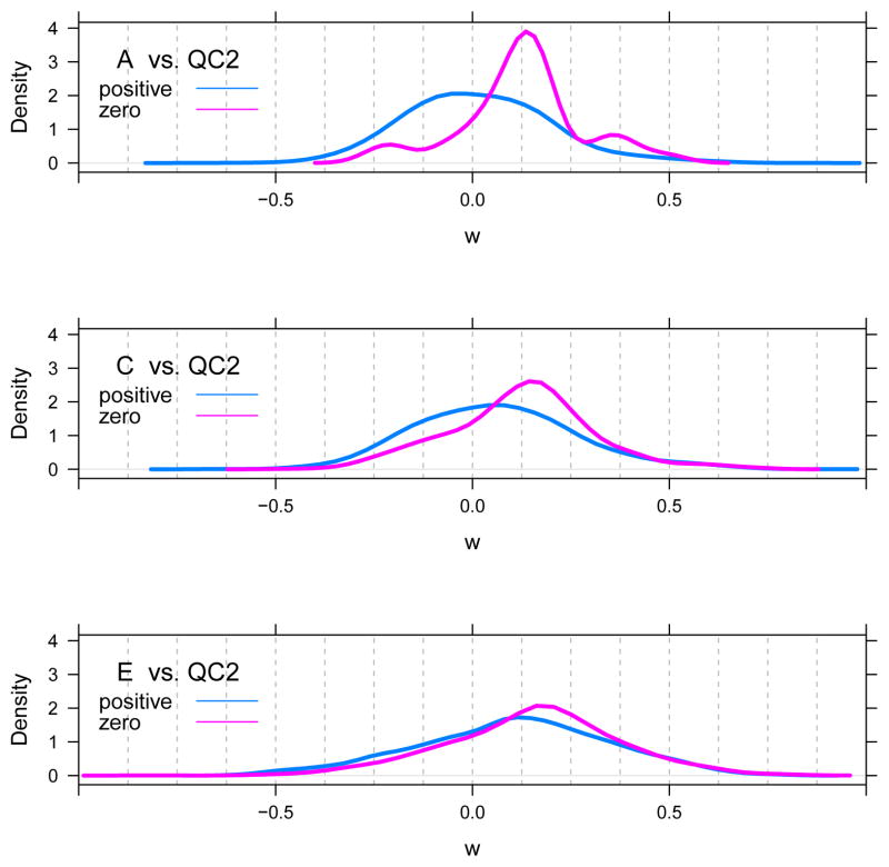
Figure 9 shows the distribution of w for the yeast species in the A, C and E samples stratified by interference distance. Table 3 shows the corresponding number of yeast species in three interference distance cohorts for samples A–E. The ‘zero’ cohort describes yeast species for which the interference distance d_i = 0; the ‘positive’ cohort includes yeast species with d_i > 0; and the ‘missing’ cohort includes yeast species for which an interference distance could not be computed.

Figure 9. Ion competition.

Density estimate of the distribution of the Wilcoxon statistic, w, for yeast species stratified by the interference distance of the yeast features from UPS1 features.

Table 3.

The number of yeast species for which the interference distance is zero, positive or missing in the A–E samples.

Sample	zero	positive	missing	total
A	39	3699	203	3941
B	189	3451	295	3935
C	682	2784	365	3831
D	1907	1673	275	3855
E	2683	690	437	3810

Note in Figure 9 that the Wilcoxons w in the zero cohort are shifted to positive values for all of the A, C and E samples. That is, the Wilcoxon is shifted for all yeast species whose feature overlaps in time with a UPS1 feature. This is consistent with our hypothesis that ion competition is responsible for the positive shift in the distribution of w for the yeast species and, consequently, the positive shift in the distribution of τ_s for the yeast proteins as well.

The Wilcoxons for yeast species in the positive cohort are centered at zero in sample A and shift slowly to more positive values as the UPS1 spike-in level increases. We hypothesized that this slow rightward shift is a result of ion competition outside the 2σ extent we assumed in assigning yeast species to the zero cohort.

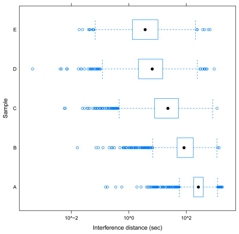
To test this, we plotted (Figure 10) the distribution of the interference distance for yeast species of the positive cohort only. Especially in sample E, the bulk of yeast features corresponding to species in the positive cohort are in close proximity to a UPS1 feature. This provides additional evidence that ion competition is responsible for the rightward shift of w seen in Figure 9. Moreover, among the yeast species in the positive cohort, their Wilcoxons and interference distances are significantly negatively correlated, based on Spearman’s rank correlation coefficient (ρ = −0.14, and the p-value for H₀: ρ = 0 is < 10⁻⁵).

Figure 10. Positive cohort interference distances.

The distribution of the interference distance for yeast species belonging to the positive cohort for samples A–E.

The yeast species in the missing cohort require comment. As is evident by examining the definition of the interference distance d_i in Equation (4), in most cases that d_i was not computed, the yeast species i will not have been observed in the case samples, one of A–E. This implies that i was observed only in the QC2 samples. Consequently, for yeast species in the missing cohort, the corresponding Wilcoxons will all be positive, i.e., these species will behave very much like the yeast species in the zero cohort with respect to their contribution to τ_s.

Note that in Table 3, excepting sample D, the number of missing yeast species increases monotonically with the increasing level of spike-in. We interpret this to mean that as additional UPS1 protein is introduced, not only is the ion abundance of yeast features reduced by competition with UPS1 features, but that an increasing number of yeast features are out-competed entirely, i.e., they are not observed, or not successfully quantified for their ion abundance.

As we saw with the BIATECH-54 data, we are able to detect characteristics of the CPTAC data set using the ion abundance only hinted at using the spectral count. In particular, we find that the ‘false positive’ detections of yeast proteins ⇓ in sample E (Table 2) are in fact not false. They reflect a true difference in sample E, apparently an artifact of ion competition between the yeast and UPS1 features in the LC-MS experiment. This competition increases as the level of spike-in of UPS1 protein increases from A to E.

4. DISCUSSION

The results of an LC-MS/MS proteomics study depend on a complex set of choices which ultimately define the ‘data’ that is analyzed. Here we presented a multi-faceted examination of two benchmarking studies, BIATECH-54 and CP-TAC, and showed how various such choices affect their analysis and interpretation. Most significantly, our analysis using the ion abundance to quantify the data exposed properties of these data sets not readily apparent from the results of a parallel analysis using the spectral count. We also showed that the level to which data is ‘rolled up’ prior to analysis may significantly affect the results and that the differences so revealed can be informative. Additionally, we reported on how the parameters used to execute the MS/MS search can affect the results. To accomplish our analysis, we introduced the straightforward statistic τ_r (Equation (2)) so as to advance our goal of contrasting transparently the influence of quantification by spectral count and ion abundance at different levels of data rollup.

Ion abundance is more sensitive than spectral count in detecting differences between the Mix 1 and Mix 2 samples of the BIATECH-54 set. Using data obtained from a search allowing only for fully-tryptic species, ion abundance performs as well or better at all levels of rollup; the greatest sensitivity is seen at the lower levels of rollup (Figure 3(a)). Using data obtained by allowing for semi-tryptic species, the ion-abundance based τ_r detects an apparent artifact of the manner in which the BIATECH-54 samples were prepared, something not detected when τ_r is computed using the spectral count. This artifact was found to arise from the existence of approximately 10–15% more strictly semi-tryptic species in Mix 1 than in Mix 2 (Figure 4(a)).

The different results found using the data searched for fully-tryptic and semi-tryptic species (Figure 3(a) and Figure 3(b)) highlights the influence of one choice made by researchers in analyzing LC-MS/MS data. The experimental design of the BIATECH-54 study implicitly assumes that proteins undergo full tryptic digestion. Constraining the MS/MS search strategy to allow for only fully-tryptic species is therefore a natural choice. Using the less constrained semi-typtic search may seem advantageous since one may identify additional species. However, the advantages of a less-constrained search come not from finding additional high-quality hits, but from a better estimation of the null, or noise, distribution that is needed to define positive hits [7]. Once the search is complete, strictly semi-tryptic hits should be filtered out [9].

In the CPTAC study, we detected evidence of increasing ion competition as the amount of UPS1 spike-in protein increases. This is weakly detectable when τ_r is computed using the spectral count but is obvious when the ion abundance is used; see Table 2 and the companion perspectives in Figures 5 and 6. The sample-dependent trends seen in these figures reveals that the abundance of yeast proteins decreases as a function of increasing UPS1 spike-in. Conceivably, this was an artifact of a quantification method that treated high/low abundance or missing features differently. However, by stratifying the Wilcoxon w on low-versus-high total ion abundance and on few-versus-many missing observations of yeast species in QC2 (Figure 7), we diagnosed that this is not the case. The existence of ion competition in the CPTAC data was confirmed by stratifying the Wilcoxon statistics for yeast species on the basis of their interference distance (see Figures 9 and 10).

Our findings for the CPTAC data raises the question as to whether the spike-in experimental design is appropriate for the construction of a benchmark case-control study. The very introduction of a spike-in appears to bias the data by ion competition. Possibly, the bias we detect is a consequence of ‘too much’ UPS1 protein having been introduced, in the E sample in particular. However, a simple calculation confirms that the average mass of yeast protein per μl of E sample exceeds that for an average UPS1 protein by approximately 20% (1.1×10⁻¹¹ grams per UPS1 protein versus 1.33 × 10⁻¹¹ grams per yeast protein, assuming ~4,500 expressed yeast proteins [29]). This suggests that one must be cautious in interpreting the results obtained from a label-free LC-MS/MS experiment, as an over-expressed collection of proteins may interfere with the ion signal measured for other classes.

Our findings differ somewhat from those of Zybailov et al. [38] who conclude that the spectral count is more reliable than ion abundance (as summarized by the RelEx method of MacCoss et al. [24]). Similarly, Old et al. [28] conclude that the spectral count is more sensitive than ion abundance (as summarized by Serac) in detecting differentially expressed proteins. On the other hand, that study also observes that the ion abundance yields more accurate estimates of protein ratios than does the spectral count and so no definitive conclusion was drawn. We note that Old et al. use one statistic for spectral count data and another statistic for ion abundance data and so it is difficult to compare their results to ours. Indeed, comparison between spectral count and ion abundance is complicated by the myriad ways in which MS and MS/MS data are quantified and summarized statistically. This is an important point: neither of the terms “spectral count” nor “ion abundance” refers to a well-defined quantification method but rather to a general approach used to define quantities that enter into the statistical analysis. Not only are there many ways to define these quantities but there are also many ways to define the statistics that ultimately summarize protein comparisons, as seen in our discussion of peptide “rollup”.

In our analyses, we have attempted to ensure that any differences observed when using spectral count versus ion abundance for quantification are not due to non-comparable aspects of the analysis. Our use of the Wilcoxon in defining τ_r for both measures of quantification at each level of rollup allows for a statistically even-handed comparison. Additionally, the MS/MS-directed approach we employed to quantify ion abundance ensures the fairness of the comparison we make between the spectral count and ion abundance as this approach quantifies the same set of CIDs in each case.

We note in passing that we investigated a variant of τ_r computed using the t-statistic. We found the performance of this variant is less attractive than that based on the Wilcoxon. This is a consequence of the small sample size of the case studies and the parametric assumptions underlying the use of the t-statistic.

Finally, there are a variety of reasons to favor ion abundance for quantification. The statistical models for protein rollup by Clough et al. [3], for example, are implicitly based on ion abundances. Also, as noted by Podwojski et al. [30] and Lundgren et al. [23], spectral counts may be dominated by a few proteins having a large number of counts, and the spectral count breaks down as a statistical quantity when very few counts are observed. Although the estimated ion abundance of an identified species is subject to low signal and the stochastic nature of the CID sampling, it has the potential to more robustly quantify seldom-seen species.

References

- 1.Bondarenko P, Chelius D, Shaler T. Identification and relative quantitation of protein mixtures by enzymatic digestion followed by capillary reversed-phase liquid chromatography-tandem mass spectrometry. Analytical chemistry. 2002;74(18):4741–4749. doi: 10.1021/ac0256991. [DOI] [PubMed] [Google Scholar]
- 2.Choi H, Fermin D, Nesvizhskii AI. Significance analysis of spectral count data in label-free shotgun proteomics. Mol Cell Proteomics. 2008;7:2373–2385. doi: 10.1074/mcp.M800203-MCP200. [DOI] [PMC free article] [PubMed] [Google Scholar]
- 3.Clough T, Key M, Ott I, Ragg S, Schadow G, Vitek O. Protein quantification in label-free LC-MS experiments. Journal of Proteome Research. 2009;8:5275–5284. doi: 10.1021/pr900610q. [DOI] [PubMed] [Google Scholar]
- 4.Cox J, Mann M. MaxQuant enables high peptide identification rates, individualized p.p.b-range mass accuracies and proteome-wide protein quantification. Nature Biotechnology. 2008;26:1367–1372. doi: 10.1038/nbt.1511. [DOI] [PubMed] [Google Scholar]
- 5.Craig R, Beavis RC. TANDEM: matching proteins with tandem mass spectra. Bioinformatics. 2004;20:1466–1467. doi: 10.1093/bioinformatics/bth092. [DOI] [PubMed] [Google Scholar]
- 6.Deutsch EW, Lam H, Aebersold R. Data analysis and bioinformatics tools for tandem mass spectrometry in proteomics. Physiological genomics. 2008;33(1):18–25. doi: 10.1152/physiolgenomics.00298.2007. [DOI] [PubMed] [Google Scholar]
- 7.Ding Y, Choi H, Nesvizhskii AI. Adaptive discriminant function analysis and reranking of MS/MS database search results for improved peptide identification in shotgun proteomics. Journal of Proteome Research. 2008;7(11):4878–4889. doi: 10.1021/pr800484x. [DOI] [PMC free article] [PubMed] [Google Scholar]
- 8.Domon B, Aebersold R. Options and considerations when selecting a quantitative proteomics strategy. Nature biotechnology. 2010;28(7):710–721. doi: 10.1038/nbt.1661. [DOI] [PubMed] [Google Scholar]
- 9.Elias JE, Gygi SP. Target-decoy search strategy for increased confidence in large-scale protein identifications by mass spectrometry. Nature methods. 2007;4(3):207–214. doi: 10.1038/nmeth1019. [DOI] [PubMed] [Google Scholar]
- 10.Eng JK, McCormack AL, Yates JR., III An approach to correlate tandem mass spectral data of peptides with amino acid sequences in a protein database. J Am Soc Mass Spectrom. 1994;5:976–989. doi: 10.1016/1044-0305(94)80016-2. [DOI] [PubMed] [Google Scholar]
- 11.Fu X, Gharib SA, Green PS, Aitken ML, Frazer DA, Park DR, Vaisar T, Heinecke JW. Spectral Index for Assessment of Differential Protein Expression in Shotgun Proteomics. Journal of Proteome Research. 2008;7(3):845–854. doi: 10.1021/pr070271+. [DOI] [PubMed] [Google Scholar]
- 12.Griffin NM, Yu J, Long F, Oh P, Shore S, Li Y, Koziol JA, Schnitzer JE. Label-free, normalized quantification of complex mass spectrometry data for proteomic analysis. Nature Biotechnology. 2009;28:83–89. doi: 10.1038/nbt.1592. [DOI] [PMC free article] [PubMed] [Google Scholar]
- 13.Ishihama Y, Oda Y, Tabata T, Sato T, Nagasu T, Rappsilber J, Mann M. Exponentially modified protein abundance index (emPAI) for estimation of absolute protein amount in proteomics by the number of sequenced peptides per protein. Molecular & Cellular Proteomics. 2005;4(9):1265. doi: 10.1074/mcp.M500061-MCP200. [DOI] [PubMed] [Google Scholar]
- 14.Jaffe JD, Mani DR, Leptos K, Church GM, Gillette MA, Carr SA. PEPPeR, a platform for experimental proteomic pattern recognition. Mol Cell Proteomics. 2006;5:1927–1941. doi: 10.1074/mcp.M600222-MCP200. [DOI] [PMC free article] [PubMed] [Google Scholar]
- 15.Käll L, Storey JD, MacCoss MJ, Noble WS. Assigning significance to peptides identified by tandem mass spectrometry using decoy databases. Journal of Proteome Research. 2008;7:29–34. doi: 10.1021/pr700600n. [DOI] [PubMed] [Google Scholar]
- 16.Karpievitch Y, Stanley J, Taverner T, Huang J, Adkins JN, Ansong C, Heffron F, Metz TO, Qian WJ, Yoon H, Smith RD, Dabney AR. A statistical framework for protein quantitation in bottom-up MS-based proteomics. Bioinformatics. 2009;25(16):2028–2034. doi: 10.1093/bioinformatics/btp362. [DOI] [PMC free article] [PubMed] [Google Scholar]
- 17.Keller A, Nesvizhskii AI, Kolker E, Aebersold R. Empirical statistical model to estimate the accuracy of peptide identifications made by MS/MS and database search. Anal Chem. 2002;74:5383–5392. doi: 10.1021/ac025747h. [DOI] [PubMed] [Google Scholar]
- 18.Kolker E, Hogan JM, Higdon R, Kolker N, Landorf E, Yakunin AF, Collart FR, van Belle G. Development of BIATECH-54 standard mixtures for assessment of protein identification and relative expression. Proteomics. 2007;7:3693–3698. doi: 10.1002/pmic.200700088. [DOI] [PubMed] [Google Scholar]
- 19.Leptos KC, Sarracino DA, Jaffe JD, Krastins B, Church GM. MapQuant: open-source software for large-scale protein quantification. Proteomics. 2006;6:1770–1782. doi: 10.1002/pmic.200500201. [DOI] [PubMed] [Google Scholar]
- 20.Li XJ, Yi EC, Kemp CJ, Zhang H, Aebersold R. A software suite for the generation and comparison of peptide arrays from sets of data collected by liquid chromatography-mass spectrometry. Mol Cell Proteomics. 2005;4:1328–1340. doi: 10.1074/mcp.M500141-MCP200. [DOI] [PubMed] [Google Scholar]
- 21.Liu H, Sadygov R, Yates J., III A model for random sampling and estimation of relative protein abundance in shotgun proteomics. Analytical chemistry. 2004;76(14):4193–4201. doi: 10.1021/ac0498563. [DOI] [PubMed] [Google Scholar]
- 22.Lu P, Vogel C, Wang R, Yao X, Marcotte E. Absolute protein expression profiling estimates the relative contributions of transcriptional and translational regulation. Nature biotechnology. 2006;25(1):117–124. doi: 10.1038/nbt1270. [DOI] [PubMed] [Google Scholar]
- 23.Lundgren D, Hwang S, Wu L, Han D. Role of spectral counting in quantitative proteomics. Expert Review of Proteomics. 2010;7(1):39–53. doi: 10.1586/epr.09.69. [DOI] [PubMed] [Google Scholar]
- 24.MacCoss MJ, Wu CC, Liu H, Sadygov R, Yates JR. A Correlation Algorithm for the Automated Quantitative Analysis of Shotgun Proteomics Data. Analytical Chemistry. 2003;75(24):6912–6921. doi: 10.1021/ac034790h. [DOI] [PubMed] [Google Scholar]
- 25.Milac TI, Wang P, Randolph TW. Sahale: A software suite to quantify, analyze and visualize data from LC-MS/MS experiments. 2012 In preparation. See http://sahale.fhcrc.org.
- 26.Mueller LN, Rinner O, Schmidt A, Letarte S, Bodenmiller B, Brusniak MY, Vitek O, Aebersold R, Müller M. SuperHirn - a novel tool for high resolution LC-MS-based peptide/protein profiling. Proteomics. 2007;7:3470–3480. doi: 10.1002/pmic.200700057. [DOI] [PubMed] [Google Scholar]
- 27.Neilson K, Ali N, Muralidharan S, Mirzaei M, Mariani M, Assadourian G, Lee A, van Sluyter S, Haynes P. Less label, more free: Approaches in label-free quantitative mass spectrometry. Proteomics. 2011;11:535–553. doi: 10.1002/pmic.201000553. [DOI] [PubMed] [Google Scholar]
- 28.Old WM, Meyer-Arendt K, Aveline-Wolf L, Pierce KG, Mendoza A, Sevinsky JR, Resing KA, Ahn NG. Comparison of label-free methods for quantifying human proteins by shotgun proteomics. Molecular and Cellular Proteomics. 2005;4:1487–1502. doi: 10.1074/mcp.M500084-MCP200. [DOI] [PubMed] [Google Scholar]
- 29.Paulovich AG, Billheimer D, Ham AL, Vega-Montoto L, Rudnick PA, Tabb DL, Wang P, Blackman RK, Bunk DM, Cardasis HL, Clauser KR, Kinsinger CR, Schilling B, Tegeler TJ, Variyath AM, Wang M, Whiteaker JR, Zimmerman LJ, Fenyo D, Carr SA, Fisher SJ, Gibson BW, Mesri M, Neubert TA, Regnier F, Rodriguez H, Spiegelman C, Stein SE, Tempst P, Liebler DC. Interlaboratory study characterizing a yeast performance standard for benchmarking LC-MS platform performance. Molecular & Cellular Proteomics. 2010;9:242–254. doi: 10.1074/mcp.M900222-MCP200. [DOI] [PMC free article] [PubMed] [Google Scholar]
- 30.Podwojski K, Eisenacher M, Kohl M, Turewicz M, Meyer HE, Rahnenfuhrer J, Stephan C. Peek a peak: a glance at statistics for quantitative label-free proteomics. Expert Review of Proteomics. 2010;7(2):249–261. doi: 10.1586/epr.09.107. [DOI] [PubMed] [Google Scholar]
- 31.Sigma-Aldrich. UPS1 Universal Proteomics Standard Set. 2011 http://www.sigmaaldrich.com.
- 32.Sing T, Sander O, Beerenwinkel N, Lengauer T. ROCR: visualizing classifier performance in R. Bioinformatics. 2005;21(20):3940–3941. doi: 10.1093/bioinformatics/bti623. [DOI] [PubMed] [Google Scholar]
- 33.Storey JD, Tibshirani R. Statistical significance for genome-wide studies. Proceedings of the National Academy of Sciences. 2003;100:9440–9445. doi: 10.1073/pnas.1530509100. [DOI] [PMC free article] [PubMed] [Google Scholar]
- 34.Tabb DL, Fernando CG, Chambers MC. Myri-Match: highly accurate tandem mass spectral peptide identification by multivariate hypergeometric analysis. J Proteome Res. 2007;6:654–661. doi: 10.1021/pr0604054. [DOI] [PMC free article] [PubMed] [Google Scholar]
- 35.Wang P, Liu Y. R package version 0.1-1. 2008. SASPECT: Significant AnalysiS of PEptide CounTs. [Google Scholar]
- 36.Whiteaker JR, Zhang H, Zhao L, Wang P, Kelly-Spratt KS, Ivey RG, Piening BD, Feng LC, Kasarda E, Gurley KE, Eng JK, Chodosh LA, Kemp CJ, McIntosh MW, Paulovich AG. Integrated pipeline for mass spectrometry-based discovery and confirmation of biomarkers demonstrated in a mouse model of breast cancer. J Proteome Res. 2007;6:3962–3975. doi: 10.1021/pr070202v. [DOI] [PubMed] [Google Scholar]
- 37.Zhang B, VerBerkmoes N, Langston M, Uberbacher E, Hettich R, Samatova N. Detecting differential and correlated protein expression in label-free shotgun proteomics. Journal of Proteome Research. 2006;5(11):2909–2918. doi: 10.1021/pr0600273. [DOI] [PubMed] [Google Scholar]
- 38.Zybailov B, Coleman M, Florens L, Washburn M. Correlation of relative abundance ratios derived from peptide ion chromatograms and spectrum counting for quantitative proteomic analysis using stable isotope labeling. Analytical Chemistry. 2005;77(19):6218–6224. doi: 10.1021/ac050846r. [DOI] [PubMed] [Google Scholar]