

Abstract
Clustering analysis is an important tool in studying gene expression data. The Bayesian hierarchical clustering (BHC) algorithm can automatically infer the number of clusters and uses Bayesian model selection to improve clustering quality. In this paper, we present an extension of the BHC algorithm. Our Gaussian BHC (GBHC) algorithm represents data as a mixture of Gaussian distributions. It uses normal-gamma distribution as a conjugate prior on the mean and precision of each of the Gaussian components. We tested GBHC over 11 cancer and 3 synthetic datasets. The results on cancer datasets show that in sample clustering, GBHC on average produces a clustering partition that is more concordant with the ground truth than those obtained from other commonly used algorithms. Furthermore, GBHC frequently infers the number of clusters that is often close to the ground truth. In gene clustering, GBHC also produces a clustering partition that is more biologically plausible than several other state-of-the-art methods. This suggests GBHC as an alternative tool for studying gene expression data.
The implementation of GBHC is available at https://sites.google.com/site/gaussianbhc/
Introduction
Clustering analysis is an important tool in studying genomic data such as gene expression profiles and can be used to infer biological function and regulation of genes. Eisen et al. [1] found that in yeast S. cerevisiae, genes that are clustered together often share similar biological function or are co-regulated, leading to the recognition that genes in the same cluster can be functionally related or regulated by a common set of transcription factors. It has been shown in the literature that biological function of a cluster can be inferred from ontology annotation of its genes [2], and biological function of an uncharacterized gene can also be inferred from the knowledge of genes in its cluster [3], [4]. Moreover, in modern medical research, clustering analysis has been used to identify disease subtypes based on genetic variation [5], [6], and to identify a gene expression signature that can be used as a prognostic marker for known disease subtypes [7]–[9]. This aids stratification of patients for personalized medicine.
Numerous commonly used clustering algorithms have a significant limitation in that they rely on ad hoc methods to identify the number of clusters within the data. In hierarchical clustering algorithms [10]–[12], for example, identifying the number of clusters mainly depends on visual identification, whereas the number of clusters is required as an input to other algorithms such as  -means [13] and self-organizing map [14]. Furthermore, many clustering algorithms require the choice of a distance metric to indicate the strength of similarity/dissimilarity between data points or clusters. However, there is little systematic guidance about how to choose a metric for data such as gene expression measurements that reflects reasonably well the relationship between data. Often, it is difficult to define the relationship, especially in high-dimensional space. Two common choices of metrics in gene clustering analysis literature are Euclidean distance and Pearson correlation coefficient [15]. However, Euclidean distance is sensitive to scaling and differences in average. Pearson correlation coefficient can only capture linear relationship between data, and it is not robust to outliers and non-Gaussian distribution [16]. Model-based clustering algorithms can address both of these problems. In model-based algorithms, data are represented by a mixture model [17], [18] of parameterized distributions, in which each component represents a different cluster. The problems of how to identify the number of clusters and the distance metric can therefore be cast as a model selection problem - how to choose a statistical model that best describes the data.
Bayesian hierarchical clustering (BHC) [19], [20] is a model-based clustering algorithm based on the Dirichlet process mixture model (DPM) [18], [21], [22]. It has strong advantages over other model-based approaches. First, it produces a hierarchical clustering structure which is more informative than a flat one. Second, it uses Bayesian model selection to determine the hierarchical structure, rather than an ad hoc distance metric, thereby increasing the quality of resulting clusters. Multinomial BHC (MBHC) [23] represents the data in each mixture component as a product of multinomial likelihoods, subject to a Dirichlet prior, and has been shown to produce higher dendrogram purity and more biologically meaningful clusters than other commonly used algorithms for the Arabidopsis thaliana microarray dataset [23]. However, by using multinomial likelihoods, the algorithm requires a categorical approximation of a continuous variable. This may not, therefore, fully capture the underlying structure of continuous gene expression data. Gaussian likelihoods are an obvious alternative here, as they do not require data approximation and have been used for describing gene expression data in many clustering analyses. Previous work on expression datasets of ovary and yeast cell cycle show that model-based clustering algorithms that use finite Gaussian mixture model produce comparable quality clusters to a leading heuristic clustering algorithm, even if the data do not totally satisfy Gaussian mixture assumption [24]. In a comparative study of clustering algorithms for cancer gene expression data, given the actual number of clusters, finite Gaussian model approach is the leader in assigning data to the correct cluster [25]. Rasmussen et al. [26] propose a model-based clustering algorithm with infinite Gaussian mixture model to study Rosetta compendium of expression profiles of S. cerevisiaie, and find that clustering results not only confirm previously published clustering analyses but also reveal finer clustering level that are novel and biologically consistent.
In this paper, we propose an extension of the BHC algorithm for gene expression data which we term as the Gaussian BHC (GBHC). GBHC offers several advantages over other clustering algorithms: first, it assumes an infinite Gaussian mixture model for gene expression data, which has been shown to be biologically plausible in literature [24]–[26]; second, it employs the mixture model in a Bayesian framework to perform a model-based hierarchical clustering of gene expression data revealing hierarchical structure present in the data; third, it infers the number of clusters automatically from the data; and fourth, it uses the Gaussian mixture assumption to describe the data and uses a normal-gamma distribution as a conjugate prior on unknown means and precisions of the Gaussian likelihoods. We introduce two variants of GBHC: one with hyperparameter optimization over the whole tree (GBHC-TREE), and another with hyperparameter optimization at every merger (GBHC-NODE). Further, we derive a tractable formulation for speeding up the hyperparameter optimization in case of GBHC-NODE, resulting in a speedup factor of up to 11 over GBHC-TREE. We compare these two algorithms with a range of other clustering methods, performing a study over 3 synthetic datasets and 11 cancer gene expression datasets. The results show that although the data are not very well-represented by a mixture of Gaussian distributions, both variants still improve the clustering quality if the data are normalized and do not have strong correlation between variables. On average, both flavors of our GBHC algorithm produce clustering results which compare favorably to the existing approaches.
Materials and Methods
Notations

|
unknown parameters of a probabilistic model component in a mixture model |

|
hyperparameters of a prior on 
|

|
indices |

|
a data value of the  variable from the variable from the  observation observation |

|
total number of data variables |

|
a data point 
|

|
the  cluster of data points, respectively cluster of data points, respectively |

|
a merger that makes  , respectively , respectively |

|
number of data points in 
|

|
concentration parameter of the Dirichlet process mixture model |

|
merger probability |

|
hyperparameters of the marginal likelihood for a Gaussian distribution with a normal-gamma prior |

|
probability |

|
gamma function |

|
digamma function, defined by 
|

|
probability density function of a Gaussian distribution |

|
probability density function of a normal-gamma distribution |

|
probability density function of a gamma distribution |
Bayesian Hierarchical Clustering Algorithm
BHC [19] assumes that data are generated from a mixture model, in which each cluster within the data corresponds to a different distribution component of the model. Suppose that data points  in a cluster
  are independently and identically generated from a probabilistic model
  with unknown parameters
  , and
, and  are governed by a prior
  with hyperparameters
  . Thus, the marginal likelihood of
  can be expressed by
 |
(1) |
The algorithm initially places each data point into its own trivial cluster and iteratively merges the two most similar clusters, until all the data points are put into a single cluster. This merger process can be represented by a dendrogram (Figure 1A).
Figure 1. Bayesian hierarchical clustering.
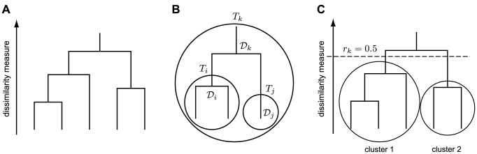
A) A dendrogram represents the merger process of BHC. Each vertical line represents a cluster. A horizontal line connecting between any two vertical lines represents the merger of clusters, where its height is related to the dissimilarity measure between the merged clusters. B) A schematic shows datasets  and
and  merged into
  , where
  , and
, and  are the associated mergers that make
  , and
, and  , respectively. C) BHC prunes the dendrogram at
  , resulting in the final partition.
The notion of similarity between clusters is related to the probability that they should be merged. This is defined based on Bayesian hypothesis testing as follows. To merge clusters  and
and  into
into  (Figure 1B), BHC considers the null hypothesis
  :
:  and
and  belong to
  and the alternative hypothesis
  :
:  consists of two or more clusters. The probability that
  and
and  should be merged is calculated via the Bayes' rule:
| (2) |
where a marginal likelihood  is defined recursively by
| (3) |
 is a marginal likelihood of
  given in Equation (1), and
  is a prior that
  and
and  should be merged and is defined recursively by
| (4) |
| (5) |
where we set  and
and  for every initial cluster
  . We note that the definition of
  defined here makes Equation (3) an approximation of a marginal likelihood of DPM. Moreover, the value of concentration parameter
  is connected to the expected number of clusters that BHC infers. An increase in
  implies an increase in the expected number of clusters.
At  ,
,  and
and  are more likely to belong to the same cluster than at
  . Consequently, we obtain the final number of clusters and partition when all the remaining pairs of merger have
  (Figure 1C).
The Marginal Likelihood for Gaussian Distribution with Unknown Mean and Precision
Consider a dataset in which each observation  consists of
  variables, i.e.
 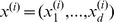 . We assume that
A 1 the dataset is normalized, i.e. it has mean zero and a unit variance;
A 2 for each observation  , its variables
  are independent and generated from different Gaussian distributions;
A 3 the realizations of each variable  ,
,  in cluster
  are independent and identically distributed and drawn from Gaussian distribution with unknown mean
  and precision
  , and the prior on
  is a normal-gamma distribution with hyperparameter
  .
.
The probability density function of a Gaussian distribution is defined as
| (6) |
and the probability density function of a normal-gamma distribution is defined as
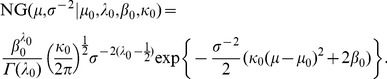 |
(7) |
From the above assumptions, the marginal likelihood of  can be expressed as
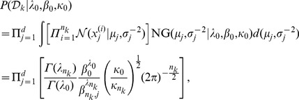 |
(8) |
where
| (9) |
and
| (10) |
| (11) |
| (12) |
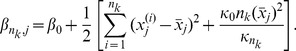 |
(13) |
In deriving (8), the hyperparameter  which indicates the mean of parameter
  is set to
  to reflect Assumption A1. Equation (8) is all that is required for
  in GBHC.
Hyperparameter Optimization
GBHC infers the values of hyperparameters  by using the information from
  which tells us how well the clustering hierarchy fits the data. This inference can be done via two optimization schemes as follows.
- Optimization globally over the whole tree (TREE). GBHC-TREE finds only one set of optimal hyperparameters
 that fits the whole data, and is given by
where
(14)  is the marginal likelihood (3) of the final merger in BHC. To learn the optimal hyperparameters in this case is costly since the gradients of
  with respect to hyperparameters are analytically intractable, unless the structure of the clustering hierarchy is fixed. (See [19] for more details on optimization of
  in the case that the clustering hierarchy is fixed.)
 - Optimization at every merger (NODE). GBHC-NODE finds optimal hyperparameters

 for each merger
  in BHC by performing
where
(15)
and we assume that
(16) 
(17) 
(18)
The probability density function of a Gamma distribution is defined by
(19)
Thus the log-likelihood function in (16) can be written as,
(20)
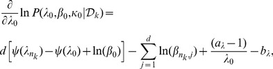
and its gradients with respect to hyperparameters are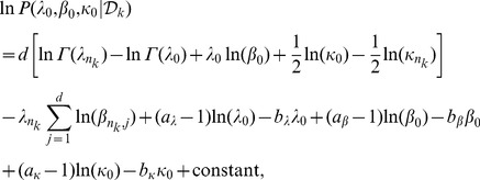
(21) 
(22) 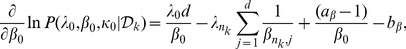
(23)
See Section S1 in Material S1 for derivations of Equations (22)–(24). We use weakly informative priors over hyperparameters in Equations (17)–(19), assuming that the data are normalized,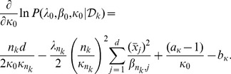
(24)
We note that Equation (15) is related to the optimization of
(25)  , in which approximation
 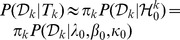 and the maximization of its posterior distribution is considered. We can see that GBHC-NODE finds the optimal structure of the clustering hierarchy in a single run by searching for the best merger at each level while the hierarchy is constructed. So, it is more time-efficient than GBHC-TREE.
The possible limitation of both optimization schemes is that the optimization objective functions (14),(15) can be non-convex. This will result in GBHC-TREE and GBHC-NODE only finding hyperparameters that are locally optimal. Nevertheless, in our experiments with clustering synthetic data and gene expression data, both schemes have produced promising results.
Other Clustering Algorithms
We compare GBHC-TREE and GBHC-NODE to other clustering algorithms in Table 1. The algorithms and their similarity/dissimilarity measure will be referred to by the abbreviations given in the table. For instance, APE stands for affinity propagation using negative Euclidean distance. Furthermore, we employ L-methods [27] to infer the number of clusters in AC,AE,CC,CE,KC, and KE, which are the algorithms that require pre-specified number of clusters.
Table 1. Clustering algorithm.
| Algorithm | Similarity/Dissimilarity Metric | Ability to Infer # Clusters | Reference |
| AP: affinity propagation | C: negative one minus Pearson's correlation coefficient; E: negative Euclidean distance | yes | [32] |
| MBHC: multinomial BHC | - | yes | [19], [23] |
| A: average-linkage hierarchical clustering | C: one minus Pearson's correlation coefficient; E: Euclidean distance | no | [10] |
| C: complete-linkage hierarchical clustering | C: one minus Pearson's correlation coefficient; E: Euclidean distance | no | [11], [12], [33] |
| K: k-means | C: one minus Pearson's correlation coefficient; E: square Euclidean distance | no | [13] |
In this work, we implement GBHC-TREE, GBHC-NODE and MBHC in MATLAB. We use AP which is publicly available at the authors' webpage (http://www.psi.toronto.edu/index.php?q=affinity\%20propagation). All the remaining algorithms could be found as MATLAB's built-in functions.
The Datasets
Synthetic Datasets
GBHC-TREE and GBHC-NODE should perform very well if the Assumptions A1–A3 are satisfied. However, real expression data are expected to be not fully satisfied Gaussian mixture assumption, and the correlation between data variables is possible. It is very important to evaluate the performance of GBHC-TREE and GBHC-NODE in comparison to the other clustering algorithms when some of the assumptions are violated. Here, we use synthetic datasets to study GBHC-TREE and GBHC-NODE in three different scenarios as follows (see Section S2 in Material S1 for more details on how the data are generated).
Synthetic Dataset1: Mixture of Gaussian Distributions and Independent Data Variables
1000 observations of 10-dimensional random vector are drawn from a mixture of 7 multivariate Gaussian distributions, where each multivariate Gaussian distribution has diagonal covariance matrix. Then the data are normalized.
Synthetic Dataset2: Mixture of Gaussian Distributions and Correlated Data Variables
Similar to the first scenario, 1000 observations of 10-dimensional random vector are drawn from a mixture of 7 multivariate Gaussian distributions, but the covariance matrix of each multivariate Gaussian distribution has non-diagonal entries which are non-zero. Then the data are normalized.
Synthetic Dataset3: Mixture of Several Distributions
We generate 1000 observations of 10-dimensional random vector from a mixture of 7 different multivariate distributions. For the first 6 multivariate components of a mixture, namely Gaussian, gamma, uniform, student's t, Weibull, and chi-squared distributions, random variables in different dimensions are independent. For the last multivariate component of a mixture which is a Gaussian distribution, there is correlation between random variables in different dimensions. This dataset is normalized prior to the use.
Gene Expression Datasets
The performance of all the aforementioned clustering algorithms is assessed through 11 cancer datasets, as described in Table 2. Blood1, Blood2, Bone Marrow, Brain1, Brain2, Colon, Multi-tissue1, Multi-tissue2, Prostate1 are downloaded from http://algorithmics.molgen.mpg.de/Static/Supplements/CompCancer/datasets.htm. These datasets are already filtered according to the protocol described in [25]. We transform every dataset by  and normalize it before using.
Table 2. Dataset detail.
| Dataset Name | # Total Samples | # Classes | Classes | # Total Probes | # Remaining Probes |
| Blood1 [34] | 72 | 2 | 24 ALL, 48 MLL | 12,582 | 1,081 |
| Blood2 [35] | 77 | 2 | 58 DLBCL, 19 FL | 7,129 | 798 |
| Bone Marrow [36] | 72 | 2 | 47 ALL, 25 AML | 7,129 | 1,868 |
| Brain1 [37] | 28 | 2 | 14 CG, 14 NG | 12,625 | 1,070 |
| Brain2 [38] | 42 | 5 | 10 MD, 10 Mglio, 10 Rhab, 4 Ncer, 8 PNET | 7,129 | 1,379 |
| Colon [39] | 37 | 2 | 8 serrated CRC, 29 conventional CRC | 22,883 | 2,202 |
| Lung | 16 | 3 | 7 NL, 5 LCNEC, 4 SCLC | 42,545 | 2,995 |
| Multi-tissue1 [40] | 190 | 14 | 11 BR, 10 PR, 11 LU, 11 CRC, 22 LY, 10 ML, 11 BL, 10 UT, 30 LE, 11 RE, 11 PA, 11 OV, 11 ME, 20 CNS | 16,063 | 1,363 |
| Multi-tissue2 [41] | 174 | 10 | 26 PR, 8 BL, 26 BR, 23 CRC, 12 GA, 11 KI, 7 LI, 27 OV, 6 PA, 28 LU | 12,533 | 1,571 |
| Prostate1 [42] | 102 | 2 | 50 NP, 52 PR | 12,600 | 339 |
| Prostate2 [43] | 19 | 3 | 6 benign, 7 primary, 6 metastatic | 54,675 | 1,348 |
ALL: acute lymphoblastic leukemia; AML: acute myelogenous leukemia; BL: bladder/ureter cancer; BR: breast cancer; CG: classic glioblastoma; CNS: central nervous system; CRC: colorectal cancer; DLBCL: diffuse large B-cell lymphoma; FL: follicular lymphoma; GA: esophageal cancer; KI: kidney cancer; LCNEC: large cell neuroendocrine carcinoma; LE: leukemia; LI: liver cancer; LU: lung cancer; LY: lymphoma; MD: medulloblastoma; ME: pleural mesothelioma; Mglio: malignant glioma; ML: melanoma; MLL: lymphoblastic leukemia with myeloid/lymphoid or mixed-lineage leukemia (MLL) translocations; Ncer: normal cerebella; NG: nonclassic glioblastoma; NL: normal lung tissue; NP: normal prostate tissue; OV: ovarian cancer; PA: pancreatic cancer; PNET: primitive neuroectodermal tumour; PR: prostate cancer; RE: renal cell carcinoma; Rhab: atypical teratoid/rhabdoid tumour; SCLC: small cell lung carcinoma; UT: uterine cancer;
Prostate2 is downloaded from Gene Expression Omnibus (http://www.ncbi.nlm.nih.gov/geo/) (GDS1439). The dataset is transformed by  and then filtered by the Wilcoxon rank-sum test at significance level 0.001. The test is carried out between a group of benign and a group of primary and metastatic. The dataset is normalized before using.
Lung is available at Gene Expression Omnibus (GSE44447). The microarray experiment of this data was conducted on Agilent SurePrint G3 Human Gene Expression 8×60 K microarrays (AGilent Technologies, Wokingham, UK), using lung tissues that were ethically approved under the Multicentre Research Ethics Committee (MREC) approval. The experiment was designed to compare the gene expression profiles of two types of closely related high grade neuroendocrine carcinomas, small cacinoma and large cell neuroendocrine carcinoma, which are difficult to classify correctly even for pulmonary pathologists. The raw expression data was processed using R Bioconductor package limma (http://www.bioconductor.org/packages/2.10/bioc/html/limma.html), loess and quantiled normalized and corrected for batch effect using ComBat (http://www.bu.edu/jlab/wp-assets/ComBat/Abstract.html). We filter this dataset using Wilcoxon rank-sum test for testing the difference between normal and cancer groups at significance level 0.001, and normalize it prior to clustering.
Clustering Performance Indices
We use two metrics to evaluate the clustering performance: (i) adjusted Rand index (ARI) [28] and, (ii) biological homogeneity index (BHI) [29]. In the clustering of synthetic data, since the true partition of data classes is known, ARI is used as a measure of agreement between clustering partition and the true partition. ARI scores a pair of partitions between 0 and 1, and a higher ARI score indicates higher agreement. We also use ARI in sample clustering experiment of gene expression data.
In gene clustering of gene expression data, we are interested in how biologically meaningful the clustering results are. BHI is used to measure the biological plausibility of gene clustering results generated by an algorithm. It scores a partition between 0 and 1, where a higher score will be assigned to the more biological homogeneous partition based on a reference set of functional classes. In this case, we use Gene Ontology (GO) annotation in Bioconductor package (Section S3, Table S1 in Material S1), while the BHI is calculated using the R package clValid [30].
Results and Discussion
Synthetic Datasets
ARI scores of clustering algorithms are shown in Table 3, and the numbers of clusters inferred by the algorithms are given in Section S5, Table S2 in Material S1. Details of the experimental setting can also be found in Section S4 in Material S1. For visual inspection of clustering results, we employ a dimension reduction approach called t-Distributed Stochastic Neighbor Embedding (t-SNE) [31] algorithm to reduce the dimension of the original synthetic data into 2-dimensional Euclidean space. t-SNE maps data by preserving the local structure; thus data which are in the same cluster will be placed close by each other in the lower-dimensional space. The visualizations of clustering results are shown in Figures 2, 3, 4.
Table 3. Adjusted Rand Index from Synthetic Data Clustering Experiment.
| Dataset | APC | APE | GBHC-TREE | GBHC-NODE | MBHC | AC | AE | CC | CE | KC | KE |
| Synthetic Dataset1 | 0.317 | 0.230 | 1.000 | 1.000 | 0.648 | 0.938 | 0.996 | 0.932 | 0.954 | 0.547 | 0.851 |
| Synthetic Dataset2 | 0.106 | 0.095 | 0.467 | 0.270 | 0.143 | 0.324 | −0.000 | 0.132 | 0.088 | 0.312 | 0.413 |
| Synthetic Dataset3 | 0.295 | n/a | 0.897 | 0.921 | 0.643 | 0.479 | 0.002 | 0.710 | 0.506 | 0.495 | 0.750 |
| mean | 0.239 | 0.163 | 0.788 | 0.730 | 0.478 | 0.581 | 0.333 | 0.592 | 0.516 | 0.451 | 0.671 |
n/a: not applicable since the algorithm does not converge. Bold number(s) in each dataset highlight(s) the maximum ARI value. Bold underlined numbers highlight the first three highest average ARIs.
Figure 2. Clustering Results of Synthetic Dataset1.

Clusters are represented by different colors or types of marker. A) 7 actual clusters. B) Clustering result produced by GBHC-TREE has 7 clusters. C) Clustering result produced by GBHC-NODE has 7 clusters. D) Clustering result produced by AE has 7 clusters.
Figure 3. Clustering Results of Synthetic Dataset2.

Clusters are represented by different colors or types of marker. A) 7 actual clusters. B) clustering result produced by GBHC-TREE has 14 clusters. C) clustering result produced by GBHC-NODE has 37 clusters. D) clustering result produced by KE has 4 clusters.
Figure 4. Clustering Results of Synthetic Dataset3.

Clusters are represented by different colors or types of marker. A) 7 actual clusters. B) Clustering result produced by GBHC-TREE has 22 clusters. C) Clustering result produced by GBHC-NODE has 12 clusters. D) Clustering result produced by KE has 5 clusters.
Synthetic Dataset1: Mixture of Gaussian Distributions and Independent Data Variables
When Assumptions A1–A3 are satisfied, GBHC-TREE and GBHC-NODE outperform the others by correctly infer the membership of data points as well as the number of clusters. On the other hand, there are some minor to high degradation in clustering results from the other algorithms.
Synthetic Dataset2: Mixture of Gaussian Distributions and Correlated Data Variables
In the case where Assumption A2 is violated, the performances of GBHC-TREE and GBHC-NODE are highly effected by the correlation between data variables. From Figure 3, we can see that GBHC-TREE and GBHC-NODE infer many sub-clusters of the actual one. The reason is that a bigger cluster of correlated data provides a stronger evidence that the data are not generated from the model underlying GBHC-TREE and GBHC-NODE. Thus, the marginal likelihood (8) gets smaller as the cluster gets bigger, and consequently, GBHC-TREE and GBHC-NODE are in favor of not merging smaller clusters into a bigger one according to Bayes' rule (2). In our experiment, we found that the degradation depends on both the number of correlated pairs of variables and the degree of correlation. The increase in either factor results in the increase in the number of inferred sub-clusters (see Section S5, Tables S3,S4 in Material S1 for details).
Synthetic Dataset3: Mixture of Several Distributions
GBHC-TREE and GBHC-NODE are able to recognize all the clusters generated from non-Gaussian distributions even if the distributions are highly deviated from the Gaussian distribution, given that Assumptions A1, A2 are satisfied.
It is apparent that the strong correlation between data variables is the main factor that limits the performance of GBHC-TREE and GBHC-NODE. One could try to transform the data to reduce the correlation between variables before clustering, but one has to bear in mind that the transformation might destroy the meaning of original data variables. Despite the degradation in clustering results, GBHC-TREE and GBHC-NODE still outperforms all the other methods on a whole.
Gene Expression Datasets
We compare sample clustering and gene clustering performances of GBHC-TREE and GBHC-NODE to those of other algorithms. Note that, in gene clustering, we treat probes as observations and the expression levels across different samples as variables. In sample clustering, on the other way round, samples are treated as observations and the expression levels across different probes are treated as variables.
In sample clustering, Table 4 shows that GBHC-NODE and GBHC-TREE give the highest ARI in 4 datasets (Blood2, Multi-tissue2, Prostate1, Prostate2) and 2 datasets (Bone Marrow, Prostate2), respectively. The other algorithms give the highest ARI in at most 2 datasets. The first three algorithms with the highest mean ARI are GBHC-NODE, GBHC-TREE, and CC. However, there are no significant differences between them (p-value  ; Section S6, Table S5 in Material S1). In terms of accuracy in inferring the number of sample classes (Section S6, Tables S6,S7 in Material S1), the first three algorithms on average are GBHC-TREE, KE, and GBHC-NODE, but there are no significant differences between them (p-value
  ; Section S6, Table S8 in Material S1).
Table 4. Adjusted Rand index from Sample Clustering Experiment.
| Dataset | APC | APE | GBHC-TREE | GBHC-NODE | MBHC | AC | AE | CC | CE | KC | KE |
| Blood1 [34] | 0.246 | 0.147 | 0.551 | 0.474 | 0.382 | 0.175 | 0.206 | 0.533 | 0.175 | 0.576 | 0.544 |
| Blood2 [35] | 0.052 | 0.049 | 0.066 | 0.100 | 0.053 | 0.013 | 0.034 | 0.038 | −0.017 | 0.014 | 0.006 |
| Bone Marrow [36] | 0.044 | 0.036 | 0.095 | −0.013 | 0.025 | 0.031 | −0.037 | 0.040 | 0.051 | 0.050 | 0.081 |
| Brain1 [37] | −0.018 | 0.159 | 0.129 | 0.194 | 0.200 | −0.017 | −0.013 | −0.036 | 0.107 | −0.026 | 0.103 |
| Brain2 [38] | 0.433 | 0.497 | 0.460 | 0.525 | 0.419 | 0.575 | 0.483 | 0.421 | 0.400 | 0.480 | 0.401 |
| Colon [39] | 0.017 | 0.068 | 0.000 | 0.000 | 0.021 | −0.093 | 0.110 | 0.039 | −0.044 | 0.078 | 0.078 |
| Lung | 0.660 | 0.660 | 0.660 | 0.660 | 0.540 | 0.642 | 0.642 | 0.844 | 0.844 | 0.657 | 0.728 |
| Multi-tissue1 [40] | 0.466 | 0.190 | 0.310 | 0.394 | 0.476 | 0.179 | 0.007 | 0.406 | 0.110 | 0.179 | 0.139 |
| Multi-tissue2 [41] | 0.216 | 0.215 | 0.243 | 0.253 | 0.215 | 0.087 | 0.005 | 0.215 | 0.162 | 0.142 | 0.216 |
| Prostate1 [42] | 0.067 | 0.047 | 0.036 | 0.136 | 0.097 | 0.026 | 0.026 | 0.013 | 0.030 | 0.014 | 0.024 |
| Prostate2 [43] | 1.000 | 1.000 | 1.000 | 1.000 | 0.836 | 1.000 | 0.788 | 0.883 | 0.836 | 1.000 | 1.000 |
| mean | 0.289 | 0.279 | 0.323 | 0.338 | 0.297 | 0.238 | 0.204 | 0.309 | 0.241 | 0.287 | 0.302 |
| SEM | 0.097 | 0.094 | 0.095 | 0.093 | 0.078 | 0.104 | 0.089 | 0.101 | 0.096 | 0.102 | 0.099 |
SEM: standard error of the mean. Bold number(s) in each dataset highlight(s) the maximum ARI value. Bold underlined numbers highlight the first three highest average ARIs.
For gene clustering, Table 5 shows that GBHC-NODE and GBHC-TREE give the best BHI in 2 datasets (Brain1, Multi-tissue2) and 1 dataset (Lung), respectively, while the maximum and the mean of number of datasets that each algorithm gives the best BHI are 3 and 1.17, respectively. On average, the first three algorithms with the highest mean BHI are APE, GBHC-NODE, and GBHC-TREE. Again, there are no significant differences between them (p-value  ; Section S7, Table S10 in Material S1). The number of gene clusters inferred by the algorithms can also be found on Section S7, Table S11 in Material S1.
Table 5. Biological homogeneity index from Gene Clustering Experiment.
| Dataset | APC | APE | GBHC-TREE | GBHC-NODE | MBHC | AC | AE | CC | CE | KC | KE |
| Blood1 [34] | 0.269 | 0.276 | 0.298 | 0.278 | 0.252 | 0.251 | 0.373 | 0.250 | 0.256 | 0.246 | 0.249 |
| Blood2 [35] | 0.276 | 0.289 | 0.283 | 0.278 | 0.268 | 0.338 | 0.219 | 0.262 | 0.219 | 0.267 | 0.271 |
| Bone Marrow [36] | 0.273 | 0.296 | 0.266 | 0.288 | 0.310 | 0.251 | 0.298 | 0.269 | 0.299 | 0.269 | 0.271 |
| Brain1 [37] | 0.291 | 0.322 | 0.301 | 0.322 | 0.303 | 0.231 | 0.287 | 0.281 | 0.282 | 0.283 | 0.281 |
| Brain2 [38] | 0.271 | 0.276 | 0.298 | 0.258 | 0.267 | 0.245 | 0.356 | 0.258 | 0.255 | 0.262 | 0.266 |
| Colon [39] | 0.254 | 0.276 | 0.292 | 0.303 | 0.307 | 0.234 | 0.260 | 0.241 | 0.270 | 0.243 | 0.253 |
| Lung | 0.244 | 0.247 | 0.269 | 0.261 | 0.243 | 0.250 | 0.259 | 0.269 | 0.261 | 0.250 | 0.247 |
| Multi-tissue1 [40] | 0.311 | 0.333 | 0.259 | 0.284 | 0.272 | 0.244 | 0.290 | 0.268 | 0.274 | 0.272 | 0.280 |
| Multi-tissue2 [41] | 0.293 | 0.336 | 0.294 | 0.342 | 0.302 | 0.259 | 0.257 | 0.250 | 0.246 | 0.257 | 0.256 |
| Prostate1 [42] | 0.378 | 0.359 | 0.367 | 0.331 | 0.371 | 0.283 | 0.339 | 0.297 | 0.333 | 0.300 | 0.316 |
| Prostate2 [43] | 0.257 | 0.276 | 0.263 | 0.276 | 0.289 | 0.265 | 0.088 | 0.254 | 0.267 | 0.264 | 0.262 |
| mean | 0.283 | 0.299 | 0.290 | 0.293 | 0.289 | 0.259 | 0.275 | 0.264 | 0.269 | 0.265 | 0.268 |
| SEM | 0.011 | 0.010 | 0.009 | 0.008 | 0.011 | 0.009 | 0.023 | 0.005 | 0.009 | 0.005 | 0.006 |
SEM: standard error of the mean. Bold number(s) in each dataset highlight(s) the maximum BHI value. Bold underlined number highlight the first three highest average BHIs.
In terms of execution time (Section S6, Table S9 and Section S7, Table S12 in Material S1), GBHC-TREE and GBHC-NODE are slower than non-BHC methods because of their high computational load, contributed from the statistical model and the hyperparameters optimization. As expected, GBHC-TREE and GBHC-NODE will not always perform better than other clustering algorithms in every dataset since underlying structure of natural data is more complicated and in general do not comply to the Assumptions A1–A3. Nonetheless, we can see from the results that GBHC-TREE and GBHC-NODE are the only algorithms that on average produces higher quality results in both sample and gene clustering. Moreover, they are more likely to infer the number of sample classes which are close to the actual one.
Comparison between BHC algorithms
In comparison to MBHC, for sample clustering, GBHC-NODE and GBHC-TREE produce higher ARI than MBHC, but GBHC-NODE gives significantly higher result (Section S6, Table S5 in Material S1). Moreover, they give significantly lower difference between inferred and actual number of sample classes than MBHC (Section S6, Table S8 in Material S1). Regarding the execution time, GBHC-NODE runs around 4 times faster than MBHC, and around 11 times faster than GBHC-TREE in sample clustering (Section S6, Table S9 in Material S1). For gene clustering, GBHC-NODE runs around 1.2 times faster than MBHC and around 6.3 times faster than GBHC-TREE (Section S7, Table S12 in Material S1). We note that GBHC-TREE and MBHC run slower than GBHC-NODE because their hyperparameter optimizations are more computationally intensive, as they require the clustering result of the whole data to evaluate the objective function. Thus, GBHC-TREE and GBHC-NODE gain improved clustering quality, and GBHC-NODE also gains a speed-up.
Conclusions
In this paper, we presented a model-based clustering algorithm which employs a Gaussian mixture model to model the gene expression profiles in a Bayesian framework. The proposed algorithm, termed as the Gaussian BHC or GBHC, uses a Gaussian mixture model together with a normal-gamma prior for the unknown mean and precision parameters of the mixture components in order to capture the intrinsic structure of the data. We proposed two variations of the GBHC algorithm: GBHC-TREE and GBHC-NODE, according to two different hyperparameter optimization schemes. An extensive comparison between these variations and other well-known clustering algorithms was conducted based on 3 synthetic datasets and 11 cancer datasets. The experimental results on synthetic datasets showed that GBHC-TREE and GBHC-NODE, generally outperformed the other clustering algorithms if the data were normalized and could be well-represented by a mixture of multivariate Gaussian distributions where each variate was independent from the others. Although, the data were highly deviated from a mixture of multivariate Gaussian distributions or had moderate degree of correlation between variables, GBHC-NODE and GBHC-TREE still improved the clustering results. For gene expression clustering, both GBHC-TREE and GBHC-NODE gave strong performances on the whole. They consistently produced higher quality results in both sample and gene clustering and were more likely than the other clustering algorithms in inferring the number of actual sample classes. Compared to MBHC which is a previous extension of BHC for microarray data, the GBHC algorithms also had better clustering performances. Further, our formulation of the log-likelihood allowed us to use a conjugate gradient algorithm to efficiently find optimal hyperparameters leading to the GBHC-NODE variant being on average over 10 times faster than the GBHC-TREE variant of our algorithm without compromising clustering performance.
Availability
The MATLAB implementation of GBHC-TREE and GBHC-NODE are available at https://sites.google.com/site/gaussianbhc/
Supporting Information
Bayesian hierarchical clustering for Studying Cancer Gene Expression Data with Unknown Statistics.
(PDF)
Acknowledgments
The authors thank Katherine A. Heller for sharing her code for the original BHC algorithm.
Funding Statement
Korsuk Sirinukunwattana is partly funded by Qatar National Research Fund grant no. NPRP5-1345-1-228 and partly by the Department of Computer Science, University of Warwick. RSS acknowledges the support of an Medical Research Council Biostatistics Fellowship (G0902104). MFB acknowledges the support of Higher Education Commission and Dow University of Health Science, Pakistan. Funding for the collection of lung tissue was from the West Midlands Lung Tissue Consortium. The funders had no role in study design, data collection and analysis, decision to publish, or preparation of the manuscript.
References
- 1. Eisen M, Spellman P, Brown P, Botstein D (1998) Cluster analysis and display of genome-wide expression patterns. Proceedings of the National Academy of Sciences 95: 14863. [DOI] [PMC free article] [PubMed] [Google Scholar]
- 2. Falcon S, Gentleman R (2007) Using GOstats to test gene lists for GO term association. Bioinfor- matics 23: 257–258. [DOI] [PubMed] [Google Scholar]
- 3. Ihmels J, Friedlander G, Bergmann S, Sarig O, Ziv Y, et al. (2002) Revealing modular organization in the yeast transcriptional network. Nature Genetics 31: 370–378. [DOI] [PubMed] [Google Scholar]
- 4. Wu LF, Hughes TR, Davierwala AP, Robinson MD, Stoughton R, et al. (2002) Large-scale prediction of Saccharomyces cerevisiae gene function using overlapping transcriptional clusters. Nature Genetics 31: 255–265. [DOI] [PubMed] [Google Scholar]
- 5. Arango D, Laiho P, Kokko A, Alhopuro P, Sammalkorpi H, et al. (2005) Gene-expression profiling predicts recurrence in Dukes' C colorectal cancer. Gastroenterology 129: 874–884. [DOI] [PubMed] [Google Scholar]
- 6. Eschrich S, Yang I, Bloom G, Kwong K, Boulware D, et al. (2005) Molecular staging for survival prediction of colorectal cancer patients. Journal of Clinical Oncology 23: 3526–3535. [DOI] [PubMed] [Google Scholar]
- 7. Matsui S, Yamanaka T, Barlogie B, Shaughnessy J, Crowley J (2007) Clustering of significant genes in prognostic studies with microarrays: Application to a clinical study for multiple myeloma. Statistics in Medicine 27: 1106–1120. [DOI] [PubMed] [Google Scholar]
- 8. Wang Y, Jatkoe T, Zhang Y, Mutch M, Talantov D, et al. (2004) Gene expression profiles and molecular markers to predict recurrence of Dukes' B colon cancer. Journal of Clinical Oncology 22: 1564–1571. [DOI] [PubMed] [Google Scholar]
- 9. Yao J, Zhao Q, Yuan Y, Zhang L, Liu X, et al. (2012) Identification of Common Prognostic Gene Expression Signatures with Biological Meanings from Microarray Gene Expression Datasets. PLoS ONE 7: e45894. [DOI] [PMC free article] [PubMed] [Google Scholar]
- 10. Sokal R, Michener C (1958) A statistical method for evaluating systematic relationships. The University of Kansas Science Bulletin 38: 1409–1438. [Google Scholar]
- 11. McQuitty L (1960) Hierarchical linkage analysis for the isolation of types. Educational and Psychological Measurement 20: 55–67. [Google Scholar]
- 12.Sokal R, Sneath P (1963) Principles of numerical taxonomy. San Francisco, &c., W. H. Freeman & Co.
- 13.MacQueen J (1967) Some methods for classification and analysis of multivariate observations. In: Proceedings of the Fifth Berkeley Symposium on Mathematical Statistics and Probability. The University of California, USA, volume 1, p. 14.
- 14.Kohonen T (1990) The self-organizing map. In: Proceedings of the IEEE. IEEE, volume 78, pp. 1464–1480.
- 15. D'haeseleer P (2005) How does gene expression clustering work? Nature Biotechnology 23: 1499–1502. [DOI] [PubMed] [Google Scholar]
- 16. Jiang D, Tang C, Zhang A (2004) Cluster analysis for gene expression data: A survey. IEEE Transactions on Knowledge and Data Engineering 16: 1370–1386. [Google Scholar]
- 17.McLachlan G, Peel D (2000) Finite mixture models, volume 299. Wiley-Interscience.
- 18. Rasmussen C (2000) The infinite Gaussian mixture model. Advances in Neural Information Processing Systems 12: 2. [Google Scholar]
- 19.Heller K, Ghahramani Z (2005) Bayesian hierarchical clustering. In: ICML '05 Proceedings of the 22nd International Conference on Machine Learning. ACM, pp. 297–304.
- 20. Cooke E, Savage R, Kirk P, Darkins R, Wild D (2011) Bayesian hierarchical clustering for microar- ray time series data with replicates and outlier measurements. BMC Bioinformatics 12: 399. [DOI] [PMC free article] [PubMed] [Google Scholar]
- 21.Ferguson T (1973) A Bayesian analysis of some nonparametric problems. The Annals of Statistics: 209–230.
- 22. Neal R (2000) Markov chain sampling methods for Dirichlet process mixture models. Journal of Computational and Graphical Statistics 9: 249–265. [Google Scholar]
- 23. Savage R, Heller K, Xu Y, Ghahramani Z, Truman W, et al. (2009) R/BHC: fast Bayesian hierarchical clustering for microarray data. BMC Bioinformatics 10: 242. [DOI] [PMC free article] [PubMed] [Google Scholar]
- 24. Yeung K, Fraley C, Murua A, Raftery A, Ruzzo W (2001) Model-based clustering and data transformations for gene expression data. Bioinformatics 17: 977–987. [DOI] [PubMed] [Google Scholar]
- 25. De Souto M, Costa I, De Araujo D, Ludermir T, Schliep A (2008) Clustering cancer gene expression data: a comparative study. BMC Bioinformatics 9: 497. [DOI] [PMC free article] [PubMed] [Google Scholar]
- 26. Rasmussen C, De la Cruz B, Ghahramani Z, Wild D (2009) Modeling and visualizing uncertainty in gene expression clusters using Dirichlet process mixtures. IEEE/ACM Transactions on Computational Biology and Bioinformatics 6: 615–628. [DOI] [PubMed] [Google Scholar]
- 27.Salvador S, Chan P (2004) Determining the number of clusters/segments in hierarchical clustering/segmentation algorithms. In: ICTAI 2004. 16th IEEE International Conference on Tools with Artificial Intelligence. IEEE, pp. 576–584.
- 28. Hubert L, Arabie P (1985) Comparing partitions. Journal of Classification 2: 193–218. [Google Scholar]
- 29. Datta S, Datta S (2006) Methods for evaluating clustering algorithms for gene expression data using a reference set of functional classes. BMC Bioinformatics 7: 397. [DOI] [PMC free article] [PubMed] [Google Scholar]
- 30. Brock G, Pihur V, Datta S, Datta S (2008) clValid: An R package for cluster validation. Journal of Statistical Software 25: 1–22. [Google Scholar]
- 31.Van Der Maaten L (2009) Learning a parametric embedding by preserving local structure. In: the Twelfth International Conference on Artificial Intelligence and Statistics (AI-STATS). Journal of Machine Learning Research Workshop and Conference Proceedings, volume 5, pp. 384–391.
- 32. Frey B, Dueck D (2007) Clustering by passing messages between data points. Science 315: 972–976. [DOI] [PubMed] [Google Scholar]
- 33.Macnaughton-Smith PNM (1965) Some statistical and other numerical techniques for classifying individuals, volume 6. London, H.M.S.O.
- 34. Armstrong S, Staunton J, Silverman L, Pieters R, den Boer M, et al. (2002) MLL translocations specify a distinct gene expression profile that distinguishes a unique leukemia. Nature Genetics 30: 41–47. [DOI] [PubMed] [Google Scholar]
- 35. Shipp M, Ross K, Tamayo P, Weng A, Kutok J, et al. (2002) Diffuse large B-cell lymphoma outcome prediction by gene-expression profiling and supervised machine learning. Nature Medicine 8: 68–74. [DOI] [PubMed] [Google Scholar]
- 36. Golub T, Slonim D, Tamayo P, Huard C, Gaasenbeek M, et al. (1999) Molecular classification of cancer: class discovery and class prediction by gene expression monitoring. Science 286: 531–537. [DOI] [PubMed] [Google Scholar]
- 37. Nutt C, Mani D, Betensky R, Tamayo P, Cairncross J, et al. (2003) Gene expression-based classification of malignant gliomas correlates better with survival than histological classification. Cancer Research 63: 1602. [PubMed] [Google Scholar]
- 38. Pomeroy S, Tamayo P, Gaasenbeek M, Sturla L, Angelo M, et al. (2002) Prediction of central nervous system embryonal tumour outcome based on gene expression. Nature 415: 436–442. [DOI] [PubMed] [Google Scholar]
- 39. Laiho P, Kokko A, Vanharanta S, Salovaara R, Sammalkorpi H, et al. (2006) Serrated carcinomas form a subclass of colorectal cancer with distinct molecular basis. Oncogene 26: 312–320. [DOI] [PubMed] [Google Scholar]
- 40. Ramaswamy S, Tamayo P, Rifkin R, Mukherjee S, Yeang C, et al. (2001) Multiclass cancer diagnosis using tumor gene expression signatures. Proceedings of the National Academy of Sciences 98: 15149. [DOI] [PMC free article] [PubMed] [Google Scholar]
- 41. Su A, Welsh J, Sapinoso L, Kern S, Dimitrov P, et al. (2001) Molecular classification of human carcinomas by use of gene expression signatures. Cancer Research 61: 7388. [PubMed] [Google Scholar]
- 42. Singh D, Febbo P, Ross K, Jackson D, Manola J, et al. (2002) Gene expression correlates of clinical prostate cancer behavior. Cancer Cell 1: 203–209. [DOI] [PubMed] [Google Scholar]
- 43. Varambally S, Yu J, Laxman B, Rhodes D, Mehra R, et al. (2005) Integrative genomic and proteomic analysis of prostate cancer reveals signatures of metastatic progression. Cancer Cell 8: 393–406. [DOI] [PubMed] [Google Scholar]
Associated Data
This section collects any data citations, data availability statements, or supplementary materials included in this article.
Supplementary Materials
Bayesian hierarchical clustering for Studying Cancer Gene Expression Data with Unknown Statistics.
(PDF)