Abstract
In this article we present an overview of the origin and applications of the activity landscape view of structure-actvitiy relationship data as conceived by Maggiora. Within this landscape, different regions exemplify different aspects of SAR trends - ranging from smoothly varying trends to discontinuous trends (also termed activity cliffs). We discuss the various definitions of landscapes and cliffs that have been proposed as well as different approaches to the numerical quantification of a landscape. We then highlight some of the landscape visualization approaches that have been developed, followed by a review of the various applications of activity landscapes and cliffs to topics in medicinal chemistry and SAR analysis.
1 Introduction
Structure-activity relationships represent a core aspect of medicinal chemistry. The fact that a small change in structure (usually) leads to a small change in biological activity, allows chemists to rationalize substitutions at specific positions, giving them the freedom to modify a molecule to improve various properties such as lipophilicity, bioavailability and so on without sacrificing potency (to a large extent). From the modelers’ perspective, the principle of similar structures having similar activities [1] is a cornerstone of Quantitiative Structure-Activity Relationship (QSAR) modeling.
Yet, counter-examples to this behavior, that is structurally similar molecules with very different biological activities, are very easy to find in the medicinal chemistry literature. For example, Takahashi et al [2, 3] describe a series of inhibitors of the glucocorticoid receptor within which there exist 5-fold or greater differences between pairs of highly similar molecules. For the computational chemist, these examples are problematic since datasets containing these types of molecules do not conform to the assumptions of many statistical modeling approaches. From a mathematical point of view, such pairs of molecules represent discontinuities in the function describing the relation between chemical structure and biological activity.
Maggiora [4] was the first to articulate these observations and present the landscape view of SAR datasets, by viewing the chemical structure and biological activity in a 3D representation, where the X-Y plane corresponded to chemical structure (possibly mapped to 2D from a high-dimensional structure representation) and activity was placed on the Z-axis. Thus, most SAR datasets are well behaved such that pairs of similar structures have similar activities and these pairs are represented by a smoothly rolling surface (landscape). On the other hand, pairs with similar structures but very different activities represent peaks (or gorges, depending on which way the Z-axis is oriented) in the SAR landscape. Maggiora termed these cases as “activity cliffs”. Given that these cases represent discontinuities, Maggiora suggested that this was the reason that many QSAR models did not perform well (strengthened by the fact that most modeling approaches require a smoothly varying function). It is interesting to note that while activity cliffs will appear to be outliers in a predictive QSAR model, one cannot definitively rule out such cases as outliers due to experimental error. Thus many approaches to characterizing the SAR landscape assume clean exprimental data.
Note that while Maggiora is credited as the first to use the term “activity cliff”, the idea of characterizing pairwise differences in structure & activity itself is not new. Many approaches such as matched molecular pairs [5] and variations thereof [6, 7, 8, 9, 10], and Structure-Activity Similarity (SAS) maps [11] have been devised to capture the structure-actvitiy relationships in a pairwise manner. However, the landscape view of SAR data is an intuitive approach to visualizing such data and identifying interesting subsets of the dataset (i.e., interesting “regions of the landscape”). With the help of novel numerical approaches to quantifying landscapes, the computational community has a powerful tool to explore and explain structure-activity data. The following sections provide an overview of recent developments in the development and application of the landscape paradigm.
2 Quantification of the Landscape
Conceptually, the landscape view of SAR data is easy to visualize - represent two axes of a 3-D space by structure descriptors and place bioactivity of the Z-axis. This lends itself to easy to understand 3D surface plots. However, it is usually the case that two structural dimensions are not sufficient to characterize molecular structure. Thus landscapes can (and usually are) high-dimensional, employing continuous descriptors or binary fingerprints to describe molecular structure. With these in hand, the next step is to numerically quanitfy the landscape.
One of the first approaches to the quantification of a landscape was the SAS map [11], which is a pairwise plot of the structure similarity against the activity similarity. The activity similarity was defined as
| (1) |
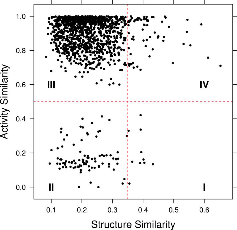
where Act(A) and Act(B) are the activities of compounds A & B and Actmax and Actmin are the maximum and minimum activities respectively. The resultant plot can be divided into four quadrants (Figure 1), allowing one to identify molecules characteristic of one of four possible behaviors: smooth regions of the SAR space, (rough) activity cliffs, non-descript (i.e., low structural similarity and low activity similarity) and scaffold hops (low structural similarity but high activity similarity). Maggiora and Shanmugasundaram then describe the application of information theoretic methods such as entropy calculations to qualitatively assess the degree of information possessed by pairs of compounds in different regions of the SAS plot. One drawback of SAS maps (but common to many other techniques that characterize SAR landscapes), is that one must select hard thresholds to divide the map into the four quadrants (though the qualitative identification is independent of the specific thresholds). As a result, thresholds are generally specific to a dataset and representation and thus SAS maps are not always easy to compare across datasets, targets and so on.
Figure 1.
An example of a Structure-Activity Similarity (SAS) map. Quadrants I, II, III and IV correspond to rough regions (activity cliffs), non-descript regions, scaffold hops and smooth regions of an activity landscape, respectively. The map was generated for a random subset of 50 compunds taken from the GSK malaria dataset [41]. Structure similarity was evaluated using CDK [42] hashed fingerprints and the Tanimoto metric.
One of the drawbacks of the SAS approach is that it is based on a 2-D plot that, in general, requires manual inspection. A more flexible approach is to develop a single measure that can characterize the presence or absence of an activity cliff (though more strictly, one should speak of the “degree of a cliff”). Guha and Van Drie [12] described the Structure Activity Landscape Index (SALI):
| (2) |
where Ai and Aj are the observed activities of the i'th and j'th molecules and sim(i, j) is the similarity between the two molecules. Note that this formulation assumes similarities range from 0 to 1 and is based on the use of the Tanimoto similarity metric. The SALI represents a pairwise measure of the extent to which a pair of molecule exhibits an activity cliff - larger values indicate the pair is a bigger cliff. The original work by Guha and Van Drie employed hashed fingerprints to evaluate molecular similarity and showed that the analysis was independent of the similarity metric employed. Later Guha [13] highlighted the use of different structural representations (continuous descriptors and even fit parameters from dose response curves) and their effects on SALI calculations.
An alternative formulation is the SAR Index (SARI) devised by Peltason and Bajorath [14] and is defined for a pair of molecules as
| (3) |
where the continuity score (scorecont) is derived from the potency weighted mean of the similarity between the two molecules and the discontinuity score (scoredisc) is the product of the average potency difference between pairs and pairwise ligand similarities. One of the key differences between the SALI and SARI formulations is that the former focuses on individual pairs of molecules, independent of targets whereas the SARI address groups of molecules for a given target and allows a direct identification of continuous and discontinuous SAR trends vis a vis specific targets.
3 SAR Landscape Visualization
The previous section highlighted multiple approaches to numerically charactering SAR landscapes and activity cliffs. Naturally, there are multiple ways of viewing such data. The SAS map (Figure 1) previously mentioned is one such approach and is a direct visualization of activity similarity versus structural similarity. One benefit is that one can divide the plot into four regions and focus on specific groups of molecules in a direct fashion (i.e., there is no abstraction involved). Recently, Yongye et al [15] have extended the SAS maps, to replace the structural similarity axis with property similarities. They noted that such PAS maps were more disperse compared to the traditional SAS maps, but provided much of the same information as them. They also considered combining all three - structure, property and acitivity into a single 3D plot, termed the SPA map - which maintains much of the features of SAS and PAS maps, but do require a more interactive visualization to be useful.
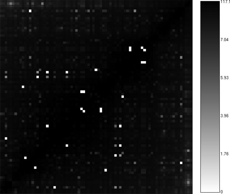
Guha and Van Drie [12] have described multiple approaches to the visualization of SALI values. For a set of molecules which have been analyzed using the SALI method, the simplest visualization is to directly plot the SALI matrix as an image, as shown in Figure 2 for a collection of 79 PDGFR inhibitors [16]. Usually, the X and Y axes will be ordered so that less active molecules are located towards the origin. In such a representation one can identify two classes of molecule pairs - those in which one molecule is less potent and the other highly potent and those cases where both molecules are more potent. The former is an example of a true activity cliff, and the main focus of this type of analysis. The latter represents cases that are technically not activity cliffs, even though, based on Equation 3 they are identified as such; instead they can be regarded as isosteric equivalents and suggest scenarios where small functional group changes more or less maintain the observed potency. Usually, these matrices are color coded; in this case, light blocks represent large SALI values and darker blocks represent smaller SALI values. While a useful summary of the SALI analysis of a dataset, the SALI matrix heatmap visualization is somewhat crude - though when used in conjunction with interactive graphics can be useful to quickly zoom in on to candidate activity cliffs.
Figure 2.
A heatmap representation of the SALI matrix for a set of 79 PDGFR inhibitors, using CDK hashed fingerprints and the Tanimoto metric. The axes are ordered such that lesst active molecules are located towards the origin. The color bar indicates the range of SALI values for this dataset.
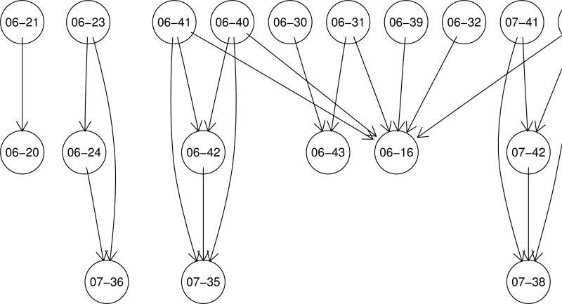
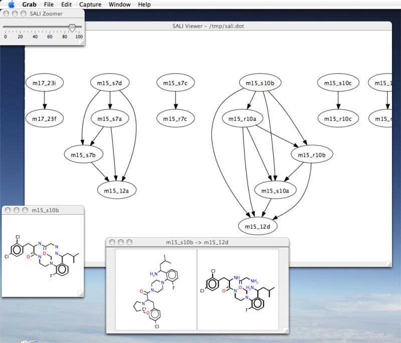
An alternative to the visualization of the SALI matrix is the SALI network, which is derived from the SALI matrix by choosing a user specifed threshold (usually a percentage of the maximum SALI value for the dataset) and selecting pairs whose SALI value is greater than the threshold. Each member of a pair becomes a node and the two nodes are connected by an edge. This results in a network represention as shown in Figure 3. Clearly, at very high thresholds, only the most significant cliffs are identified and the network is sparse. At lower thresholds, many pairs are accepted and we obtain a much more complex (and difficult to navigate) network. While such network visualizations are interesting, static pictures do not convey the utility. As a result the authors developed an interactive application (Figure 4) that lets one generate these networks and vary the threshold dynamically, allowing to smoothly transition from a hairball where every molecule is connected to every other molecule to a more sparse network that focuses only on the most significant cliffs.
Figure 3.
A SALI network visualization for a set of 62 glucocorticoid inhibitors [3, 2], generated using a SALI threshold of 30% of the maximum SALI value for this dataset. Each node represents a compound and an edge is drawn if the SALI value for the pair of compounds was greater than the threshold.
Figure 4.
A screenshot of the SALI Viewer app (http://sali.rguha.net), developed by Guha and Van Drie to generate and interact with SALI networks
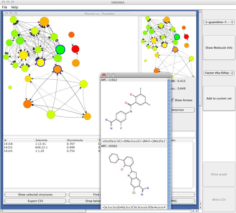
A somewhat related approach described by Wawer et al [17] was the concept of network-like similarity graphs (NSG). This representation first draws a network where the active compounds are nodes and two nodes are connected by an edge if their similarity is greater than some user specified threshold. Nodes are colored based on their potency and scaled based on their local discontinuity score [14] of the compound. The authors note that the NSG representation was designed to multiplex information - ranging from pairwise similarity relationships and compound clusters to SAR discontinuity, activity cliffs and identifying different SAR regions within a dataset. Recently, Lounkine et al [18] published the SARANEA tool that allows one to evaluate SAR landscapes based on SARI and NSG's (Figure 5) and supports interactive clustering and exploration of the resultant networks. A modification of the NSG concept ws described by Iyer et al [19], in which mechanism of action (MoA) were also taken into account in the construction of an NSG. In this approach, the NSG was initially constructed based on the usual similarity considerations. Subsequent discontinuity scores were then calculated separately for subsets of compounds with similar MoA's. With the inclusion of MoA information, the authors show how they can be used to identify distinct compound series with similar MoA's as well identifying similar series with different MoA's (thus leading to the concept of “mechanism hopping” by analogy with the idea of scaffold hopping).
Figure 5.
A screenshot of the SARANEA application by Loukine et al [18] to explore SAR datasets based on the SARI metric and network structure graphs.
Seebeck et al [20] developed a novel visualization based on the idea of SALI, but abstracted to consider both ligand and receptor. Based on this abstraction they were able to identify hotspots within a protein binding site that are likely responsible for causing activity cliffs. Based on their analysis they were able to rank protein atoms in terms of the frequency by which they are identified as hotspots, thus providing an intuitive map of the binding site in terms of activity cliff occurrence. While this visualization is not a direct representation of the landscape itself, it is clearly an important alternative to the purely ligand based visualizations described above.
4 Applications
Since its articulation in 2006 by Maggiora [4], there have been a number of extensions and applications of the landscape concept in various areas of SAR analysis. Many applications focus on the role of activity cliffs in compound class specific or target specific collections. For example, Wasserman and Bajorath report a systematic study of chemical substitutions that lead to the formation of an activity cliff [21] in various compound classes. Hu and Bajorath [22] studied scaffolds as an alternative grouping of compounds and identified scaffolds that exhibit a propensity for activity cliff formation. Given that activity cliffs are derived from specific ligand-receptor interactions, target specificity (i.e., selectivity) of activity cliffs is an obvious focus of analysis. Peltason et al [23] describe an approach to studying “structure-selectivity relationships” (SSR's) using NSG's and SARI values, leading to the concept of “selectivity cliffs”, structurally related compounds that exhibit large differences in selectivity. Another interesting extension to activity cliffs is the idea of activity ridges. In contrast to activity cliffs, which characterize single points on an activity landscape, activity ridges arise when one considers “. . . overlapping combinatorial activity cliffs between participating compounds . . . ” [24]. In other words, an activity ridge is said to occur when multiple compounds in a series form activity cliffs (possibly with each other). Wawer et al [25] have extended the idea of NSG's to to identifying local SAR trends in large high throughput screening datasets. By identifying paths in the NSG that connect regions of low and high SAR discontinuity, the authors were able to identify “SAR pathways” - sequences of compounds, along which one can observe continuous SAR changes. The reader is referred to Wasserman et al [26] who provide a detailed summary of many applications. In the following sections we discuss a few selected applications of the landscape concept in the context of predictive models and feature selection.
4.1 Landscapes and model quality
Predictive models are ubiquitious in computational drug discovery and the literature is replete with models for a variety of biological endpoints. Models can be broadly divided into two groups: statistical or mathematical models (such as linear regression, random forests and SVMs) and physical models (such as docking and pharmacophore approaches). Key to the development and use of such models are metrics to measure their quality and performance. Examples include correlation coefficients (R2), root mean square error, q2, root mean square deviation and so on. But more fundamentally, the goal of any predictive model, irrespective of the underlying methodology, is to capture (or encode) the SAR landscape. Thus one approach to quantifying model quality is to measure how well a model has encoded the landscape. Guha and Van Drie [27] have described such an approach, based on how well a model predicts the ordering of nodes in the edges of a SALI network at varying SALI cutoffs. While statistical models will provide a predicted activity, this approach merely asks whether molecule A is predicted to be more potent than molecule B (assuming A & B form an edge in the SALI network). This procedure is repeated for differing SALI thresholds. At a high threshold, the approach focuses on whether the model can predict orderings for the most significant cliffs. Whereas at lower thresholds, the approach measures the ability of the model to capture the orderings of the bulk dataset. In the extreme (threshold of 0), the approach is equivalent to evaluating Kendalls τ on the predicted vs observed values. The procedure allows one to draw a curve of (normalized) number of edges correctly predicted versus the SALI threshold. By evaluating the area under the curve (termed the SALI Curve Index or SCI), one obtains a single number characterizing the models’ quality. A model that predicts all orderings correctly, at all SALI thresholds would have a SCI = 1.0 (and a curve that is horizontal at 1.0). In reality most models will not correctly predict all edge orderings and we expect poorer performance on the edges corresponding to significant activity cliffs. However, the authors note that physical models, that are able to directly account for the physical basis of activity cliffs (by virtue of including receptor information) do perform significantly better (with SCI > 0.9). But more importantly, the approach is able to measure and compare model quality for fundamentally different types of models, which in addition may output different things. That is, one can compare say a docking model and a random forest model based on their SCI values, even though one predicts binding energies and one activities. In contrast, the traditional metrics for these two models (RMSD and out-of-bag error) are not directly comparable.
4.2 Consensus approaches
One of the key features of any characterization of activity landscapes is that a structure representation must be selected a priori. It is well known from QSAR studies and analyses of chemical spaces, that relationships in one chemical space (i.e., one structure representation) do not necessarily carry over into another chemical space. Thus is it can be expected that activity cliffs identified on the basis of a certain structural representation (say, fingerprints) will not be considered activity cliffs in another representation (say, 2D topological descriptors) [28]. One approach to identifying representation independant activity cliffs is to use a consensus approach as described by Medina-Franco et al [29] and Yongye et al [15]. These approaches are extensions of the data fusion techniques described by Whittle et al [30, 31]. For example, Medina-Franco et al employ a mean fusion rule applied to SALI values ontained using multiple 2D (MACCS keys, typed graph distances and circular fingerprints) and 3D representations (based on single conformers and ROCS similarities). They also generated SAS maps based on different structural representations. In all cases, the goal was to identify those pairs of molecules that were considered activity cliffs in the majority of the representations. Such pairs were termed “consensus activity cliffs” and can be considered “true” cliffs, that are not dependent on the structural representation being employed. Based on the SAS map approach, a compound pair was regarded as a consensus activity cliff if it was located in the lower right quadrant in the majority of representations. They quantitated this by defining a degree of consensus (DoC). The authors also noted that results obtained from the fusion of SALI values using 2D and 3D representations corresponded to those based on the SAS map analysis. In their follow on work, Yongye et al [15] investigated the use of multiple conformers, though they note that in most cases the bioactive conformer is usually unknown and thus multi-conformer landscape analyses are still open for exploration.
One of the key features of consensus approaches is not to identify the “best” representation. Instead, the focus is on employing multiple representations to identify pairs that behave consistently as activity cliffs. Both studies also highlighted the fact that even though individual similarity measures were not necessarily well correlated, when combined they were useful in terms of identifying consensus cliffs. They also noted that in general, 2D methods showed a better degree of consensus than 3D methods - though this may have been due to no conformers (or when conformers were considered, insufficient sampling of conformer space).
4.3 Feature selection and landscapes
Given that identifying a pair of molecules as an activity cliff is dependent on their representation (fingerprints, 2D or 3D descriptors), approaches such consensus methods described in the previous section play a role in identifying “true” (i.e., representation independent) activity cliffs.
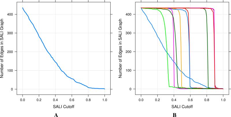
However, given that a representation essentially defines a landscape, one can ask: which structural representation leads a to a good activity landscape?. The problem is that it is difficult to define what is a “good” landscape. One view taken by this author, is that a good landscape is somewhere between a smooth (minimal activity cliffs) and a very rough one. The former represents minimal variation in activity with structural changes whereas the latter represents large changes in activity with every change in structure. Neither are amenable for SAR analysis or modeling and do not provide useful information. One way to measure the smoothness of the landscape is to count the edges in a SALI network at a given threshold. By plotting the edge count versus the cutoff, one obtains a curve. Such a curve that smoothly decreases with increasing SALI threshold could be suggestive of a good landscape. On the other hand, a curve that is steep at either low or high threshold would be indicative of a extreme rough or extreme smooth landscape. By evluating the area under this curve, one could use it to identify a structural representation that represents a “good” landscape. Figure 6 displays examples of these curves for different structural representations. Figure 6B highlights the fact that for many 2D representations, the landscapes are either overly smooth or overly jagged.
Figure 6.
Characterizing the smoothness of activity landscapes, by counting edges in the SALI network at varying SALI thresholds. A is derived from a binary fingerprint representation and appears to represent a “good” landscape. B represents curves from randomly selected 2D 4-descriptor representations. In general these representations lead to overly smooth or overly jagged landscapes. The light blue line represents the curve obtained from the fingerprint representation.
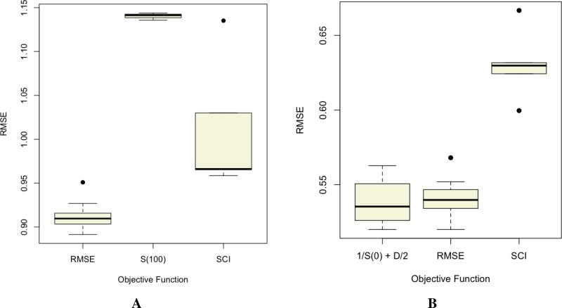
Another aspect of feature selection is the problem of model identification - choosing a single (or few) model that accurately encodes the activity landscape. Based on the discussion of the SCI in Section 4.1, a convenient approach is to use the SCI (and curve) as part of an objective function in traditional feature selection algorithms [32] (genetic algorithms, simulated annealing and so on). Thus one could define an objective function that simply maximizes the SCI value. An alternative function is to ensure that the model correctly predicts the bulk of the dataset (i.e., maximize the value of the curve at a threshold of 0) and correctly predicts the most significant activity cliff (i.e., maximize the value of the curve at a threshold of 1.0). But it is also important to note that for most statistical models, activity cliffs appear as outliers [13]. Thus an objective function that attempts to maximize the the correct prediction of activity cliffs, will invariably lead to a model that is overfit. As a result, activity cliff-based objective functions should take into account some measure of generalizability. However, it is not always clear when an activity landscape based feature selection procedure outperforms traditional approachs (such as based on RMSE). Figure 7 displays the distribution of RMSE values for the top 10 models identified using a genetic algorithm with different objective functions. Figure 7A employed the Sutherland et al [33] benzodiazepine dataset and in this case, it is clear that the traditional RMSE based objective function obtains the best set of models. S(100) which maximizes the the models ability to capture activity cliffs (irrespective of everything else) performs poorest, as expected. Interestingly, the SCI based function shows a wider spread of model performances. Figure 7B is based on a set of ER-β ligands [34] and in this case we see that a landscape based objective function (1/S(0) + D/2, where S(0) is the value of the SALI curve at a threshold of 0 and D is the difference between the value of the SALI curve at a threshold of 0 and threshold of 1) does slightly better than the RMSE based function, though the former does show a wider spread of model performances. Once again, an objective function that simply maximizes the area under the SALI curve (SCI) leads to poorer performance (likely due to overfitting). The key point of this is that, a priori it is difficult to determine when a landscape based objective function outperforms traditional functions based on statistical measures of model quality.
Figure 7.
Distribution of root mean square error (RMSE) for the top 10 linear regression models obtained using a genetic algorithm with different objective functions. A was based on the Sutherland benzodiazepine dataset [33] and B was based on the Malamas dataset [34] of ER-β ligands.
4.4 Predicting the landscape
While it is useful to consider retrospective analyses of SAR datasets using the methods here, prospective applications could play an important role by explicitly taking into account the structure of the landscape at various stages of the drug discovery pipeline (hit selection, lead optimization and so on). Currently, there are few examples of prospective applications. Guha [35] has described an approach based on the prediction of SALI values. The method considers the n(n – 1)/2 pairwise SALI values derived from a dataset of n molecules as the dependent variable. The independent variables are defined in terms of a function, fagg, which takes the descriptor values for the original pair of molecules and returns a descriptor vector of equal length, that is an aggregation of the original pair of descriptor values. The simplest such function is the arithmetic mean of the original descriptor value pairs. Finally, a predictive model is developed to predict the pairwise SALI values from the aggregated descriptor values. It is interesting to note that this approach is even applicable to small datasets since the model is based on the pairwise values (thus a 15 molecule dataset leads to a 105 observation dataset for the SALI predictions). While it is not expected that the model predicts the most significant activity cliffs (since they still behave as outliers in the pairwise approach), initial results have indicated that prediction of SALI values is feasible.
Seebeck et al [20] have described an approach, based on SALI, that takes into account both ligand and receptor features that allow them to develop pharmacophore hypotheses, based on the structure of the SAR landscape. In their method, termed Identification of Structrure-based Activity Cliffs (ISAC). Their approach considers protein-ligand interaction energies as descriptors, allowing them to avoid an explicit dependence on ligand structure and specific functional groups. As Seebeck et al [20] note: “. . . structurally different ligands with similar potencies, which can be explained by similar interaction profiles, are captured by the ISAC approach.”. Based on the ISAC methodology, they were able to derive a set of target specific scoring models [36] and pharmacophoric constraints, which were then applied to several structure based virtual screens. Their results indicate that inclusion of activity cliff hotspot information as captured by ISAC led to a significant improvement in hit rates and enrichments, compared to traditional scoring functions. In a sense, the ISAC approach is a prediction of the landscape, using an alternative route; rather the work with only ligand information, the authors employ protein and ligand information to predict active compounds.
5 Conclusions
It is important to remember that an activity cliff, in general, arises due to a key interaction between a specific feature of a small molecule and the receptor. Thus the activity cliff concept and associated analyses cannot be applied to bulk properties such as solubility (though a number of activity cliff-like cases can be found in large collections of solubility data [37]). In many cases, these key ligand-receptor interactions can be elucidated via other means, and thus could be used to identify activity cliffs prospectively. However, it is also the case that the receptor structure may not be known and then, prospective analyses of activity cliffs could provide insight into pharmacophoric features that represent key ligand-receptor interactions. Thus purely ligand based approaches can be limiting. Methods that take into account ligand and receptor [20] clearly capture more information and can play a prospective role.
One of the main limitations of the landscape concept and associated concepts such as activity cliffs and NSG's is that they all require a pairwise analysis of the dataset. Thus, most algorithms referenced in this work do not scale to tens of thousands of compounds. Indeed, Wawer et al [25] employed high throughput screening (HTS) data to identify activity cliffs and SAR pathways. Yet, the largest dataset employed was just 2,434 compounds. One way to address this problem of dataset size is to prefilter large datasets (e.g., only consider actives from a HTS campaign), or employ some form of sampling. A number of approaches described by Bajorath and co-workers make use of the local neighborhood of reference compounds. In such cases, fast (or even approximate) near neighbor search algorithms [38, 39, 40] would significantly speed up such analyses.
It is clear that the landscape paradigm has stimulated the cheminformatics community to develop a wide variety of analytical and visual approaches to quantifying and characterizing SAR data. Multiple numerical formulations of activity cliffs have been devised and a variety of applications of these definitions have been investigated, ranging from the determination of “SAR pathways” to selectivity cliffs. In the area of visualization, one of the key outcomes of the landscape view is the development of a variety of network visualizations. While such networks have become nearly ubiquitious in many areas of science, many such depictions do not necessarily lead to novel conclusions. While it still remains to be seen, whether chemical structure networks developed on the basis of the SAR landscape view provide real insight (beyond that which could be obtained from traditional tabular summaries or clustering methods), these appproaches to represent a step forward in the visual summarization of structure-actvity data.
References
- 1.Martin YC, Kofron JL, Traphagen LM. Do Structurally Similar Molecules Have Similar Biological Activity?. J. Med. Chem. 2002;45:4350–4358. doi: 10.1021/jm020155c. [DOI] [PubMed] [Google Scholar]
- 2.Takahashi H, Bekkali Y, Capolino AJ, Gilmore T, Goldrick SE, Nelson RM, Terenzio D, Wang J, Zuvela-Jelaska L, Proudfoot J, Nabozny G, Thomson D. Discovery and SAR Study of Novel Dihydroquinoline Containing Glucocorticoid Receptor Ligands. Bioorg. Med. Chem. Lett. 2006;16:1549–1552. doi: 10.1016/j.bmcl.2005.12.043. [DOI] [PubMed] [Google Scholar]
- 3.Takahashi H, Bekkali Y, Capolino AJ, Gilmore T, Goldrick SE, Kaplita PV, Liu L, Nelson RM, Terenzio D, Wang J, Zuvela-Jelaska L, Proudfoot J, Nabozny G, Thomson D. Discovery and SAR Study of Novel Dihydroquinoline Containing Glucocorticoid Receptor Agonists. Bioorg. Med. Chem. Lett. 2007;17:5091–5095. doi: 10.1016/j.bmcl.2007.07.021. [DOI] [PubMed] [Google Scholar]
- 4.Maggiora GM. On Outliers and Activity Cliffs–Why QSAR Often Disappoints. J. Chem. Inf. Model. 2006;46:1535–1535. doi: 10.1021/ci060117s. [DOI] [PubMed] [Google Scholar]
- 5.Leach A, Jones H, Cosgrove D, Kenny P, Ruston L, MacFaul P, Wood J, Colclough N, Law B. Matched Molecular Pairs as a Guide in the Optimization of Pharmaceutical Properties; a Study of Aqueous Solubility, Plasma Protein Binding and Oral Exposure. J. Med. Chem. 2006;49:6672–6682. doi: 10.1021/jm0605233. [DOI] [PubMed] [Google Scholar]
- 6.Keefer CE, Chang G, Kauffman GW. Extraction of Tacit Knowledge from Large ADME Data Sets via Pairwise Analysis. Bioorg. Med. Chem. 2011;19:3739–3749. doi: 10.1016/j.bmc.2011.05.003. [DOI] [PubMed] [Google Scholar]
- 7.Warner DJ, Griffen EJ, St-Gallay SA. WizePairZ: A Novel Algorithm to Identify, Encode, and Exploit Matched Molecular Pairs with Unspecified Cores in Medicinal Chemistry. J. Chem. Inf. Model. 2010;50:1350–1357. doi: 10.1021/ci100084s. [DOI] [PubMed] [Google Scholar]
- 8.Hajduk PJ, Sauer DR. Statistical Analysis of the Effects of Common Chemical Substituents on Ligand Potency. J. Med. Chem. 2008;51:553–564. doi: 10.1021/jm070838y. [DOI] [PubMed] [Google Scholar]
- 9.Sheridan RP, Hunt P, Culberson JC. Molecular Transformations as a Way of Finding and Exploiting Consistent Local QSAR. J. Chem. Inf. Model. 2006;46:180–192. doi: 10.1021/ci0503208. [DOI] [PubMed] [Google Scholar]
- 10.Agrafiotis D, Shemanarev M, Connolly P, Farnum M, Lobanov V. SAR Maps: A New SAR Visualization Technique for Medicinal Chemists. J. Med. Chem. 2007;50:5926–5937. doi: 10.1021/jm070845m. [DOI] [PubMed] [Google Scholar]
- 11.Shanmugasundaram V, Maggiora G. CINF-032. 222nd ACS National Meeting, Chicago, IL, United States. American Chemical Society; Washington, D.C.: 2001. Characterizing Property and Activity Landscapes Using an Information-Theoretic Approach. [Google Scholar]
- 12.Guha R, Van Drie J. The Structure-Activity Landscape Index: Identifying and Quantifying Activity-Cliffs. J. Chem. Inf. Model. 2008;48:646–658. doi: 10.1021/ci7004093. [DOI] [PubMed] [Google Scholar]
- 13.Guha R. Cheminformatics and Computational Chemical Biology. In: Bajorath J, editor. Chapter The Ups and Downs of Structure-Activity Landscapes. Springer; Berlin, Germany: 2010. [Google Scholar]
- 14.Peltason L, Bajorath J. SAR Index: Quantifying the Nature of Structure-Activity Relationships. J. Med. Chem. 2007;50:5571–5578. doi: 10.1021/jm0705713. [DOI] [PubMed] [Google Scholar]
- 15.Yongye AB, Byler K, Santos R, Martínez-Mayorga K, Maggiora GM, Medina-Franco JL. Consensus Models of Activity Landscapes with Multiple Chemical, Conformer, and Property Representations. J. Chem. Inf. Model. 2011;51:1259–1270. doi: 10.1021/ci200081k. [DOI] [PubMed] [Google Scholar]
- 16.Pandey A, Volkots DL, Seroogy JM, Rose JW, Yu J-C, Lambing JL, Hutchaleelaha A, Hollenbach SJ, Abe K, Giese NA, Scarborough RM. Identification of Orally Active, Potent, and Selective 4-Piperazinylquinazolines as Antagonists of the Platelet-Derived Growth Factor Receptor Tyrosine Kinase Family. J. Med. Chem. 2002;45:3772–3793. doi: 10.1021/jm020143r. [DOI] [PubMed] [Google Scholar]
- 17.Wawer M, Peltason L, Weskamp N, Teckentrup A, Bajorath J. Structure-Activity Relationship Anatomy by Network-like Similarity Graphs and Local Structure-Activity Relationship Indices. J. Med. Chem. 2008;51:6075–6084. doi: 10.1021/jm800867g. [DOI] [PubMed] [Google Scholar]
- 18.Lounkine E, Wawer M, Wassermann AM, Bajorath J. SARANEA: A Freely Available Program to Mine Structure-Activity and Structure-Selectivity Relationship Information in Compound Data Sets. J. Chem. Inf. Model. 2010;50:68–78. doi: 10.1021/ci900416a. [DOI] [PubMed] [Google Scholar]
- 19.Iyer P, Stumpfe D, Bajorath J. Molecular Mechanism-Based Network-Like Similarity Graphs Reveal Relationships Between Different Types of Receptor Ligands and Structural Changes that Determine Agonistic, Inverse-Agonistic, and Antagonistic Effects. J. Chem. Inf. Model. 2011;51:1281–126. doi: 10.1021/ci2001378. [DOI] [PubMed] [Google Scholar]
- 20.Seebeck B, Wagener M, Rarey M. From Activity Cliffs to Target-Specific Scoring Models and Pharmacophore Hypotheses. ChemMedChem. 2011 doi: 10.1002/cmdc.201100179. in press. [DOI] [PubMed] [Google Scholar]
- 21.Wassermann AM, Bajorath J. Chemical Substitutions that Introduce Activity Cliffs Across Different Compound Classes and Biological Targets. J. Chem. Inf. Model. 2010;50:1248–1256. doi: 10.1021/ci1001845. [DOI] [PubMed] [Google Scholar]
- 22.Hu Y, Bajorath J. Molecular Scaffolds with High Propensity to Form Multi-Target Activity Cliffs. J. Chem. Inf. Model. 2010;50:500–510. doi: 10.1021/ci100059q. [DOI] [PubMed] [Google Scholar]
- 23.Peltason L, Hu Y, Bajorath J. From Structure-Activity to Structure-Selectivity Relationships: Quantitative Assessment, Selectivity Cliffs, and Key Compounds. ChemMedChem. 2009;4:1864–1873. doi: 10.1002/cmdc.200900300. [DOI] [PubMed] [Google Scholar]
- 24.Vogt M, Huang Y, Bajorath J. From Activity Cliffs to Activity Ridges: Informative Data Structures for SAR Analysis. J. Chem. Inf. Model. 2011;51:1848–1856. doi: 10.1021/ci2002473. [DOI] [PubMed] [Google Scholar]
- 25.Wawer M, Peltason L, Bajorath J. Elucidation of Structure-Activity Relationship Pathways in Biological Screening Data. J. Chem. Inf. Model. 2009;52:1075–1080. doi: 10.1021/jm8014102. [DOI] [PubMed] [Google Scholar]
- 26.Wassermann AM, Wawer M, Bajorath J. Activity Landscape Representations for Structure-Activity Relationship Analysis. J. Med. Chem. 2010;53:8209–8223. doi: 10.1021/jm100933w. [DOI] [PubMed] [Google Scholar]
- 27.Guha R, Van Drie J. Assessing How Well a Modeling Protocol Captures a Structure-Activity Landscape. J. Chem. Inf. Model. 2008;48:1716–1728. doi: 10.1021/ci8001414. [DOI] [PubMed] [Google Scholar]
- 28.Peltason L, Iyer P, Bajorath J. Rationalizing Three-Dimensional Activity Landscapes and the Influence of Molecular Representations on Landscape Topology and the Formation of Activity Cliffs. J. Chem. Inf. Model. 2010;50:1021–1033. doi: 10.1021/ci100091e. [DOI] [PubMed] [Google Scholar]
- 29.Medina-Franco JL, Martínez-Mayorga K, Bender A, Marín RM, Giulianotti MA, Pinilla C, Houghten RA. Characterization of Activity Landscapes Using 2D and 3D Similarity Methods: Consensus Activity Cliffs. J. Chem. Inf. Model. 2009;49:477–491. doi: 10.1021/ci800379q. [DOI] [PubMed] [Google Scholar]
- 30.Whittle M, Gillet VJ, Willett P, Loesel J. Analysis of Data Fusion Methods in Virtual Screening: Similarity and Group Fusion. J. Chem. Inf. Model. 2006;46:2206–2219. doi: 10.1021/ci0496144. [DOI] [PubMed] [Google Scholar]
- 31.Whittle M, Gillet VJ, Willett P, Loesel J. Analysis of Data Fusion Methods in Virtual Screening: Theoretical Model. J. Chem. Inf. Model. 2006;46:2193–2205. doi: 10.1021/ci049615w. [DOI] [PubMed] [Google Scholar]
- 32.Kohavi R, John G. Wrappers for Feature Subset Selection. Artif. Intell. 1997;97:273–324. [Google Scholar]
- 33.Sutherland J, O'Brien L, Weaver D. Spline-Fitting with a Genetic Algorithm: A Method for Developing Classification Structure-Activity Relationships. J. Chem. Inf. Comput. Sci. 2003;43:1906–1915. doi: 10.1021/ci034143r. [DOI] [PubMed] [Google Scholar]
- 34.Malamas MS, Manas ES, McDevitt RE, Gunawan I, Xu ZB, Collini MD, Miller CP, Dinh T, Henderson RA, Keith JC, Jr, Harris HA. Design and Synthesis of Aryl Diphenolic Azoles as Potent and Selective Estrogen Receptor-Beta Ligands. J. Med. Chem. 2004;47:5021–5040. doi: 10.1021/jm049719y. [DOI] [PubMed] [Google Scholar]
- 35.Guha R. Abstracts of Papers of the American Chemical Society. American Chemical Society; Washington D.C.: 2010. What Makes a Good Structure Activity Landscape?. [Google Scholar]
- 36.Seifert MH. J. Targeted Scoring Functions for Virtual Screening. Drug Discov. Today. 2009;14:562–569. doi: 10.1016/j.drudis.2009.03.013. [DOI] [PubMed] [Google Scholar]
- 37.Guha R, Dexheimer TS, Kestranek AN, Jadhav A, Chervenak AM, Ford MG, Simeonov A, Roth GP, Thomas CJ. Exploratory Analysis of Kinetic Solubility Measurements of a Small Molecule Library. Bioorg. Med. Chem. 2011;19:4127–4134. doi: 10.1016/j.bmc.2011.05.005. [DOI] [PMC free article] [PubMed] [Google Scholar]
- 38.Dutta D, Guha R, Jurs P, Chen T. Scalable Partitioning and Exploration of Chemical Spaces using Geometric Hashing. J. Chem. Inf. Model. 2006;46:321–333. doi: 10.1021/ci050403o. [DOI] [PubMed] [Google Scholar]
- 39.Arya S, Mount D, Netanyahu N, Silverman R, Wu A. An Optimal Algorithm for Approximate Nearest Neighbor Searching in Fixed Dimensions. J. ACM. 1998;45:891–923. [Google Scholar]
- 40.Kim B, Park S. A Fast K Nearest Neighbor Finding Algorithm Based on the Ordered Partition. PAMI. 1986;8:761–766. doi: 10.1109/tpami.1986.4767859. [DOI] [PubMed] [Google Scholar]
- 41.Gamo F-J, Sanz LM, Vidal J, de Cozar C, Alvarez E, Lavandera J-L, Vanderwall DE, Green DVS, Kumar V, Hasan S, Brown JR, Peishoff CE, Cardon LR, Garcia-Bustos JF. Thousands of Chemical Starting Points for Antimalarial Lead Identification. Nature. 2010;465:305–310. doi: 10.1038/nature09107. [DOI] [PubMed] [Google Scholar]
- 42.Steinbeck C, Hoppe C, Kuhn S, Floris M, Guha R, Willighagen E. Recent Developments of the Chemistry Development Kit (CDK) - An Open-Source Java Library for Chemoand Bioinformatics. Curr. Pharm. Des. 2006;12:2110–2120. doi: 10.2174/138161206777585274. [DOI] [PubMed] [Google Scholar]


