Dimensionality and noise in energy selective x-ray imaging

Abstract

Purpose: To develop and test a method to quantify the effect of dimensionality on the noise in energy selective x-ray imaging.

Methods: The Cramèr-Rao lower bound (CRLB), a universal lower limit of the covariance of any unbiased estimator, is used to quantify the noise. It is shown that increasing dimensionality always increases, or at best leaves the same, the variance. An analytic formula for the increase in variance in an energy selective x-ray system is derived. The formula is used to gain insight into the dependence of the increase in variance on the properties of the additional basis functions, the measurement noise covariance, and the source spectrum. The formula is also used with computer simulations to quantify the dependence of the additional variance on these factors. Simulated images of an object with three materials are used to demonstrate the trade-off of increased information with dimensionality and noise. The images are computed from energy selective data with a maximum likelihood estimator.

Results: The increase in variance depends most importantly on the dimension and on the properties of the additional basis functions. With the attenuation coefficients of cortical bone, soft tissue, and adipose tissue as the basis functions, the increase in variance of the bone component from two to three dimensions is 1.4 × 10³. With the soft tissue component, it is 2.7 × 10⁴. If the attenuation coefficient of a high atomic number contrast agent is used as the third basis function, there is only a slight increase in the variance from two to three basis functions, 1.03 and 7.4 for the bone and soft tissue components, respectively. The changes in spectrum shape with beam hardening also have a substantial effect. They increase the variance by a factor of approximately 200 for the bone component and 220 for the soft tissue component as the soft tissue object thickness increases from 1 to 30 cm. Decreasing the energy resolution of the detectors increases the variance of the bone component markedly with three dimension processing, approximately a factor of 25 as the resolution decreases from 100 to 3 bins. The increase with two dimension processing for adipose tissue is a factor of two and with the contrast agent as the third material for two or three dimensions is also a factor of two for both components. The simulated images show that a maximum likelihood estimator can be used to process energy selective x-ray data to produce images with noise close to the CRLB.

Conclusions: The method presented can be used to compute the effects of the object attenuation coefficients and the x-ray system properties on the relationship of dimensionality and noise in energy selective x-ray imaging systems.

INTRODUCTION

With the Alvarez-Macovski¹ approach to energy selective x-ray imaging, we approximate the attenuation coefficient with a linear combination of functions of energy. The number of functions required, the dimensionality, is an important quantity because it determines both the available information and the complexity of the measurements required to extract it. Two functions are most commonly used because they provide good accuracy and can be extracted with two x-ray spectra but it was realized¹ that the dimension was an empirical choice. It depended on the physical properties of x-ray attenuation, the measurement noise and on the state of the art of x-ray detectors. Recently, the count rate capabilities of photon counting detectors have improved so it may be possible to use them in diagnostic imaging.^{2, 3} These detectors have the potential to make measurements with high energy resolution by using pulse height analysis (PHA) and this increased resolution may allow us to extract higher dimensionality information.

The higher dimension information could have important clinical applications. For example, with a two function basis set we are limited to imaging two tissue types such as bone or soft tissue separately. A third material such as adipose tissue cannot be imaged separately but will appear to be a combination of the two basis materials. Addition of a third dimension would allow adipose tissue to be imaged independently in mammography or improve the accuracy of bone densitometry when there are variations in overlying tissues with adipose components. Higher dimension processing can also be used to image externally administered high atomic number contrast agents independent of body structures.

There are several important physical constraints on dimensionality.^{4, 5, 6} The mixture rule states that since x-ray photon energies, which are of the order of 10⁵ electron-volts, are so much greater than chemical binding energies, which are of order 1 electron-volt, x-ray interactions are essentially independent of the chemical state of the atoms. With this approximation, the dimensionality is limited to the number of different elements present in the object in significant quantities. Another constraint is the sum rule for x-ray cross-sections. In the diagnostic energy region, x-rays interact with matter through only a small number of independent physical processes, principally Compton scattering, photoelectric interactions, Rayleigh scattering, and possibly pair-production at high energies. The sum rule states that since the processes are independent the total cross-section is the sum of the individual cross sections. If these cross sections were separable into atomic number dependent and x-ray energy dependent functions, then the dimensionality would be limited to the number of significant interaction processes. Logarithmic plots of these cross sections as a function of energy⁴ for different elements show that they are close to but not exactly parallel.

These physical considerations indicate that the two function basis set commonly used is an empirical choice adopted as a compromise of approximation accuracy, noise versus patient dose considerations, and x-ray imaging systems technology. To consider the potential of photon counting detectors with PHA for increased dimensionality, we need a method to quantify the additional photon numbers, dose, and the improvements in detector system electronic noise and accuracy that are required to extract it. The development and testing of such a method is the purpose of this paper.

The method is based on statistical estimator theory.^{7, 8, 9} This theory was originally developed for analyzing communications systems and it models a system as three parts: a source that produces signals, a transmission channel, and a detector that measures the transmitted signal but adds random noise. For energy selective imaging, the basis functions are known a priori so the basis set coefficients carry all the information. The line integrals of these coefficients completely determine the transmitted spectrum so, in the communications system analogy, they are the signal. The transmission channel is the x-ray source and the attenuation by the body while the detector is a photon counting detector with PHA that measures the energy spectrum of the transmitted radiation. A statistical estimator processes the noisy measurements to give an estimate of the line integrals. These line integrals are summarized as the components of a vector, which is called the A-vector in this paper. The method of computing the A-vector and displaying the information is referred to as A-space processing.

In general, the noise depends on the estimator used. However, estimator theory¹⁰ shows that there is a universal lower limit of the covariance for any nonbiased estimator called the Cramèr-Rao lower bound (CRLB). The CRLB is a fundamental measure that is independent of a particular estimator implementation and is useful as a general metric to characterize the energy selective system performance. It combines the effects of intrinsic dimensionality, which depends on the attenuation coefficients of the materials imaged, with the energy resolution and detector noise to compute the covariance of the A-vector. This covariance determines the image noise, which can be compared with variations in body structures to judge the level required to provide clinically useful information.

An important result from estimator theory¹¹ is that increasing the dimension increases the variance not only of the parameter added but also of all the lower dimension parameters. This paper applies this general result to energy selective systems and shows how the magnitude of the increase depends on factors such as the attenuation coefficient of the additional materials imaged, the source spectrum, and the detector energy resolution. The methods presented allow us to predict the effects of these factors to judge the trade-off between the increased dose required to extract the additional information with satisfactory noise and its clinical utility.

Note that the increase in variance with dimensionality does not imply that energy selective systems are inherently noisier than conventional systems. The A-vector information is a physically different quantity than the data represented by a conventional x-ray image and the noise cannot be directly compared. Indeed, Tapiovaara and Wagner¹² showed theoretically that systems that measure the energy spectrum can have an optimal SNR higher than conventional systems for a given dose. A previous paper¹³ and the results in this paper show that we can use A-space processing with low energy resolution data to produce images with larger signal to noise ratio than conventional photon count or integrated energy images at the same dose. The additional dose that may be required by energy selective systems is used to produce material-selective information. This is an additional information that is not extracted by conventional systems.

Previous studies^{5, 6, 14, 15, 16, 17} concentrated on the “intrinsic dimensionality” of attenuation coefficients. That is, the number of basis functions needed to approximate tabulated attenuation coefficient data with error less than its estimated uncertainty. Alvarez^{5, 6} applied the singular value decomposition (SVD) to determine the approximation error of a table of body material attenuation coefficients as a function of dimensionality. With this approach, the attenuation coefficients of the elements in body materials sampled at a large number of energies are placed in a matrix. The dimensionality is then equal to the rank of this matrix. If the entries in this matrix are considered to be of infinite precision, almost all matrices will have full rank, the smaller of the number of rows or columns. The SVD approximation theorem¹⁸ provides matrices of lower rank that are optimally close to the original matrix. That is, the norm of the difference of the lower rank matrix and the original matrix is minimum for all matrices of that rank. If this norm is less than the estimated accuracy of the attenuation coefficient data, the lower rank can be defined as the intrinsic dimensionality. Roth¹⁹ used the SVD to study the information of three dimension systems that include a high atomic number contrast agent. Weaver and Huddleston¹⁴ used principal components analysis (PCA), which is closely related to the SVD,²⁰ to determine the dimensionality. They compared basis functions based on PCA to the photoelectric effect/Compton scattering¹ and material attenuation coefficient²¹ sets and showed that the principal components provided better accuracy and more stability. Bornefalk¹⁷ also applied PCA with advanced stopping rules and showed that the intrinsic dimensionality of the XCOM attenuation coefficient database may be equal to four.

Gingold and Hasegawa¹⁵ and Williamson et al.¹⁶ not only study the intrinsic dimensionality but also use sensitivity analysis with the partial derivatives of the basis set coefficients to include errors in the measurements. Gingold and Hasegawa compare the errors using two monoenergetic spectra with energies in low and high bands to the sensitivity analysis. Williamson et al. compare the basis vector model with nonlinear parametric models, which approximate the attenuation coefficient based on parameters such as effective atomic number and density. They found that the basis vector models were more promising for dual energy computed tomography systems.

METHODS

In this section, the theory to quantify the dependence of the increased variance on the basis functions, the source spectrum, and the detector energy resolution is developed. Next, Sec. 2E describes simulations of the increased variance using realistic models of the x-ray tube spectrum and the attenuation coefficients of body materials and contrast agents. Finally, in Secs. 2F, 2G, a simulation of images with random noise that illustrates the additional information and the increase in noise with increased dimensionality is described.

Vector data in energy selective systems

The A-space processing analysis is facilitated by using a vector model for the energy selective measurements. In this model, the x-ray attenuation coefficient μ(r, E) at each point r in the object at photon energy E is decomposed using K basis functions as

$$\mu (\mathbf{r},E)=\sum _{k=1}^K{a}_k\left(\mathbf{r}\right)f_k\left(E\right).$$ (1)

If the source produces a photon number spectrum n_source(E), the spectrum transmitted through the object is

$$n_{\text{transmitted}}\left(E\right)=n_{\text{source}}\left(E\right)e^{-{\int }_S\mu (\mathbf{r},E)ds},$$ (2)

where ∫_Sμ(r, E)ds is the integral of the attenuation coefficient on a line from the source to the detector pixel. Introducing the decomposition in Eq. 1, the line integral is

$${\int }_S\mu (\mathbf{r},E)ds=\sum _{k=1}^K{A}_k{f}_k\left(E\right),$$

where A_k = ∫_Sa_k(r)ds. We can summarize the line integrals A_k as the components of a length K vector A = [A₁, A₂, …, A_K]^T, the A-vector. The notation []^T denotes the transpose.

In energy selective imaging, we estimate the A-vector from a set of measurements with different spectra and use this information to compute clinically useful images.¹ Assuming a photon counting detector, the expected values of the measurements are

$$N_j=\int g_j\left(E\right)e^{-{\sum }_{k=1}^K{A}_k\left(\mathbf{r}\right)f_k\left(E\right)}dEj=1...J,$$ (3)

where g_j(E) are the effective spectra for the measurements and J is the number of spectra. As an example, with PHA the effective spectra are g_j(E) = Π_j(E)n_source(E) where Π_j(E) is a rectangle function equal to one in the energy bin and zero otherwise. The model can also be used with switched voltage x-ray tube spectra. Introducing vector notation, the measurements N_j are the elements of a length J vector N = [N₁, N₂, …, N_J]^T. Because of the exponential transmission in Eq. 2, using the logarithm of the data is useful so we introduce the vector $\mathbf{L}=-\log \left(\frac{\mathit{N}}{{\mathbf{N}}_{\mathbf{0}}}\right)$ where N₀ is the vector of “air” values with no object in the system and the quotient notation means corresponding elements of each vector are divided.

The Cramèr-Rao lower bound and dimensionality

Estimator theory shows that there is a lower limit, called the Cramèr-Rao lower bound (CRLB), of the covariance for any nonbiased estimator.¹⁰ As discussed in the Introduction, we can use the CRLB to characterize the energy selective system performance.

The CRLB is the inverse of the Fisher information matrix, F, whose elements are⁸

$$F_{ij}=-⟨\frac{{\partial }^2\log p(\mathbf{L};\mathbf{A})}{\partial A_i\partial A_j}⟩.$$ (4)

In this equation, p(L; A) is the probability density function of the measurements given a particular A-vector and ⟨ ⟩ denotes expected value. The CRLB is the minimum covariance in the sense that the difference of the covariance C_A of any unbiased estimator and the CRLB is positive semidefinite

$${\mathbf{C}}_{\mathbf{A}}-{\mathbf{F}}^{-\mathbf{1}}\ge \mathbf{0}.$$ (5)

Matrix theory²² shows that the diagonal elements of a positive semidefinite matrix are greater than or equal to zero. Therefore, the diagonal elements of the CRLB, which are the variances of the individual components, are the minimum for any unbiased estimator.

Another important result from estimator theory is that adding additional parameters always increases the variance of the estimates or under rare conditions they remain the same.¹¹ For example, if we first use two basis functions and then add an additional function, the variance of the estimates of first two A-vector components with a three function set will be greater than or equal to the variances of the same components with a two function set.

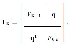
Corollary B.4 of Van den Bos⁹ gives the magnitude of the additional variance. To apply this result, suppose F_{K − 1} is the Fisher matrix with a K − 1 function basis set and ${\mathbf{R}}_{\mathbf{K}-\mathbf{1}}={\mathbf{F}}_{\mathbf{K}-\mathbf{1}}^{-\mathbf{1}}$ is the corresponding CRLB covariance. If we add an additional basis function, then the K dimension Fisher matrix can be partitioned as

(6)

where q is a column vector and F_KK is a scalar. According to the corollary, the CRLB for the K basis function case is

(7)

where the scalar u = F_KK −q^TR_{K − 1}q.

In Eq. 7, the additional covariance due to the added basis function is

$$\mathit{\Delta }{R}_K=\frac{1}{u}{\mathbf{R}}_{\mathbf{K}-\mathbf{1}}{\mathbf{qq}}^{\mathbf{T}}{\mathbf{R}}_{\mathbf{K}-\mathbf{1}}=\frac{1}{u}{\mathbf{vv}}^{\mathbf{T}},$$ (8)

where v = R_{K − 1}q. Since R_{K − 1} is a covariance, it is positive definite so ${\mathbf{R}}_{\mathbf{K}-\mathbf{1}}\mathbf{q}$ is zero if and only if q is equal to zero. Sections 2C, 2D show that q = 0 implies that the additional basis function is orthogonal to the first K − 1 functions. This is usually not the case in energy selective imaging where attenuation coefficients of physical materials are used as basis functions.

The CRLB for an energy selective x-ray imaging system

Since in medical imaging the noise is relatively small, we can use a Taylor's series to derive a linearized approximation about the expected value $⟨\mathbf{A}⟩$

$$\mathbf{L}(⟨\mathbf{A}⟩+\delta \mathbf{A})\approx \mathbf{L}\left(⟨\mathbf{A}⟩\right)+\frac{\partial \mathbf{L}}{\partial \mathbf{A}}\delta \mathbf{A}+\cdots ,$$ (9)

where L is the vector of the logarithm of the measurements described in Sec. 2A. Defining δL = L(⟨A⟩ + δA) − L(⟨A⟩), the linearized model with noise is

$$\delta \mathbf{L}=\mathbf{M}\delta \mathbf{A}+\mathbf{w}.$$ (10)

In this model, M is a matrix with coefficients

$$M_{jk}=-\frac{\partial log\left(N_j\right)}{\partial A_k}=-\frac{1}{N_j}\frac{\partial N_j}{\partial A_K}.$$

Differentiating the definition of N_j in Eq. 3,

$$\begin{array}{c}\hfill M_{jk}=\frac{\int f_k\left(E\right)g_j\left(E\right)e^{-{\sum }_{k=1}^K{A}_k\left(\mathbf{r}\right)f_k\left(E\right)}dE}{\int g_j\left(E\right)e^{-{\sum }_{k=1}^K{A}_k\left(\mathbf{r}\right)f_k\left(E\right)}dE}={⟨f_k\left(E\right)⟩}_j,\end{array}$$ (11)

we see that the elements of M are the weighted values of the basis functions f_k(E) in the normalized measurement spectra. Note that M has one row for each energy spectrum and one column for each basis function, J rows and K columns.

If the photon counts are sufficiently large, we can model the noise w in Eq. 10 as a zero mean multivariate normal random variable whose covariance depends on A. For example, with a quantum limited photon counting detector with PHA and negligible pulse pileup, the measurements in different bins are independent so the covariance matrix of the log data C_L is

$${\mathbf{C}}_{\mathbf{L}}=\left[\begin{array}{cccc}1/N_1& & & \mathbf{0}\\ & 1/N_2\\ & & \ddots \\ \mathbf{0}& & & 1/N_J\end{array}\right].$$ (12)

The expected values of the noise are ⟨w_j⟩ = −log (N_j/N_j(0)) where N_j(A) is given by Eq. 3.

Kay²³ shows that the Fisher matrix for a linear model with multivariate normal noise has elements

$$\begin{array}{c}\hfill F_{ij}=\mathbf{M}{(:,i)}^T{\mathbf{C}}_{\mathbf{L}}^{-1}\mathbf{M}(:,j)+\frac{1}{2}tr\left[{\mathbf{C}}_{\mathbf{L}}^{-1}\frac{\partial {\mathbf{C}}_{\mathbf{L}}}{\partial {\mathbf{A}}_{\mathbf{i}}}{\mathbf{C}}_{\mathbf{L}}^{-1}\frac{\partial {\mathbf{C}}_{\mathbf{L}}}{\partial {\mathbf{A}}_{\mathbf{j}}}\right],\end{array}$$ (13)

where the notation M(:, i) is column i of M and tr[] is the trace. By using Eq. 11 for M and Eqs. 3, 12 for C_L, we can compute the Fisher matrix if we have a formula for $\frac{\partial {\mathbf{C}}_{\mathbf{L}}}{\partial {\mathbf{A}}_{\mathbf{i}}}$. This is the matrix of the derivatives of each of the elements of C_L with respect to each of the components of A. Since C_L is diagonal, the required derivatives can be computed from M and N_k

$$\frac{\partial }{\partial {\mathbf{A}}_{\mathbf{i}}}\left(\frac{1}{N_k}\right)=-\frac{1}{N_k^2}\frac{\partial N_k}{\partial A_i}=-\frac{M_{ki}}{N_k}.$$ (14)

Equations 13, 14 show that the CRLB combines the effects of the attenuation coefficients of the object materials, since these are used as basis functions, and the detector noise covariance.

Additional basis functions and the increase in CRLB

If we assume, for the moment, that the measurement covariance C_L does not change with A, the Fisher matrix is²⁴

$$\mathbf{F}={\mathbf{M}}^{\mathbf{T}}{\mathbf{C}}_{\mathbf{L}}^{-\mathbf{1}}\mathbf{M}.$$ (15)

Comparing this with Eq. 13, we see that the first term of the general Fisher matrix is the same as the constant covariance result and the second term measures the effect of changes in the covariance with A.

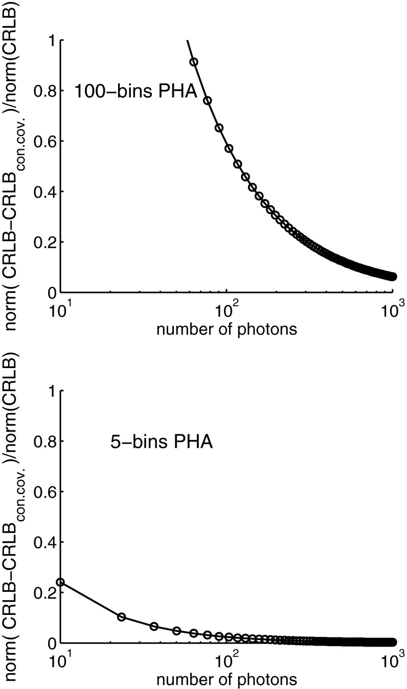
Studying the two terms, the constant covariance term includes ${\mathbf{C}}_{\mathbf{L}}^{-\mathbf{1}}$, which is roughly proportional to photon counts, while the second term, which has the product of C_L and its inverse, does not increase with photon counts. Therefore, we would expect the constant covariance term to dominate the Fisher matrix and the CRLB as photon count increases. The Appendix shows simulations that verify this conjecture. The second term is negligible for photon counts greater than approximately 100 for 5 PHA bins and 1000 with 100 PHA bins.

Using the constant covariance approximation to gain insight into the additional variance, suppose we partition the basis function matrix M into its columns and, for simplified notation, consider the three function case

We can then write the constant covariance term of the Fisher matrix using partitioned matrix notation as

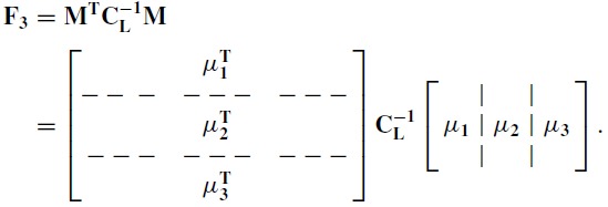(16)

Comparing Eq. 16 with the partitioning of the Fisher matrix in Eq. 6 for the dimension 3 case,

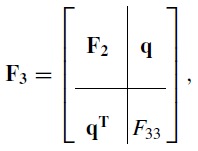the vector q is

$$\mathbf{q}=\left[\begin{array}{c}{\mu }_{\mathbf{1}}^{\mathbf{T}}{\mathbf{C}}_{\mathbf{L}}^{-\mathbf{1}}{\mu }_{\mathbf{3}}\\ {\mu }_{\mathbf{2}}^{\mathbf{T}}{\mathbf{C}}_{\mathbf{L}}^{-\mathbf{1}}{\mu }_{\mathbf{3}}\end{array}\right].$$ (17)

From the discussion in Sec. 2D, the additional CRLB covariance depends on R_2q. Since the two-dimension CRLB, R₂, is positive definite, the additional covariance is proportional to q.

We can interpret the elements of q as the weighted inner products of the third basis vector with the first two basis vectors using the inverse measurement covariance matrix as the weighting function. With a photon counting PHA detector, the inverse of the variance is equal to the expected value of the counts in each measurement bin so the weighting function is the x-ray spectrum. The components of q and therefore the additional covariance will be zero only if the third basis function μ₃ is orthogonal to μ₁ and to μ₂ using the weighted inner product.

Simulations of increase in CRLB

Simulations were used to quantify the increase in covariance under different circumstances. A 120 kilovolt (kV) x-ray tube spectrum in 1 keV bins was generated using the TASMIP algorithm.²⁵ The number of photons per measurement was adjusted by multiplying by a constant so the spectrum integral was equal to the desired number for each trial. The expected numbers of transmitted photons for each pixel and PHA energy bin were computed from the source spectrum, the thicknesses of each of the materials in the object, and their attenuation coefficients as a function of energy using exponential transmission with good geometry so scatter was negligible. The attenuation coefficients of the object materials were computed from the Hubbell-Seltzer²⁶ database using elemental compositions from ICRU Report 44.²⁷ The Hubbell-Seltzer attenuation coefficient values were interpolated using piecewise continuous Hermite polynomials in log attenuation coefficient, log photon energy. Random statistically independent Poisson distributed data with the expected counts for each pixel and energy bin were then computed. The independent Poisson distribution is a valid statistical model if the detector is quantum noise limited and pulse pileup is negligible.^{28, 29} The quantum-noise limited assumption means that electronic noise and other system imperfections are much smaller than photon counting noise.

The object materials were cortical bone, soft and adipose tissue, and a contrast agent with composition one percent iodine by weight in water. The CRLB was computed using the inverse of the full Fisher matrix in Eq. 13 using Eq. 14 to compute the derivatives in the second term. The data were processed with the A-space method with a basis set consisting of the attenuation coefficients of bone and soft tissue for the two function case and adding either the attenuation coefficient of adipose tissue or the contrast agent as the third basis function.

Additional variance as a function of photon number and third basis function

The CRLB variance of the bone and soft tissue A-vectors was computed using a two or three function basis set as a function of the total number of photons. The results were repeated with the adipose tissue or the iodine contrast agent as the third basis material. The results were plotted on log-log scales to show the functional dependence.

Effect of object thickness

As the object thickness increases, beam hardening will selectively attenuate the lower energy photons thereby increasing the average energy and reducing the spectral bandwidth and therefore increasing the noise variance. This was studied by filtering the 120 kV spectrum with a soft tissue object of varying thickness. The transmitted spectrum was used with Eq. 12 to compute the measurement covariance and then with Eq. 13 to compute the CRLB for each thickness. From the CRLB, the variance of the bone and soft tissue components was plotted as a function of the thickness. The number of transmitted photons for each thickness was kept constant to allow us to separate the effect of the spectrum change and the number of photons. This was done by normalizing the transmitted spectrum by dividing its integral and then multiplying by the fixed number of photons, 10⁷. This constant was chosen to be equal to the largest value used in the image simulations.

Effect of detector energy resolution

The effect of the detector energy resolution was simulated by computing the additional variance for PHA detectors with different number of energy bins. This requires a computation of the M matrix and the covariance for the limited resolution detectors. For this computation, the energy response for each energy bin was assumed to be a rectangle function equal to one inside the energy bin and zero otherwise. The elements of M are the effective values of the basis functions for the spectrum of each bin as given by Eq. 11 and the measurement covariance is given by Eq. 12 with the N_k computed with Eq. 3.

Simulated images from energy selective x-ray data

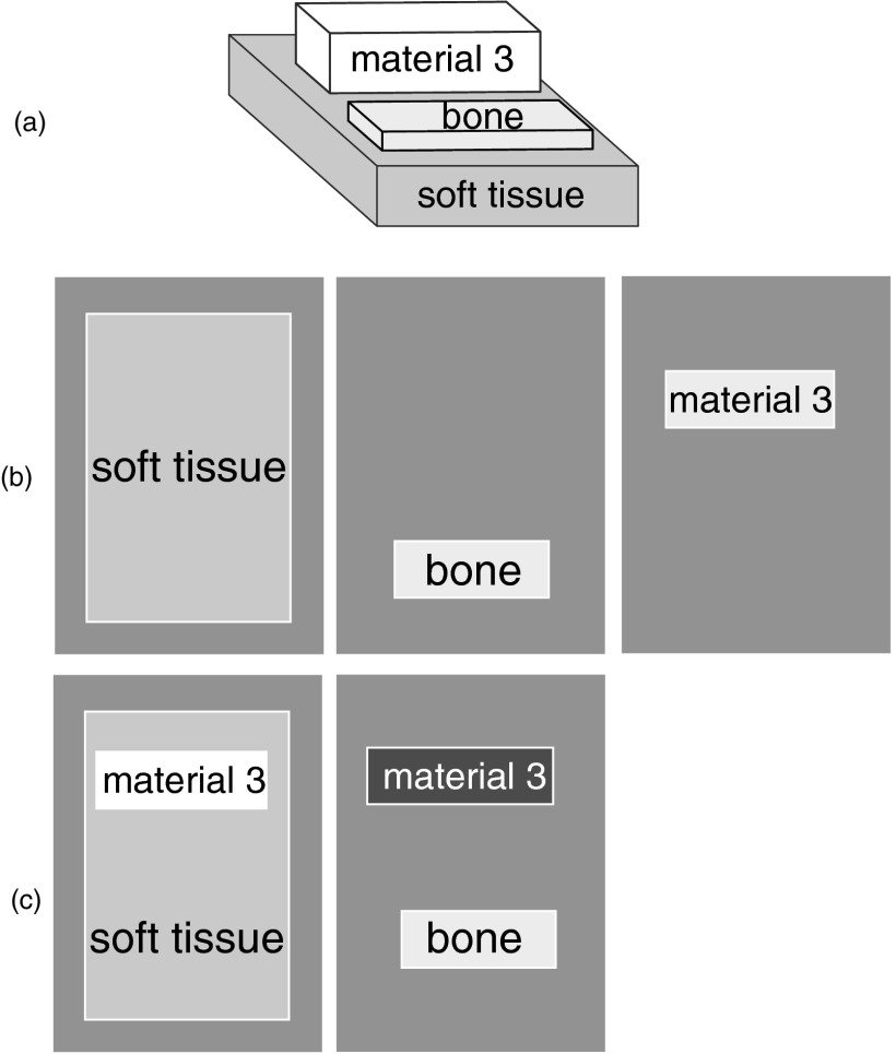
The theoretical results derived in Secs. 2A, 2B, 2C, 2D were illustrated with simulated x-ray images of the object in Fig. 1. The object, shown in perspective in Fig. 1a, is composed of blocks of three materials: soft tissue, cortical bone, and a third material that can be either adipose tissue or the iodine contrast agent. The source spectrum, object attenuation coefficients and PHA detector are as described in Sec. 2E. The object dimensions shown in the figure are not intended to model a typical medical application but to illustrate the effects of dimensionality on noise. The photons transmitted through the object are measured with a PHA detector in each pixel. Poisson distributed random samples of the transmitted spectrum for each pixel and PHA energy bin were generated and logarithms of the data divided by the number of photons incident on the object in each bin were computed. The data in separate energy bins and pixels are statistically independent.

Figure 1.

The object for the images with noise simulation. The object is composed of blocks of tissue shown in perspective view in part (a). The thicknesses of the blocks was 1 cm for adipose tissue and 0.1 cm for the bone or the iodine contrast material. The soft tissue thickness for the noise vs dimensionality simulations was 1 cm but was varied from 1 to 30 cm for the noise vs object thickness simulation. Part (b) shows the A-vector components as they might be imaged by a three dimension system with adipose tissue as the third basis material. Part (c) shows the components for a two dimension system. In this case, the adipose tissue appears as a positive amount of soft tissue and a negative amount of bone.

The random PHA data vectors L in each pixel were processed first with three and then with two function basis sets. Each bin is a separate effective measurement so there are many more measurements than dimensions. A linear maximum likelihood estimator assuming constant covariance was used. With the multivariate normal noise distribution, this estimator is²⁴

$${\widehat{\mathbf{A}}}_{MLE}=\left[{\left({\mathbf{M}}^T{\mathbf{C}}_L^{-1}\mathbf{M}\right)}^{-1}{\mathbf{M}}^{\mathbf{T}}{\mathbf{C}}_{\mathbf{L}}^{-\mathbf{1}}\right]\mathbf{L}.$$ (18)

In Eq. 18, the term in brackets is a constant matrix since the measurement covariance C_L is assumed to be constant. This allows the estimated A-vector at each pixel to be computed by a matrix multiplication. The measurement covariance was computed from the energy spectrum in the soft tissue region. Since the covariance depends on the object thickness, this can lead to errors and A-vector noise covariance greater than the CRLB. However, the simulated results show that the linear estimator gave good performance with the relatively thin object used.

The estimators for two and three dimensions were computed with Eq. 18 using M matrices with two or three columns equal to the attenuation coefficients of the basis materials evaluated at the PHA energy bin boundaries. The same measurement data L were used with both estimators so the noise in the results is directly inter-comparable.

The variance of samples of the A-vector image data in the soft tissue region that does not overlap the blocks of other materials was computed. This was plotted as a function of the number of photons. The CRLB was also computed using Eq. 13 from the known spectrum and plotted for comparison with the image noise.

Low noise conventional images from energy selective data

As shown in my previous paper,¹³ we can use energy selective data to produce images with data comparable to conventional photon counts or integrated energy but with larger SNR. To illustrate this, the random measurement data were used to make two images. One was an image of the total number of photons in each pixel. The second used the two dimension A-vectors. The vectors at every pixel were transformed by multiplying by a “whitening” matrix¹³ so their components have equal variance and are uncorrelated. Then a generalized projection was computed by forming an inner product of the whitened A-vectors with a unit vector with an angle chosen to optimize the difference between the bone-region and the “air” data outside the object.

RESULTS

Additional variance as a function of dimensionality and photon number

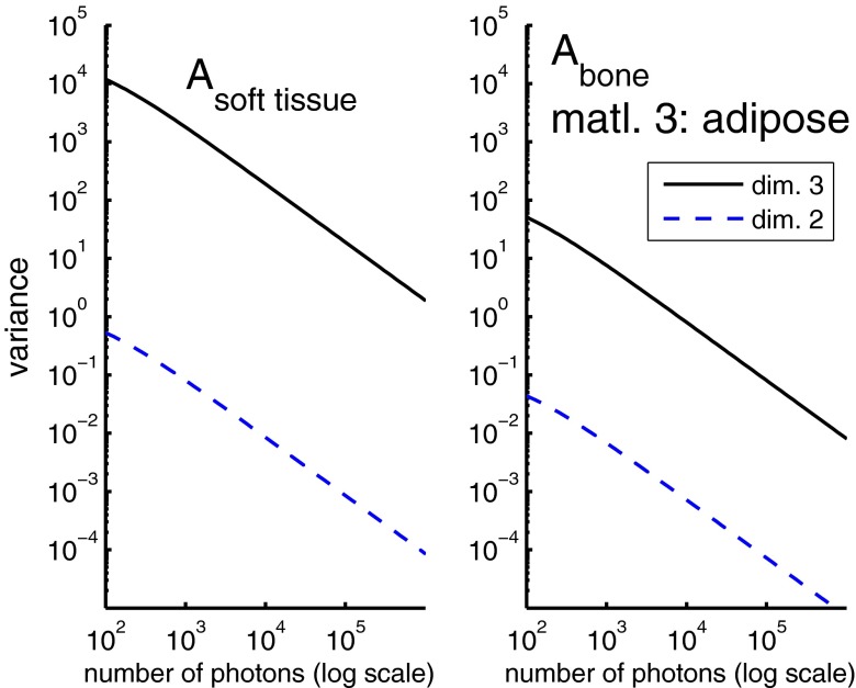
Figure 2 shows the variance of the first two A-vector components with two and three dimension processing as a function of the total number of photons per pixel. The left panel shows the variance of the soft tissue component while the right panel shows the variance of the bone component.

Figure 2.

The variance for the soft tissue and bone A-vector components as a function of photon number with two and three dimension processing. The third basis function was the attenuation coefficient of adipose tissue. The left panel shows the variance of ${\mathrm{A}}_{\mathrm{soft}\mathrm{tissue}}$ and the right panel is the variance of ${\mathrm{A}}_{\mathrm{bone}}$.

The x and y scales are logarithmic so the variance is inversely proportional to the photon number in all cases. The variance with three dimensions is much larger than the variance with two dimensions. At the same photon number, the three dimension bone component variance is 1.4 × 10³ larger than the two dimension value. The soft tissue component variance increase is 2.7 × 10⁴.

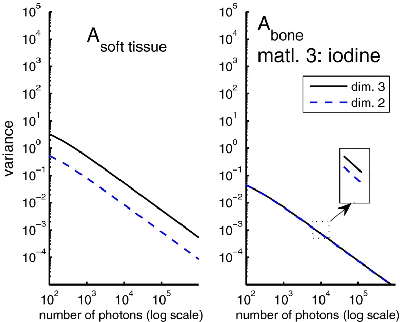
Figure 3 shows the variance of the first two A-vector components when the third basis function is the attenuation coefficient of a mixture of iodine and water. In this case, the variance of both components only increases slightly from two to three basis functions. The bone component variances are so close that they are hard to see in the plot but the zoom inset shows that there is indeed a small increase from two to three dimensions as expected. The variance increases from two to three dimensions by factors of 1.03 and 7.4 for the bone and soft tissue components, respectively.

Figure 3.

Variance as a function of photon number when the third basis function is the attenuation coefficient of one percent (by weight) iodine in water. The increase in variance of the bone component from two to three dimensions is small but positive as shown by the zoom inset.

Additional variance vs object thickness

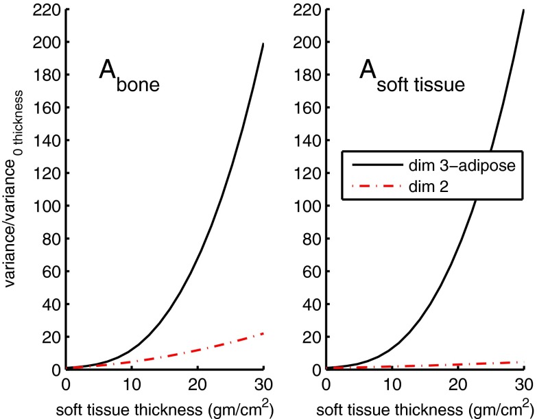
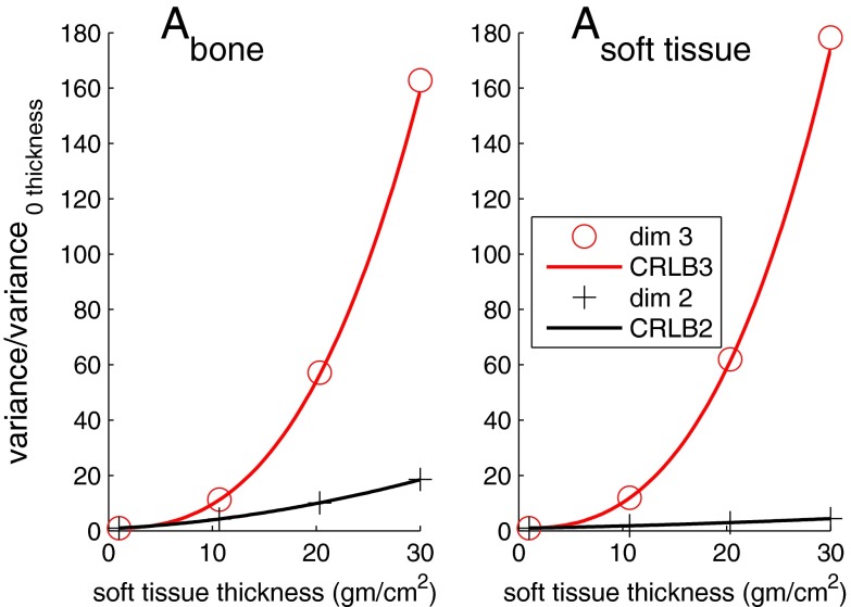
Figure 4 shows the effect of increasing the object thickness on the variance. In the computation of the data, the total number of transmitted photons was kept fixed at each object thickness by increasing the total number of photons in the incident spectrum but otherwise not changing its shape. The object was assumed to be composed of soft tissue. Other body materials such as bone will give curves with different shapes but will also harden the spectrum and increase the variance. The ratio of the variance for each thickness divided by the variance with zero thickness is plotted so the results are independent of the transmitted photon number. The increase from 1 to 30 cm was approximately a factor of 200 for the bone component and 220 for the soft tissue component.

Figure 4.

Additional variance vs object thickness. The photon number is constant for each thickness so that the increase in variance is due to the effect of beam hardening. Plotted is the ratio of the variance at each thickness to the variance with zero thickness. The third basis function is the attenuation coefficient of adipose tissue.

Additional variance vs detector energy resolution

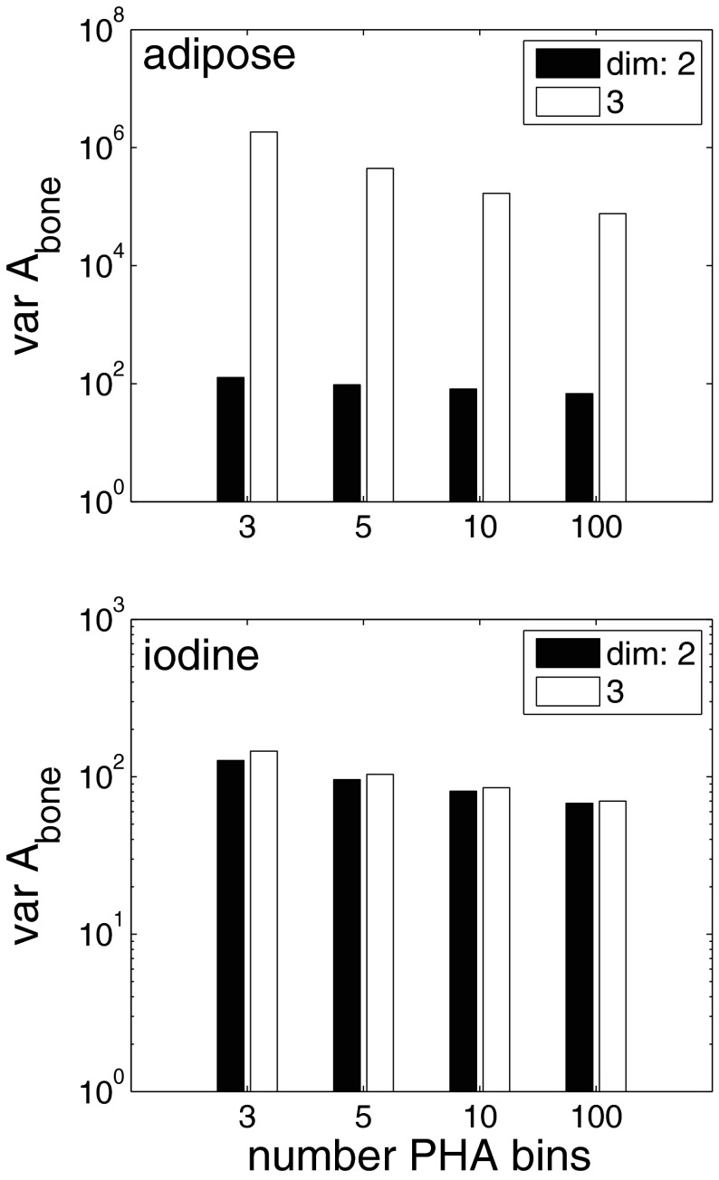
The effect of the detector energy resolution is shown in Fig. 5. The figure plots the variance of the bone component for PHA with 3, 5, 10, and 100 energy bins. For the 3, 5, and 10 bin cases, the bins were contiguous with widths adjusted to give the same number of photons. With the 100 bin detector, the bins were equally spaced across the spectrum.

Figure 5.

Additional variance vs detector energy resolution. Plotted is the A_bone variance with two and three basis functions for 3 to 100 bins PHA. In the top panel, the third basis function is the attenuation coefficient of adipose tissue while in the bottom panel it is the attenuation coefficient of one percent iodine in water. The vertical scale is logarithmic.

In the top panel, the additional basis function was the attenuation coefficient of adipose tissue and in the bottom panel it was the attenuation coefficient of the iodine and water mixture. With three dimension processing and adipose tissue as the third basis material, the bone component variance increases markedly, a factor of 25 from 100 bins to the 3 bin value. The increase with two dimension processing is much less, a factor of approximately two. The increase is variance with the contrast agent as the third basis material is smaller and about the same with either three or two dimension processing, a factor of two for the bone and soft tissue A-vector components.

Simulated images

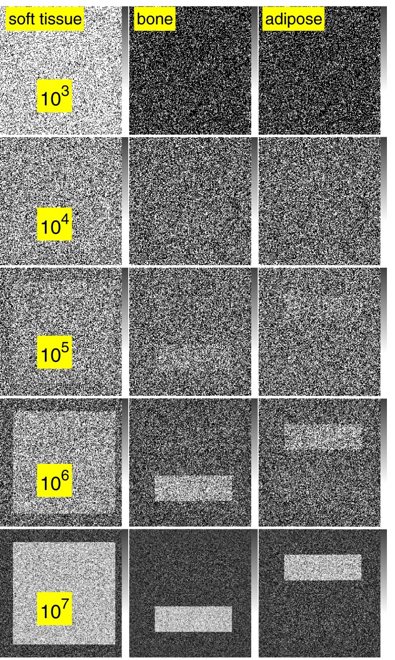
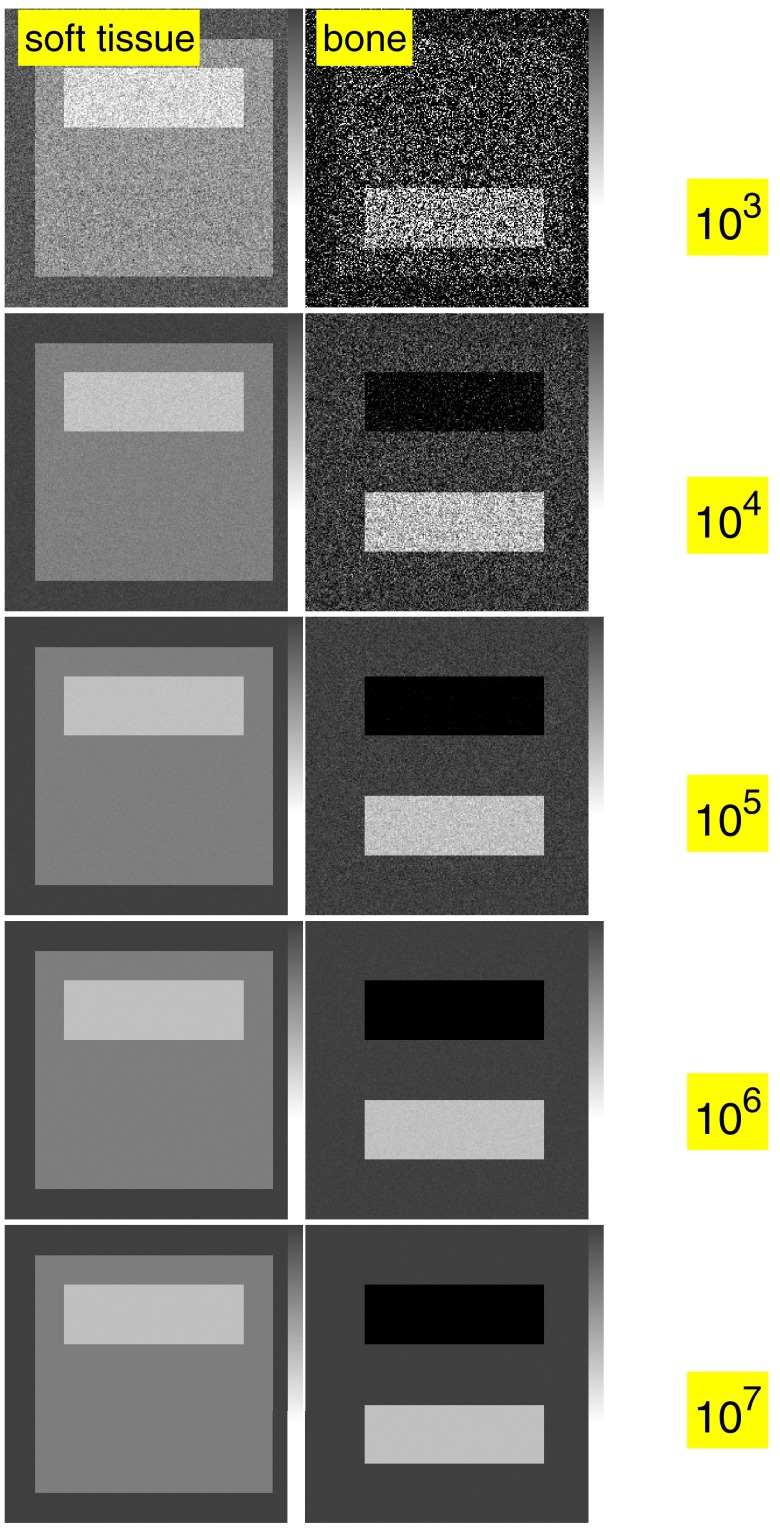
Simulated images with three dimension processing are shown in Fig. 6 and with two dimension processing in Fig. 7.

Figure 6.

Simulated images with three dimension processing when the third basis function is the attenuation coefficient of adipose tissue. A-space processing is used with 100 energy bin PHA data to compute the effective line integrals with a basis set consisting of the attenuation coefficients of soft tissue, adipose tissue, and cortical bone. The A-vector components are shown in the three columns. For each row, the spectra are multiplied by a constant so the expected number of photons per pixel increases from 10³ in the top row to 10⁷ in the bottom row. Note the gray bar at the right of each image with a range from 0 to 2.5 cm.

Figure 7.

The noisy data in Fig. 6 are processed using a two dimension basis set. The noise is much less but the adipose tissue is not imaged separately and it appears as a positive amount of soft tissue and a negative amount of bone.

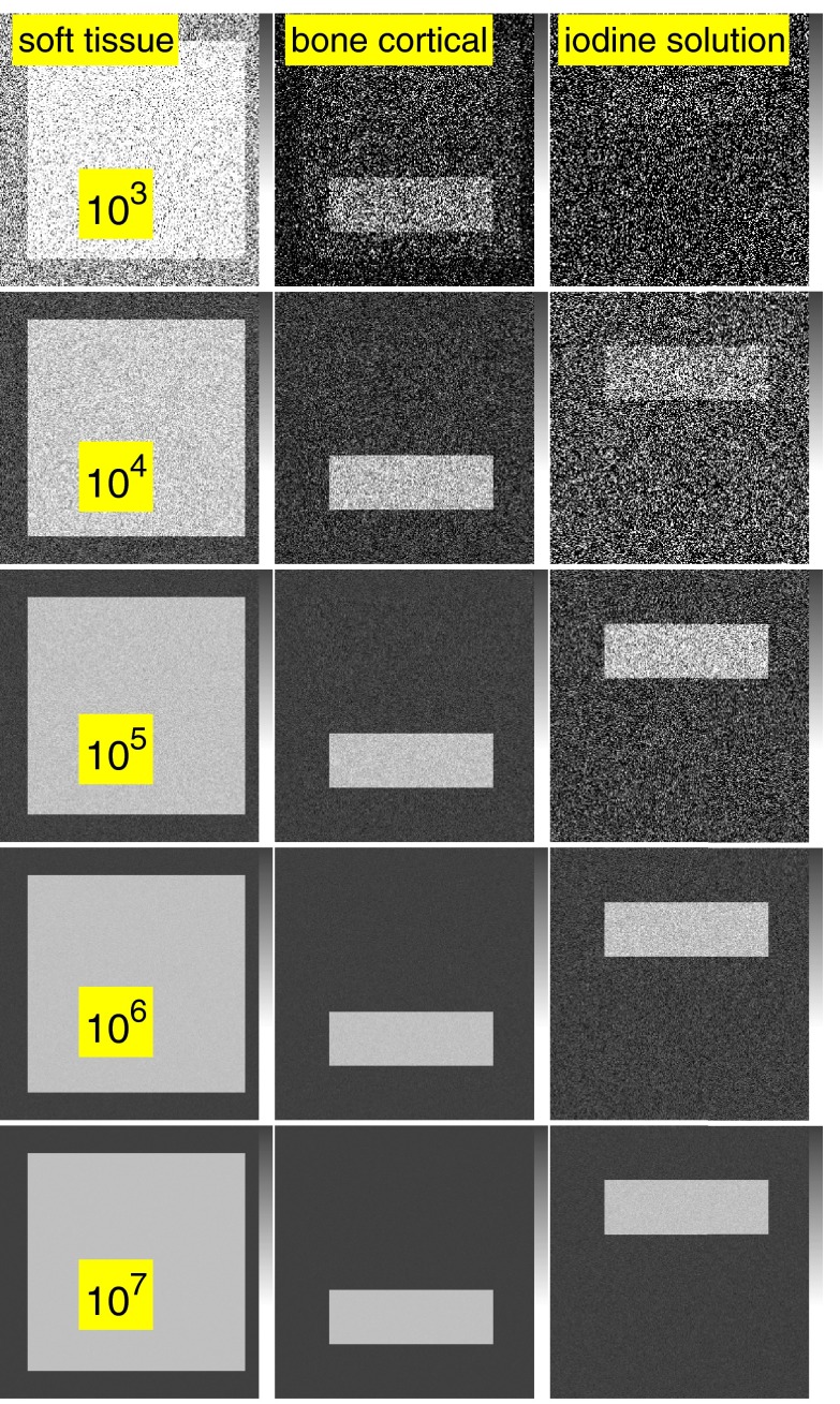
The effect of the third basis function is shown in Fig. 8. In this figure, the third basis function is the attenuation coefficient of one percent fraction by weight of iodine in water. The number of photons for each row is the same as in Figs. 67.

Figure 8.

The PHA data are processed using a basis set consisting of the attenuation coefficients of soft tissue, cortical bone, and one percent iodine in water solution. Compare the noise in these images with Fig. 6, which uses the attenuation coefficient of adipose tissue as the third basis function.

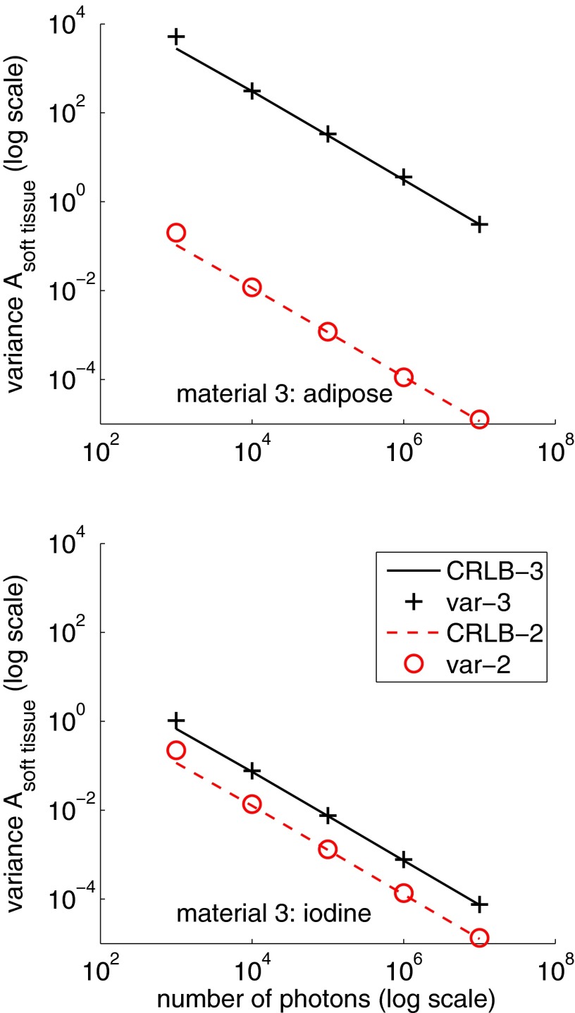
The variance of the A-vector data in the soft tissue region of the images with noise as a function of the number of photons per pixel is plotted in Fig. 9. The CRLB computed using the spectrum in the soft tissue region is plotted as the solid lines for each case.

Figure 9.

A-vector variance in the soft tissue region of the images. In the top graph, the third basis function is the attenuation coefficient of adipose tissue. In the bottom graph, it is the attenuation coefficient of iodine in water. The crosses and circles are the image sample variance and the solid lines are the CRLB. Both axis scales are logarithmic.

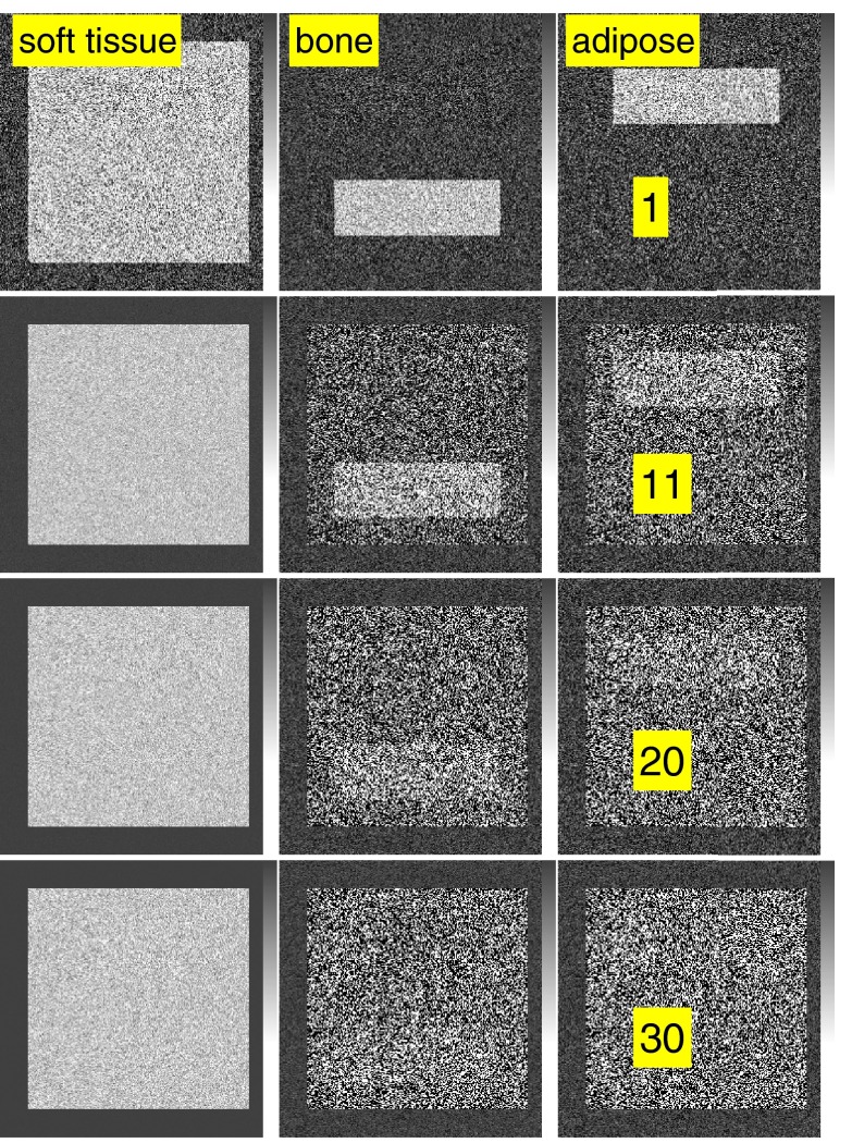
The effect of beam hardening is illustrated by the images in Fig. 10. In the figure, the thickness of the soft tissue, shown in the right column, was increased from 1 to 30 cm. The number of transmitted photons per pixel was fixed at 10⁷ by increasing the incident number of photons as the thickness increases. The image variance values are plotted in Fig. 11 as a function of the thickness. The CRLB values computed from the spectrum in the soft tissue region are also plotted as the solid lines.

Figure 10.

Images illustrating the effects of beam hardening on basis image noise. Each row shows the basis images for different soft tissue slab thicknesses from 1 to 30 cm. The thicknesses are labeled in the right column. See Fig. 1 for a description of the phantom. The number of transmitted photons per pixel was fixed at 10⁷ for all four cases by increasing the number of incident photons as the thickness increases.

Figure 11.

Noise variance in the images in Fig. 10 as a function of soft tissue slab thickness. The variance of the image data within the soft tissue excluding the regions where bone and adipose tissue blocks overlap is used. The image data sample variances for three dimension processing are the circles while for two dimension processing they are the cross symbols. The CRLB for each type of processing is plotted as the solid lines.

As the soft tissue thickness increases, the large difference between the air region and the object causes errors with the linear maximum likelihood estimator so the soft tissue object appears in the bone and adipose tissue basis images. However, within the soft tissue region the contrast if the bone and adipose tissue blocks is lower and the linear estimator noise variance is equal to the CRLB.

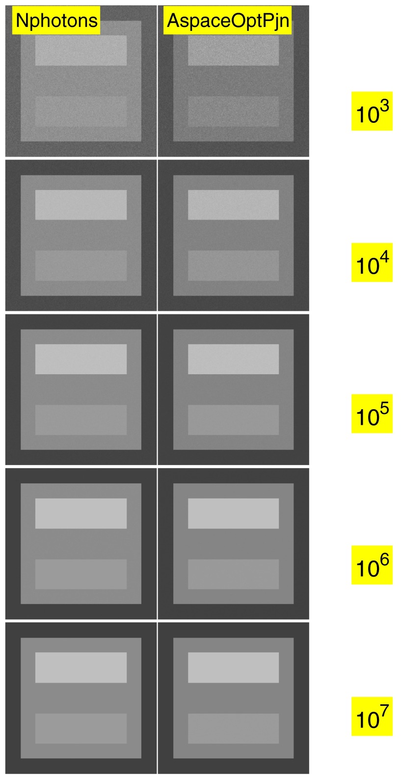
Computing low noise images with energy selective data is illustrated in Fig. 12. In the figure, images with data equal to the number of photon in each pixel are in the left column and the optimal generalized projection images computed from the A-vector data as discussed in Sec. 2G are in the right column. The number of photons per pixel increases from the top to the bottom row as labeled on the images. The photon numbers were the same as in Figs. 67 so the noise in the images can be directly compared.

Figure 12.

Low noise images from energy selective data. The image data in the left column are the total number of photons per pixel. The data in the right column are computed from the two-dimension A-vectors by transforming so the variances of the components are equal and uncorrelated. Then a dot product is computed of the transformed A-vector in each pixel with a unit vector at an angle selected to maximize the bone contrast.

DISCUSSION

The images in Sec. 3D illustrate the trade-off between dimensionality and noise. Figure 6 shows that a three dimension basis set has more information since we can image bone, soft tissue, and adipose tissue separately while with the two dimension set in Fig. 7 the adipose tissue appears as a positive amount of soft tissue and a negative amount of bone. However, for comparable numbers of transmitted photons per pixel, the three dimension images have much larger noise variance than the two dimension images, 1.4 × 10³ and 2.7 × 10⁴ times larger for the bone and soft tissue components, respectively.

Figure 8 shows that the properties of the basis functions have a strong effect on the noise. In this figure, the third basis function is the attenuation coefficient of a one percent mixture of iodine in water. The number of photons for each row of this image are the same as in Fig. 6 but the noise variance is much smaller. The increase from two to three dimensions is 1.03 and 7.4 for the bone and soft tissue components in this case.

Figure 10 illustrates the effect of spectrum changes with beam hardening on the noise. The figure shows the A-vector component images as the thickness of the soft tissue block in Fig. 1 is increased from 1 to 30 cm. The number of transmitted photons is kept constant at each thickness so the increase in noise is only due to the increase in the average energy and reduction of the spectral bandwidth with beam hardening.

The detector energy resolution has a smaller but still substantial effect. Figure 5 shows that as the resolution decreases from 100 to 3 bins the three dimension bone component variance increases by a factor of 25 with adipose tissue as the third basis material. The increase for the soft tissue component is smaller, approximately two. With the iodine mixture as the third material, the increase for both components is also approximately two. With either basis material, increasing the energy resolution allows the system to extract the A-vector information with less noise for the same number of transmitted photons.

The log-log plots in Figs. 23 show that the noise variance is inversely proportional to the number of photons so reducing the variance requires proportional increases in the number of transmitted photons. Since the dose is in turn roughly proportional to the transmitted photon number, large increases in dose may be required with the soft tissue, bone, and adipose tissue basis material set depending on the acceptable noise level for a clinical application of the data. The methods described in this paper can be used by medical physicists working with clinicians to optimize parameters for a particular application and to decide whether the increased dose required to extract the higher dimension information is justified by its diagnostic value.

The simulations in this paper assume that the detectors are quantum noise limited and satisfying this requirement with high counts places stringent limits on the detector electronic noise levels and other imperfections that may be beyond the present state of the art. The increases in noise with the contrast agent as the additional basis material are much smaller so this application is more feasible with current technology.

Conventional systems that measure only the total photon energy or the total number of photons do not extract the information present in the energy spectrum. Figure 12 shows that by using the spectrum information, we can produce images with higher signal to noise ratio than images of the number of photons.

The computation of images with variance close to the CRLB requires a suitably chosen statistical estimator. An estimator that results in variance equal to the CRLB is called “efficient” and the maximum likelihood estimator used in the simulations is known to be asymptotically efficient in the limit of a large number of observations.³⁰ No general method is known to determine the actual number of observations required to give efficient performance but the image simulations show that the linear estimator described by Eq. 18 is efficient with the ranges of photon counts used.

The linear assumption was not valid over the transition from the “air” region to the object for the large soft tissue thicknesses in Fig. 10 causing errors in this region. However, general maximum likelihood estimators have been developed that are usable over large object thickness variations. Roessl and Proksa³¹ describe an iterative maximum likelihood estimator that was used by Schlomka et al.³² to make experimental images of an 8 cm phantom with photon counting detectors with PHA. Alvarez³³ describes a noniterative estimator for two dimension processing that achieves the CRLB with object thicknesses up to 30 cm.

The implementation by Schlomka et al.³² while impressive had implementation problems including long and unpredictable computation with the iterative algorithm and requiring measurements of the source spectrum and detector energy response that are difficult in clinical settings. The implementation by Alvarez³³ addressed these problems but only a two-dimensional estimator was described. Development of estimators for higher dimensions that achieve the CRLB and can be implemented in clinical systems should be addressed by future research.

The x-ray detectors used in the simulations were idealized by assuming quantum limited noise and negligible pulse pileup. The CRLB is applicable with nonidealized detectors if good models^{28, 29} of detector noise are available. These models can be used with the CRLB to determine the effects of nonideal detector performance on dimensionality, to optimize the detectors, and to develop estimators that provide efficient performance.

CONCLUSION

A method based on the Cramèr-Rao lower bound is presented to quantify the increase in noise variance with dimensionality. This method allows us to study the trade-off of the additional information with the increased dose required to extract it. The increase in noise variance from two to three dimensions will depend on the source spectrum, the object composition and thickness, the detector energy resolution, and the basis set used. Even with very high energy resolution data, the increase in variance from two to three dimensions with the soft tissue, bone, and adipose tissue basis material set, 1.4 × 10³ and 2.7 × 10⁴ for bone and soft tissue, respectively, is so large that extracting it will be difficult. With the attenuation coefficient of an iodine contrast agent as the third basis function, the increase in variance is much smaller, 1.03 and 7.4, so extracting higher dimension information in this case may be feasible as detector technology advances. The method is applicable with different types of energy selective systems and can be used by x-ray system designers for optimizing energy selective system parameters. It can also be used by medical physicists working with clinicians to optimize parameters for a particular application and to decide whether the increased dose required to extract the higher dimension information is justified by its diagnostic value.

APPENDIX: CONSTANT COVARIANCE APPROXIMATION TO THE CRLB OF ENERGY SELECTIVE SYSTEMS

The error using only the constant covariance term was calculated as the norm of the difference of the complete CRLB covariance computed using Eq. 13 and the CRLB computed using only the first term in the Fisher matrix, Eq. 15, which assumes the covariance is constant. The fractional error was computed as the norm of the difference divided by the norm of the complete CRLB,

$$\text{frac.err.}=\frac{\Vert {\mathbf{R}}_{\mathbf{A},\mathbf{CRLB}}-{\mathbf{R}}_{\mathbf{A},\mathbf{CRLB},\mathbf{con}.\mathbf{cov}}\Vert }{\Vert {\mathbf{R}}_{\mathbf{A},\mathbf{CRLB}}\Vert }.$$ (A1)

See Section 2C for a description of the formulas used to compute the terms in this equation.

Simulations were performed to compute the error with PHA detectors as a function of the photon counts and the energy resolution. A 120 kV x-ray tube spectrum was used with a basis set consisting of the attenuation coefficients of soft tissue, cortical bone, and adipose tissue. Two different PHA detectors with 100 bins or 5 bins were assumed. The 100 bins were uniformly spaced while the 5 bins were chosen to give equal number of transmitted photons in each bin. The bins in both cases were contiguous and spanned the complete spectrum.

The error shown in Fig. 13 decreases with either detector as the number of photons increases. The error is negligible for photon numbers greater than approximately 100 for the 5 bin detector and 1000 for the 100 bin detector. Evidently the number of photons per bin has a significant effect on the error so more photons are required with larger number of bins.

Figure 13.

Error using the constant covariance CRLB as a function of photon counts. The top panel shows the error with 100 PHA bins while the bottom panel is for 5 bins. The error decreases as the number of photons increases. Note the logarithmic horizontal axis scale.

References

- Alvarez R. E. and Macovski A., “Energy-selective reconstructions in x-ray computerized tomography,” Phys. Med. Biol. 21, 733–44 (1976). 10.1088/0031-9155/21/5/002 [DOI] [PubMed] [Google Scholar]
- Iwanczyk J. S., Nygard E., Meirav O., Arenson J., Barber W. C., Hartsough N. E., Malakhov N., and Wessel J. C., “Photon counting energy dispersive detector arrays for x-ray imaging,” IEEE Trans. Nuc. Sci. 56(3), 535–542 (2009). 10.1109/TNS.2009.2013709 [DOI] [PMC free article] [PubMed] [Google Scholar]
- Aslund M., Fredenberg E., Telman M., and Danielsson M., “Detectors for the future of x-ray imaging,” Radiat. Prot. Dosim. 139, 327–333 (2010). 10.1093/rpd/ncq074 [DOI] [PubMed] [Google Scholar]
- Evans R. D., The Atomic Nucleus (McGraw-Hill, New York, 1955). [Google Scholar]
- Alvarez R. E., “Energy dependent information in x-ray imaging—Part 1: The vector space description,” Stanford University Information Systems Laboratory (1982) (unpublished).
- Lehmann L. A. and Alvarez R. E., Energy Selective Radiography: A Review (Plenum Press, New York, 1986), pp. 145–187. [Google Scholar]
- Van Trees H. L., Detection, Estimation, and Modulation Theory. Part I: Detection, Estimation, and Linear Modulation Theory (John Wiley & Sons Inc., New York, 2001). [Google Scholar]
- Kay S. M., Fundamentals of Statistical Signal Processing. Volume I: Estimation Theory (Prentice Hall PTR, Upper Saddle River, NJ, 1993). [Google Scholar]
- van den Bos A., Parameter Estimation for Scientists and Engineers (Wiley-Interscience, Hoboken, NJ, 2007). [Google Scholar]
- Kay S. M., Fundamentals of Statistical Signal Processing. Volume I: Estimation Theory (Prentice Hall PTR, Upper Saddle River, NJ, 1993), Chap. 3. [Google Scholar]
- van den Bos A., Parameter Estimation for Scientists and Engineers (Wiley-Interscience, Hoboken, NJ, 2007), Sec. 4.6.5. [Google Scholar]
- Tapiovaara M. J. and Wagner R., “SNR and DQE analysis of broad spectrum x-ray imaging,” Phys. Med. Biol. 30, 519–529 (1985). 10.1088/0031-9155/30/6/002 [DOI] [Google Scholar]
- Alvarez R. E., “Near optimal energy selective x-ray imaging system performance with simple detectors,” Med. Phys. 37, 822–841 (2010). 10.1118/1.3284538 [DOI] [PMC free article] [PubMed] [Google Scholar]
- Weaver J. B. and Huddleston A. L., “Attenuation coefficients of body tissues using principal-components analysis,” Med. Phys. 12, 40–45 (1985). 10.1118/1.595759 [DOI] [PubMed] [Google Scholar]
- Gingold E. L. and Hasegawa B. H., “Systematic bias in basis material decomposition applied to quantitative dual-energy x-ray imaging,” Med. Phys. 19, 25–33 (1992). 10.1118/1.596889 [DOI] [PubMed] [Google Scholar]
- Williamson J. F., Li S., Devic S., Whiting B. R., and Lerma F. A., “On two-parameter models of photon cross sections: application to dual-energy CT imaging,” Med. Phys. 33, 4115–4129 (2006). 10.1118/1.2349688 [DOI] [PubMed] [Google Scholar]
- Bornefalk H., “XCOM intrinsic dimensionality for low-z elements at diagnostic energies,” Med. Phys. 39, 654–657 (2012). 10.1118/1.3675399 [DOI] [PubMed] [Google Scholar]
- Stewart G. W., Introduction to Matrix Computations (Academic Press, New York, 1973). [Google Scholar]
- Roth E., “Multiple-energy selective contrast material imaging,” Ph.D. dissertation, Stanford University, 1984. [Google Scholar]
- Jolliffe I. T., Principal Component Analysis (Springer-Verlag, New York, 2002), Sec. 3.5. [Google Scholar]
- Alvarez R. E. and Seppi E. J., “A comparison of noise and dose in conventional and energy selective computed tomography,” IEEE Trans. Nuc. Sci. NS-26, 2853–2856 (1979). 10.1109/TNS.1979.4330549 [DOI] [Google Scholar]
- Harville D. A., Matrix Algebra from a Statistician's Perspective (Springer, New York, 2008), Corollary 14.2.3. [Google Scholar]
- Kay S. M., Fundamentals of Statistical Signal Processing. Volume I: Estimation Theory (Prentice Hall PTR, Upper Saddle River, NJ, 1993), Sec. 3.9. [Google Scholar]
- Kay S. M., Fundamentals of Statistical Signal Processing. Volume I: Estimation Theory (Prentice Hall PTR, Upper Saddle River, NJ, 1993), Sec. 4.5. [Google Scholar]
- Boone J. M. and Seibert J. A., “An accurate method for computer-generating tungsten anode x-ray spectra from 30 to 140 kV,” Med. Phys. 24, 1661–1670 (1997). 10.1118/1.597953 [DOI] [PubMed] [Google Scholar]
- Hubbell J. H. and Seltzer S. M., “Tables of x-ray mass attenuation coefficients and mass energy-absorption coefficients,” National Institute of Standards and Technology (available URL: http://physics.nist.gov/PhysRefData/XrayMassCoef/cover.html).
- ICRU, “Report 44: Tissue substitutes in radiation dosimetry and measurement,” International Commission on Radiological Units and Measurements (available URL: http://www.icru.org).
- Taguchi K., Zhang M., Frey E. C., Wang X., Iwanczyk J. S., Nygard E., Hartsough N. E., Tsui B. M. W., and Barber W. C., “Modeling the performance of a photon counting x-ray detector for CT: Energy response and pulse pileup effects,” Med. Phys. 38, 1089–1102 (2011). 10.1118/1.3539602 [DOI] [PMC free article] [PubMed] [Google Scholar]
- Wang A. S., Harrison D., Lobastov V., and Tkaczyk J. E., “Pulse pileup statistics for energy discriminating photon counting x-ray detectors,” Med. Phys. 38, 4265–4275 (2011). 10.1118/1.3592932 [DOI] [PubMed] [Google Scholar]
- van den Bos A., Parameter Estimation for Scientists and Engineers (Wiley-Interscience, Hoboken, NJ, 2007), Sec. 5.3. [Google Scholar]
- Roessl E. and Proksa R., “K-edge imaging in x-ray computed tomography using multi-bin photon counting detectors,” Phys. Med. Biol. 52, 4679–4696 (2007). 10.1088/0031-9155/52/15/020 [DOI] [PubMed] [Google Scholar]
- Schlomka J. P., Roessl E., Dorscheid R., Dill S., Martens G., Istel T., Bäumer C., Herrmann C., Steadman R., Zeitler G., Livne A., and Proksa R., “Experimental feasibility of multi-energy photon-counting K-edge imaging in pre-clinical computed tomography,” Phys. Med. Biol. 53, 4031–4047 (2008). 10.1088/0031-9155/53/15/002 [DOI] [PubMed] [Google Scholar]
- Alvarez R. E., “Estimator for photon counting energy selective x-ray imaging with multi-bin pulse height analysis,” Med. Phys. 38, 2324–2334 (2011). 10.1118/1.3570658 [DOI] [PMC free article] [PubMed] [Google Scholar]