A Selective Review of Group Selection in High-Dimensional Models

Abstract

Grouping structures arise naturally in many statistical modeling problems. Several methods have been proposed for variable selection that respect grouping structure in variables. Examples include the group LASSO and several concave group selection methods. In this article, we give a selective review of group selection concerning methodological developments, theoretical properties and computational algorithms. We pay particular attention to group selection methods involving concave penalties. We address both group selection and bi-level selection methods. We describe several applications of these methods in nonparametric additive models, semiparametric regression, seemingly unrelated regressions, genomic data analysis and genome wide association studies. We also highlight some issues that require further study.

1. INTRODUCTION

Consider a linear regression model with p predictors. Suppose the predictors can be naturally divided into J nonoverlapping groups, and the model is written as

$$\mathbf{y}=\sum _{j=1}^J{X}_j{\mathit{\beta }}_j+\mathit{\epsilon },$$ (1.1)

where y is an n×1 vector of response variables, X_j is the n × d_j design matrix of the d_j predictors in the jth group, β_j = (β_j1, …, β_jdj)′ ∈ ℝ^d_j is the d_j × 1 vector of regression coefficients of the jth group and ε is the error vector. Without loss of generality, we take both the predictors and response to be centered around the mean. It is desirable to treat each group of variables as a unit and take advantage of the grouping structure present in these models when estimating regression coefficients and selecting important variables.

Many authors have considered the problem of group selection in various statistical modeling problems. Bakin (1999) proposed the group LASSO and a computational algorithm. This method and related group selection methods and algorithms were further developed by Yuan and Lin (2006). The group LASSO uses an ℓ₂ norm of the coefficients associated with a group of variables in the penalty function and is a natural extension of the LASSO (Tibshirani, 1996). Antoniadis and Fan (2001) studied a class of block-wise shrinkage approaches for regularized wavelet estimation in nonparametric regression problems. They discussed several ways to shrink wavelet coefficients in their natural blocks, which include the blockwise hard- and soft-threshold rules. Meier, van de Geer and Bühlmann (2008) studied the group LASSO for logistic regression. Zhao, Rocha and Yu (2009) proposed a quite general composite absolute penalty for group selection, which includes the group LASSO as a special case. Huang, Ma, Xie and Zhang (2009) considered the problem of simultaneous group and individual variable selection, or bi-level selection, and proposed a group bridge method. Breheny and Huang (2009) proposed a general framework for bi-level selection in generalized linear models and derived a local coordinate descent algorithm.

Grouping structures can arise for many reasons, and give rise to quite different modeling goals. Common examples include the representation of multilevel categorical covariates in a regression model by a group of indicator variables, and the representation of the effect of a continuous variable by a set of basis functions. Grouping can also be introduced into a model in the hopes of taking advantage of prior knowledge that is scientifically meaningful. For example, in gene expression analysis, genes belonging to the same biological pathway can be considered a group. In genetic association studies, genetic markers from the same gene can be considered a group. It is desirable to take into account the grouping structure in the analysis of such data.

Depending on the situation, the individual variables in the groups may or may not be meaningful scientifically. If they are not, we are typically not interested in selecting individual variables; our interest is entirely in group selection. However, if individual variables are meaningful, then we are usually interested in selecting important variables as well as important groups; we refer to this as bi-level selection. For example, if we represent a continuous factor by a set of basis functions, the individual variables are an artificial construct, and selecting the important members of the group is typically not of interest. In the gene expression and genetic marker examples, however, selection of individual genes/markers is just as important as selecting important groups. In other examples, such as a group of indicator functions for a categorical variable, whether we are interested in selecting individual members depends on the context of the study.

We address both group selection and bi-level selection in this review. The distinction between these two goals is crucial for several reasons. Not only are different statistical methods used for each type of problem, but as we will see, the predictors in a group can be made orthonormal in settings where bi-level selection is not a concern. This has a number of ramifications for deriving theoretical results and developing algorithms to fit these models.

We give a selective review of group selection concerning methodological developments, theoretical properties and computational algorithms. We describe several important applications of group selection and bi-level selection in nonparametric additive models, semiparametric regression, seemingly unrelated regressions, genomic data analysis and genome wide association studies. We also highlight some issues that require further study. For the purposes of simplicity, we focus on penalized versions of least squares regression in this review. Many authors have extended these models to other loss functions, in particular those of generalized linear models. We attempt to point out these efforts when relevant.

2. GROUP SELECTION METHODS

2.1 Group LASSO

For a column vector v ∈ ℝ^d with d ≥ 1 and a positive definite matrix R, denote ||v||₂ = (v′v)^1/2 and ||v||_R = (v′Rv)^1/2. Let $\mathit{\beta }={({\mathit{\beta }}_1^{\prime },\dots ,{\mathit{\beta }}_J^{\prime })}^{\prime }$, where β_j ∈ ℝ^d_j. The group LASSO solution β(λ) is defined as a minimizer of

$$\frac{1}{2n}{\Vert \mathbf{y}-\sum _{j=1}^J{X}_j{\mathit{\beta }}_j\Vert }_2^2+\lambda \sum _{j=1}^J{c}_j{\Vert {\mathit{\beta }}_j\Vert }_{R_j},$$ (2.1)

where λ ≥ 0 is the penalty parameter and R_j’s are d_j ×d_j positive definite matrices. Here the c_j’s in the penalty are used to adjust for the group sizes. A reasonable choice is $c_j=\sqrt{d_j}$. Because (2.1) is convex, any local minimizer of (2.1) is also a global minimizer and is characterized by the Karush–Kuhn–Tucker conditions as given in Yuan and Lin (2006). It is possible, however, for multiple solutions to exist, as (2.1) may not be strictly convex in situations where the ordinary least squares estimator is not uniquely defined.

An important question in the definition of group LASSO is the choice of R_j. For orthonormal X_j with $X_j^{\prime }{X}_j/n=I_{d_j}$, j = 1, …, J, Yuan and Lin (2006) suggested taking R_j = I_dj. However, using R_j = I_dj may not be appropriate, since the scales of the predictors may not be the same. In general, a reasonable choice of R_j is to take the Gram matrix based on X_j, that is, $R_j=X_j^{\prime }{X}_j/n$, so that the penalty is proportional to ||X_jβ_j||₂. This is equivalent to performing standardization at the group level, which can be seen as follows. Write $R_j=U_j^{\prime }{U}_j$ for a d_j × d_j upper triangular matrix U_j via Cholesky decomposition. Let ${\stackrel{\sim }{X}}_j=X_j{U}_j^{-1}$ and b_j = U_jβ_j. Criterion (2.1) becomes

$$\frac{1}{2n}{\Vert \mathbf{y}-\sum _{j=1}^J{\stackrel{\sim }{X}}_j{\mathbf{b}}_j\Vert }_2^2+\lambda \sum _{j=1}^J{c}_j{\Vert {\mathbf{b}}_j\Vert }_2.$$ (2.2)

The solution to the original problem (2.1) can be obtained by using the transformation ${\mathit{\beta }}_j=U_j^{-1}{\mathbf{b}}_j$. By the definition of U_j, we have $n^{-1}{\stackrel{\sim }{X}}_j^{\prime }{\stackrel{\sim }{X}}_j=I_{d_j}$. Therefore, by using this choice of R_j, without loss of generality, we can assume that X_j satisfies $n^{-1}{X}_j^{\prime }{X}_j=I_{d_j}$, 1 ≤ j ≤ J. Note that we do not assume X_j and X_k, j ≠ k, are orthogonal.

The above choice of R_j is easily justified in the special case where d_j = 1, 1 ≤ j ≤ J. In this case, the group LASSO simplifies to the standard LASSO and R_j = ||X_j||²/n is proportional to the sample variance of the jth predictor. Thus, taking R_j to be the Gram matrix is the same as standardizing the predictors before the analysis, which is often recommended when applying LASSO for variable selection.

Several authors have studied the theoretical properties of the group LASSO, building on the ideas and approaches for studying the behavior of the LASSO, on which there is an extensive literature; see Bühlmann and van de Geer (2011) and the references therein. Bach (2008) showed that the group LASSO is group selection consistent in a random design model for fixed p under a variant of the irrepresentable condition (Meinshausen and Bühlmann, 2006; Zhao and Yu, 2006; Zou, 2006). Nardi and Rinaldo (2008) considered selection consistency of the group LASSO under an irrepresentable condition and the bounds on the prediction and estimation errors under a restricted eigenvalue condition (Bickel, Ritov and Tsybokov, 2009; Koltchinskii, 2009), assuming that the Gram matrices $X_j^{\prime }{X}_j/n$ are proportional to the identity matrix. Wei and Huang (2010) considered the sparsity and ℓ₂ bounds on the estimation and prediction errors of the group LASSO under the sparse Riesz condition (Zhang and Huang, 2008). They also studied the selection property of the adaptive group LASSO using the group LASSO as the initial estimate. The adaptive group LASSO can be formulated in a way similar to the standard adaptive LASSO (Zou, 2006). Recently, there has been considerable progress in the studies of the LASSO based on sharper versions of the restricted eigenvalue condition (van de Geer and Bühlmann, 2009; Zhang, 2009; Ye and Zhang, 2010). It would be interesting to extend these results to the group LASSO.

A natural question about the group LASSO is under what conditions it will perform better than the standard LASSO. This question was addressed by Huang and Zhang (2010), who introduced the concept of strong group sparsity. They showed that the group LASSO is superior to the standard LASSO under the strong group sparsity and certain other conditions, including a group sparse eigenvalue condition. More recently, Lounici et al. (2011) conducted a detailed analysis of the group LASSO. They established oracle inequalities for the prediction and ℓ₂ estimation errors of group LASSO under a restricted eigenvalue condition on the design matrix. They also showed that the rate of convergence of their upper bounds is optimal in a minimax sense, up to a logarithmic factor, for all estimators over a class of group sparse vectors. Furthermore, by deriving lower bounds for the prediction and ℓ₂ estimation errors of the standard LASSO they demonstrated that the group LASSO can have smaller prediction and estimation errors than the LASSO.

While the group LASSO enjoys excellent properties in terms of prediction and ℓ₂ estimation errors, its selection consistency hinges on the assumption that the design matrix satisfies the irrepresentable condition. This condition is, in general, difficult to satisfy, especially in p ≫ n models (Zhang, 2010a). Fan and Li (2001) pointed out that the standard LASSO over-shrinks large coefficients due to the nature of ℓ₁ penalty. As a result, the LASSO tends to recruit unimportant variables into the model in order to compensate for its overshrinkage of large coefficients, and consequently, it may not be able to distinguish variables with small to moderate coefficients from unimportant ones. This can lead to relatively high false positive selection rates. Leng, Lin and Wahba (2006) showed that the LASSO does not achieve selection consistency if the penalty parameter is selected by minimizing the prediction error. The group LASSO is likely to behave similarly. In particular, the group LASSO may also tend to select a model that is larger than the underlying model with relatively high false positive group selection rate. Further work is needed to better understand the properties of the group LASSO in terms of false positive and false negative selection rates.

2.2 Concave 2-Norm Group Selection

The group LASSO can be constructed by applying the ℓ₁ penalty to the norms of the groups. Specifically, for ρ(t; λ) = λ|t|, the group LASSO penalty can be written as λc_j||β_j||_Rj = ρ(||β_j||_Rj; c_j λ). Other penalty functions could be used instead. Thus a more general class of group selection methods can be based on the criterion

$$\frac{1}{2n}{\Vert \mathbf{y}-\sum _{j=1}^J{X}_j{\mathit{\beta }}_j\Vert }_2^2+\sum _{j=1}^J\rho ({\Vert {\mathit{\beta }}_j\Vert }_{R_j};c_j\lambda ,\gamma ),$$ (2.3)

where ρ(t;c_jλ, γ) is concave in t. Here γ is an additional tuning parameter that may be used to modify ρ. As in the definition of the group LASSO, we assume without loss of generality that each X_j is orthonormal with $X_j^{\prime }{X}_j/n=I_{d_j}$ and ||β_j||_Rj = ||β_j||₂.

It is reasonable to use penalty functions that work well for individual variable selection. Some possible choices include: (a) the bridge penalty with ρ(x; λ, γ) = λ|x|^γ, 0 < γ ≤ 1 (Frank and Friedman, 1993); (b) the SCAD penalty with $\rho (x;\lambda ,\gamma )=\lambda {\int }_0^{\mid x\mid }min\{1,{(\gamma -t/\lambda )}_{+}/(\gamma -1)\}dt$, γ > 2 (Fan and Li, 2001; Fan and Peng, 2004), where for any a ∈ ℝ, a₊ denotes its positive part, that is, a₊ = a1_{a≥0}; (c) the minimax concave penalty (MCP) with $\rho (x;\lambda ,\gamma )=\lambda {\int }_0^{\mid x\mid }{(1-t/(\gamma \lambda ))}_{+}dt$, γ > 1 (Zhang, 2010a). All these penalties have the oracle property for individual variables, meaning that the corresponding penalized estimators are equal to the least squares estimator assuming the model is known with high probability under appropriate conditions. See Huang, Horowitz and Ma (2008) for the bridge penalty, Fan and Li (2001) and Fan and Peng (2004) for the SCAD penalty and Zhang (2010) for the MC penalty. By applying these penalties to (2.3), we obtain the 2-norm group bridge, 2-norm group SCAD and 2-norm group MCP, respectively. Another interesting concave penalty is the capped-ℓ₁ penalty ρ(t; λ, γ) = min(γ λ²/2, λ|t|) with γ > 1 (Zhang, 2010b; Shen, Zhu and Pan, 2011). However, this penalty has not been applied to the group selection problems.

For $c_j=\sqrt{d_j}$, the group MCP and capped-ℓ₁ penalty satisfy the invariance property

$$\rho ({\Vert {\mathit{\beta }}_j\Vert }_2;\sqrt{d_j}\lambda ,\gamma )=\rho (\sqrt{d_j}{\Vert {\mathit{\beta }}_j\Vert }_2;\lambda ,d_j\gamma ).$$ (2.4)

Thus the rescaling of λ can also be interpreted based on the expression on the right-hand side of (2.4). The multiplier $\sqrt{d_j}$ of ||β_j||₂ standardizes the group size. This ensures that smaller groups will not be overwhelmed by larger groups. The multiplier d_j for γ makes the amount of regularization per group proportional to its size. Thus the interpretation of γ remains the same as that in the case where group sizes are equal to one. Because the MCP is equivalent to the ℓ₁ penalty when γ = ∞, the ℓ₁ penalty also satisfies (2.4). However, many other penalties, including the SCAD and ℓ_q penalties with q ≠ 1, do not satisfy (2.4).

An interesting question that has not received adequate attention is how to determine the value of γ. In linear regression models with standardized predictors, Fan and Li (2001) suggested using γ ≈ 3.7 in the SCAD penalty, and Zhang (2010a) suggested using γ ≈ 2.7 in the MCP. Note, however, that when γ → ∞, the group MCP converges to the group LASSO, and when γ → 1, it converges to the group hard threshold penalty (Antoniadis, 1996)

$$\rho (t;\lambda )={\lambda }^2-\frac{1}{2}{(\mid t\mid -\lambda )}^2{1}_{\{\mid t\mid \le \lambda \}}.$$

Clearly, the choice of γ has a big impact on the estimate. See Mazumder, Friedman and Hastie (2011) and Breheny and Huang (2011) for further discussion on the choice of γ.

To illustrate this point in the grouped variable setting, we consider a simple example with J = 20 groups, in which only the first two groups have non-zero coefficients with ${\mathit{\beta }}_1={(-\sqrt{2},\sqrt{2})}^{\prime }$, β₂ = (0.5, 1, −0.5)′, so ||β₁||₂ = 2 and ||β₂||₂ ≈ 1.22. The sizes of the groups with zero coefficients are 3. The top panel in Figure 1 shows the paths of the estimated norms ||β̂₁|| and ||β̂₂|| for γ = 1.2, 2.5 and ∞, where γ = ∞ corresponds to the group LASSO. The bottom panel shows the solution paths of the individual coefficients. It can be seen that the characteristics of the solution paths are quite different for different values of γ. For the 2-norm group MCP with γ = 1.2 or 2.5, there is a region in the paths where the estimates are close to the true parameter values. However, for the group LASSO (γ = ∞), the estimates are always biased toward zero except when λ = 0.

Fig. 1.

The solution paths of the 2-norm group MCP for γ = 1.2, 2.7 and ∞, where γ = ∞ corresponds to the group LASSO. The top panel shows the paths of the ℓ₂ norms of β_j; the bottom shows the paths of the individual coefficients. The solid lines and dashed lines in the plots indicate the paths of the coefficients in the nonzero groups 1 and 2, respectively. The dotted lines represent the zero groups.

2.3 Orthogonal Groups

To have some understanding of the basic characteristics of the group LASSO and nonconvex group selection methods, we consider the special case where the groups are orthonormal with $X_j^{\prime }{X}_k=0$, j ≠ k and $X_j^{\prime }{X}_j/n=I_{d_j}$. In this case, the problem simplifies to that of estimation in J single-group models of the form y = X_jθ+ ε. Let $\mathbf{z}=X_j^{\prime }\mathbf{y}/n$ be the least squares estimator of θ. Without loss of generality, let c_j = 1 below in this section. We have $n^{-1}{\Vert \mathbf{y}-X_j\mathit{\theta }\Vert }_2^2={\Vert \mathbf{z}-\mathit{\theta }\Vert }_2^2+n^{-1}{\Vert \mathbf{y}\Vert }_2^2-{\Vert \mathbf{z}\Vert }_2^2$ since $X_j^{\prime }{X}_j/n=I_{d_j}$. Thus the penalized least squares criterion is $2^{-1}{\Vert \mathbf{z}-\mathit{\theta }\Vert }_2^2+\rho ({\Vert \mathit{\theta }\Vert }_2;\lambda ,\gamma )$. Denote

$$S(\mathbf{z};t)={\left(1-\frac{t}{{\Vert \mathbf{z}\Vert }_2}\right)}_{+}\mathbf{z}.$$ (2.5)

This expression is used in Yuan and Lin (2006) for computing the group LASSO solutions via a group coordinate descent algorithm. It is a multivariate version of the soft-threshold operator (Donoho and Johnstone, 1994) in which the soft-thresholding is applied to the length of the vector, while leaving its direction unchanged. By taking ρ to be the ℓ₁, MCP and SCAD penalties, it can be verified that the group LASSO, group MCP and group SCAD solutions in a single group model have the following expressions:

• Group LASSO:

  $${\widehat{\mathit{\theta }}}_{\text{gLASSO}}(\mathbf{z};\lambda )=S(\mathbf{z},\lambda ).$$ (2.6)
• 2-norm group MCP: for γ > 1,

  $${\widehat{\mathit{\theta }}}_{\text{gMCP}}(\mathbf{z};\lambda ,\gamma )=\{\begin{array}{ll}\frac{\gamma }{\gamma -1}S(\mathbf{z},\lambda ),\hfill & \text{if}{\Vert \mathbf{z}\Vert }_2\le \gamma \lambda ,\hfill \\ \mathbf{z},\hfill & \text{if}{\Vert \mathbf{z}\Vert }_2>\gamma \lambda .\hfill \end{array}$$ (2.7)
• 2-norm group SCAD: for γ > 2,

  $${\widehat{\mathit{\theta }}}_{\text{gSCAD}}(\mathbf{z};\lambda ,\gamma )=\{\begin{array}{ll}S(\mathbf{z};\lambda ),\hfill & \text{if}{\Vert \mathbf{z}\Vert }_2\le 2\lambda ,\hfill \\ \frac{\gamma -1}{\gamma -2}S(\mathbf{z};\frac{\gamma \lambda }{\gamma -1}),\hfill & \text{if}2\lambda <{\Vert \mathbf{z}\Vert }_2\le \gamma \lambda ,\hfill \\ \mathbf{z},\hfill & \text{if}{\Vert \mathbf{z}\Vert }_2>\gamma \lambda .\hfill \end{array}$$ (2.8)

The group LASSO solution here is simply the multivariate soft-threshold operator. For the 2-norm group MCP solution, in the region ||z||₂ > γλ, it is equal to the unbiased estimator z, and in the remaining region, it is a scaled-up soft threshold operator. The 2-norm group SCAD is similar to the 2-norm group MCP in that it is equal to the unbiased estimator z in the region ||z||₂ > γλ. In the region ||z||₂ ≤ γλ, the 2-norm group SCAD is also related to the soft threshold operator, but takes a more complicated form than the 2-norm group MCP.

For the 2-norm group MCP, θ̂_gMCP(·; λ, γ) → θ̂_gLASSO(·; λ) as γ → ∞ and θ̂_gMCP(·; λ, γ) → H(·; λ) as γ → 1 for any given λ > 0, where H(·; λ) is the hard-threshold operator defined as

$$H(\mathbf{z};\lambda )\equiv \{\begin{array}{ll}0,\hfill & \text{if}{\Vert \mathbf{z}\Vert }_2\le \lambda ,\hfill \\ \mathbf{z},\hfill & \text{if}{\Vert \mathbf{z}\Vert }_2>\lambda .\hfill \end{array}$$ (2.9)

Therefore, for a given λ > 0, {θ̂_gMCP(·; λ, γ): 1 < γ ≤ ∞} is a family of threshold operators with the multivariate hard and soft threshold operators at the extremes γ = 1 and ∞.

For the 2-norm group SCAD, we have θ̂_gSCAD(·; λ, γ) → θ̂_gLASSO(·; λ) as γ → ∞ and θ̂_gSCAD(·; λ, γ) → H^*(·; λ) as γ → 2, where

$$H^{\ast }(\mathbf{z};\lambda )\equiv \{\begin{array}{ll}S(\mathbf{z};\lambda ),\hfill & \text{if}{\Vert \mathbf{z}\Vert }_2\le 2\lambda ,\hfill \\ \mathbf{z},\hfill & \text{if}{\Vert \mathbf{z}\Vert }_2>2\lambda .\hfill \end{array}$$ (2.10)

This is different from the hard threshold operator (2.9). For a given λ > 0, {θ̂_gSCAD(·; λ, γ): 2 < γ ≥ ∞} is a family of threshold operators with H^* and soft threshold operators at the extremes γ = 2 and ∞. Note that the hard threshold operator is not included in the group SCAD family.

The closed-form expressions given above illustrate some important differences of the three group selection methods. They also provide building blocks of the group coordinate descent algorithm for computing these solutions described below.

2.4 Computation via Group Coordinate Descent

Group coordinate descent (GCD) is an efficient approach for fitting models with grouped penalties. The first algorithm of this kind was proposed by Yuan and Lin (2006) as a way to compute the solutions to the group LASSO. Because the solution paths of the group LASSO are not piecewise linear, they cannot be computed using the LARS algorithm (Efron et al., 2004).

Coordinate descent algorithms (Fu, 1998; Friedman et al., 2007; Wu and Lange, 2008) have become widely used in the field of penalized regression. These algorithms were originally proposed for optimization in problems with convex penalties such as the LASSO, but have also been used in calculating SCAD and MCP estimates (Breheny and Huang, 2011). We discuss here the idea behind the algorithm and its extension to the grouped variable case.

Coordinate descent algorithms optimize an objective function with respect to a single parameter at a time, iteratively cycling through the parameters until convergence is reached; similarly, group coordinate descent algorithms optimize the target function with respect to a single group at a time, and cycles through the groups until convergence. These algorithms are particularly suitable for fitting group LASSO, group SCAD and group MCP models, since all three have simple closed-form expressions for a single-group model (2.6)–(2.8).

A group coordinate descent step consists of partially optimizing the penalized least squares criterion (2.1) or (2.3) with respect to the coefficients in group j. Define

$$L_j({\mathit{\beta }}_j;\lambda ,\gamma )=\frac{1}{2n}{\Vert \mathbf{y}-\sum _{k\ne j}{X}_k{\stackrel{\sim }{\mathit{\beta }}}_k-X_j{\mathit{\beta }}_j\Vert }_2^2+\rho ({\Vert {\mathit{\beta }}_j\Vert }_2;c_j\lambda ,\gamma ),$$

where β̃ denotes the most recently updated value of β. Denote ỹ_j = Σ_k≠j X_kβ̃_k and ${\stackrel{\sim }{\mathbf{z}}}_j=X_j^{\prime }(\mathbf{y}-{\stackrel{\sim }{\mathbf{y}}}_j)/n$. Note that ỹ_j represents the fitted values excluding the contribution from group j, and z̃_j represents the corresponding partial residuals. Just as in ordinary least squares regression, the value β_j that optimizes L_j(β_j; λ, γ) is equal to the value we obtain from regressing β_j on the partial residuals. In other words, the minimizer of L_j(β_j; λ, γ) is given by F (z̃_j; λ, γ), where F is one of the solutions in (2.6) to (2.8), depending on the penalty used.

Let ${\stackrel{\sim }{\mathit{\beta }}}^{(0)}={({{\stackrel{\sim }{\mathit{\beta }}}_1^{(0)}}^{\prime },\dots ,{{\stackrel{\sim }{\mathit{\beta }}}_J^{(0)}}^{\prime })}^{\prime }$ be the initial value, and let s denote the iteration. The GCD algorithm consists of the following steps:

• Step 1Set s = 0. Initialize vector of residuals r = y − ỹ, where $\stackrel{\sim }{\mathbf{y}}={\sum }_{j=1}^J{X}_j{\stackrel{\sim }{\mathit{\beta }}}_j^{(0)}$.
• Step 2For j = 1, …, J, carry out the following calculations:

  1. calculate ${\stackrel{\sim }{\mathbf{z}}}_j=n^{-1}{X}_j^{\prime }\mathbf{r}+{\stackrel{\sim }{\mathit{\beta }}}_j^{(s)}$;

  2. update ${\stackrel{\sim }{\mathit{\beta }}}_j^{(s+1)}=F({\stackrel{\sim }{\mathbf{z}}}_j;\lambda ,\gamma )$,

  3. update $r\leftarrow r-X_j({\stackrel{\sim }{\mathit{\beta }}}_j^{(s+1)}-{\stackrel{\sim }{\mathit{\beta }}}_j^{(s)})$.

• Step 3Update s ← s + 1.
• Step 4Repeat steps 2–3 until convergence.

The update in Step 2(c) ensures that r always holds the current values of the residuals, and is therefore ready for Step 2(a) of the next cycle. By taking F(·; λ, γ) to be θ̂_gLASSO(·; λ), θ̂_gMCP(·; λ, γ) and θ̂_gSCAD(·; λ, γ) in (2.6) to (2.8), we obtain the solutions to the group LASSO, group MCP and group SCAD, respectively. The algorithm has two attractive features. First, each step is very fast, as it involves only relatively simple calculations. Second, the algorithm is stable, as each step is guaranteed to decrease the objective function (or leave it unchanged).

The above algorithm computes β̂ for a given (λ, γ) pair; to obtain pathwise solutions, we can use the algorithm repeatedly over a grid of (λ, γ) values. For a given value of γ, we can start at λ_max = max_j{||n⁻¹ X_jy||₂/c_j}, for which β̂ has the solution 0, and proceed along the grid using the value of β̂ at the previous point in the λ-grid as the initial value for the current point in the algorithm. An alternative approach is to use the group LASSO solution (corresponding to γ = ∞) as the initial value as we decrease γ for each value of λ. See Mazumder, Friedman and Hastie (2011) for a detailed description of the latter approach in the nongrouped case.

The results of Tseng (2001) establish that the algorithm converges to a minimum. For the group LASSO, which has a convex objective function, the algorithm therefore converges to the global minimum. For group SCAD and group MCP, convergence to a local minimum is possible. See also Theorem 4 of Mazumder, Friedman and Hastie (2011) for the nongrouped case.

The availability of the explicit expression in step 2(b) of the algorithm depends on the choice of $R_j=X_j^{\prime }{X}_j/n$ in (2.1) or (2.3). If a different norm is used, then the groups are not orthonormal, and there are no explicit solutions to the problem. Without closed-form solutions, step 2(b) must be solved using numerical optimization. Algorithms proposed for computing the group LASSO solutions without using $R_j=X_j^{\prime }{X}_j/n$ include Friedman et al. (2007), Jacob, Obozinski and Vert (2009) and Liu and Ye (2010). For generalized linear models, the group coordinate descent can be applied based on quadratic approximations to the log-likelihood in the objective function (Meier, van de Geer and Bühlmann (2008)).

3. BI-LEVEL SELECTION

The methods described in Section 2 produce estimates that are sparse at the group level and not at the level of individual variables. Within a group, there are only two possibilities for the selection results based on these methods: either all of the variables are selected, or none of them are. This is not always appropriate for the data.

For example, consider a genetic association study in which the predictors are indicators for the presence of genetic variation at different markers. If a genetic variant located in a gene is associated with the disease, then it is more likely that other variants located in the same gene will also be associated with the disease—the predictors have a grouping structure. However, it is not necessarily the case that all variants within that gene are associated with the disease. In such a study, the goal is to identify important individual variants, but to increase the power of the search by incorporating grouping information.

In this section, we discuss bi-level selection methods, which are capable of selecting important groups as well as important individual variables within those groups. The underlying assumption is that the model is sparse at both the group and individual variable levels. That is, the nonzero group coefficients β_j are also sparse. It should be noted, however, that less work has been done on bi-level selection than on group LASSO, and there are still many unanswered questions.

3.1 Concave 1-Norm Group Penalties

As one might suspect, based on analogy with LASSO and ridge regression, it is possible to construct penalties for bi-level selection by starting with the ℓ₁ norm instead of the ℓ₂ norm. This substitution is not trivial, however: a naïve application of the LASSO penalty to the ℓ₁ norm of a group results in the original LASSO, which obviously has no grouping properties.

Applying a concave penalty to the ℓ₁ norm of a group, however, does produce an estimator with grouping properties, as suggested by Huang et al. (2009), who proposed the group bridge penalty. The 1-norm group bridge applies a bridge penalty to the ℓ₁ norm of a group, resulting in the criterion

$$\frac{1}{2n}{\Vert \mathbf{y}-\sum _{j=1}^J{X}_j{\mathit{\beta }}_j\Vert }_2^2+\lambda \sum _{j=1}^J{c}_j{\Vert {\mathit{\beta }}_j\Vert }_1^{\gamma },$$ (3.1)

where λ > 0 is the regularization parameter, γ ∈ (0, 1) is the bridge index and {c_j} are constants that adjust for the dimension of group j. For models with standardized variables, a reasonable choice is c_j = |d_j|^γ. When d_j = 1, 1 ≤ j ≤ J, (3.1) simplifies to the standard bridge criterion. The method proposed by Zhou and Zhu (2010) can be considered a special case of group bridge with γ = 0.5. A general composite absolute penalty based on ℓ_q norms was proposed by Zhao, Rocha and Yu (2009).

Huang et al. (2009) showed that the global group bridge solution is group selection consistent under certain regularity conditions. Their results allow p → ∞ as n → ∞ but require p < n. In contrast to the group LASSO, the selection consistency of group bridge does not require an irrepresentable-type condition. However, no results are available for the group bridge in the J ≫ n settings.

In principle, we could apply other concave penalties to the group ℓ₁ norm as well, leading to the more general penalized criterion

$$\frac{1}{2n}{\Vert \mathbf{y}-\sum _{j=1}^J{X}_j{\mathit{\beta }}_j\Vert }_2^2+\sum _{j=1}^J\rho ({\Vert {\mathit{\beta }}_j\Vert }_1;c_j\lambda ,\gamma ).$$ (3.2)

Choosing ρ to be the SCAD or MCP penalty in (3.2) would seem particularly promising, but to our knowledge, these estimators have not been studied.

3.2 Composite Penalties

An alternative way of thinking about concave 1-norm group penalties is that they represent the composition of two penalties: a concave group-level penalty and an individual variable-level 1-norm penalty. It is natural, then, to also consider the composition of concave group-level penalties with other individual variable-level penalties. This framework was proposed in Breheny and Huang (2009), who described grouped penalties as consisting of an outer penalty ρ_O applied to a sum of inner penalties ρ_I. The penalty applied to a group of predictors is therefore written as

$${\rho }_O\left(\sum _{k=1}^{d_j}{\rho }_I(\mid {\beta }_{jk}\mid )\right),$$ (3.3)

where β_jk is the kth member of the jth group, and the partial derivative with respect to the jkth covariate is

$${\rho }_O^{\prime }\left(\sum _{k=1}^{d_j}{\rho }_I(\mid {\beta }_{jk}\mid )\right){\rho }_I^{\prime }(\mid {\beta }_{jk}\mid ).$$ (3.4)

Note that the group bridge fits into this framework with an outer bridge penalty and an inner LASSO penalty, as does the group LASSO with an outer bridge penalty and an inner ridge penalty.

From (3.3), we can view group penalization as applying a rate of penalization to a predictor that consists of two terms: the first carries information regarding the group; the second carries information about the individual predictor. Whether or not a variable enters the model is affected both by its individual signal and by the collective signal of the group that it belongs to. Thus, a variable with a moderate individual signal may be included in a model if it belongs to a group containing other members with strong signals, or may be excluded if the rest of its group displays little association with the outcome.

An interesting special case of the composite penalty is using the MCP as both the outer and inner penalties, which we refer to as the composite MCP (this penalty was referred to as “group MCP” in Breheny and Huang (2009); we use “composite MCP” both to better reflect the framework and avoid confusion with the 2-norm group MCP of Section 2.2).

The composite MCP uses the criterion

$$\frac{1}{2n}{\Vert \mathbf{y}-\sum _{j=1}^J{X}_j{\mathit{\beta }}_j\Vert }_2^2+\sum _{j=1}^J{\rho }_{\lambda ,{\gamma }_O}\left(\sum _{k=1}^{d_j}{\rho }_{\lambda ,{\gamma }_I}(\mid {\beta }_{jk}\mid )\right),$$ (3.5)

where ρ is the MCP penalty and γ_O, the tuning parameter of the outer penalty, is chosen to be d_jγ_Iλ/2 in order to ensure that the group level penalty attains its maximum if and only if each of its components are at their maximum. In other words, the derivative of the outer penalty reaches 0 if and only if |β_jk| ≥ γ_Iλ ∀k ∈ {1, …, d_j}.

Figure 2 shows the group LASSO, 2-norm group MCP, 1-norm group Bridge and composite MCP penalties for a two-predictor group. Note that where the penalty comes to a point or edge, there is the possibility that the solution will take on a sparse value; all penalties come to a point at 0, encouraging group-level sparsity, but only group bridge and composite MCP allow for bi-level selection. In addition, one can see that the MCP penalties are capped, while the group LASSO and group bridge penalties are not. Furthermore, note that the individual variable-level penalty for the composite MCP is capped at a level below that of the group; this limits the extent to which one variable can dominate the penalty of the entire group. The 2-norm group MCP does not have this property. This illustrates the two rationales of composite MCP: (1) to avoid overshrinkage by allowing covariates to grow large, and (2) to allow groups to remain sparse internally. The 1-norm group bridge allows the presence of a single large predictor to continually lower the entry threshold of the other variables in its group. This property, whereby a single strong predictor draws others into the model, prevents the group bridge from achieving consistency for the selection of individual variables.

Fig. 2.

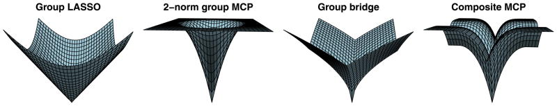
The group LASSO, group bridge and composite mcp penalties for a two-predictor group. Note that where the penalty comes to a point or edge, there is the possibility that the solution will take on a sparse value; all penalties come to a point at 0, encouraging group-level sparsity, but only group bridge and composite MCP allow for bi-level selection.

Figure 3 shows the coefficient paths from λ_max down to 0 for group LASSO, 1-norm group bridge, and composite MCP for a simulated data set featuring two groups, each with three covariates. In the underlying model, the group represented by solid lines has two covariates with coefficients equal to 1 and the other equal to 0; the group represented by dashed lines has two coefficients equal to 0 and the other equal to −1. The figure reveals much about the behavior of grouped penalties. In particular, we note the following: (1) Even though each of the nonzero coefficients is of the same magnitude, the coefficients from the more significant solid group enter the model more easily than the lone nonzero coefficient from the dashed group. (2) This phenomenon is less pronounced for composite MCP, which makes weaker assumptions about grouping. (3) For composite MCP at λ ≈ 0.3, all of the variables with true zero coefficients have been eliminated while the remaining coefficients are unpenalized. In this region, the composite MCP approach is performing as well as the oracle model. (4) In general, the coefficient paths for these group penalization methods are continuous, but are not piecewise linear, unlike those for the LASSO.

Fig. 3.

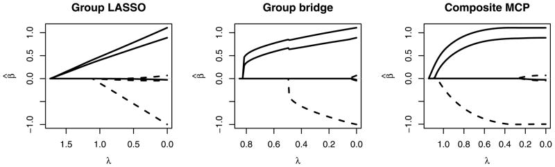
Coefficient paths from 0 to λ_MAX for group LASSO, 2-norm group MCP, 1-norm group bridge, and composite MCP for a simulated data set featuring two groups, each with three covariates. In the underlying data-generating mechanism, the group represented by solid lines has two covariates with coefficients equal to 1 and the other equal to 0; the group represented by dashed lines has two coefficients equal to 0 and the other equal to −1.

Although composite penalties do not, in general, have closed-form solutions in single-group models like the penalties in Section 2, the idea of group coordinate descent can still be used. The main complication is in step 2(b) for the algorithm described in Section 2.4, where the single-group solutions need to be solved numerically. Another approach is based on a local coordinate descent algorithm (Breheny and Huang, 2009). This algorithm first uses a local linear approximation to the penalty function (Zou and Li, 2008). After applying this approximation, in any given coordinate direction the optimization problem is equivalent to the one-dimensional LASSO, which has the soft-threshold operator as its solution. The thresholding parameter λ in each update is given by expression (3.4). Because the penalties involved are concave on [0, ∞), the linear approximation is a majorizing function, and the algorithm thus enjoys the descent property of MM algorithms (Lange, Hunter and Yang (2000)) whereby the objective function is guaranteed to decrease at every iteration. Further details may be found in Breheny and Huang (2009). These algorithms have been implemented in the R package grpreg, available at http://cran.r-project.org. The package computes the group LASSO, group bridge and composite MCP solutions for linear regression and logistic regression models.

3.3 Additive Penalties

Another approach to achieving bi-level selection is to add an ℓ₁ penalty to the group LASSO (Wu and Lange, 2008; Friedman, Hastie and Tibshirani, 2010).

$$\frac{1}{2n}{\Vert \mathbf{y}-\sum _{j=1}^J{X}_j{\mathit{\beta }}_j\Vert }_2^2+{\lambda }_1{\Vert {\mathit{\beta }}_1\Vert }_1+{\lambda }_2\sum _{j=1}^J{\Vert {\mathit{\beta }}_j\Vert }_2,$$ (3.6)

where λ₁ ≥ 0 and λ₂ ≥ 0 are regularization parameters. The above objective function has the benefit of being convex, eliminating the possibility of convergence to a local minimum during model fitting. The group coordinate descent algorithm can no longer be applied, however, as the orthonormalization procedure described in Section 2 will not preserve the sparsity achieved by the ℓ₁ penalty once the solution is transformed back to the original variables. Puig, Wiesel and Hero (2011), Friedman, Hastie and Tibshirani (2010) and Zhou et al. (2010) have proposed algorithms for solving this problem without requiring orthonormalization.

In principle, the group LASSO portion of the penalty could be replaced with any of the convex 2-norm group penalties of Section 2.2; likewise the ℓ₁ penalty could be replaced by, say, MCP or SCAD. These possibilities, to the best of our knowledge, have not been explored. Further work is needed to study the properties of this class of estimators and compare their performance with other methods.

3.4 Example: Genetic Association

We now give an example from a genetic association study where bi-level selection is an important goal of the study. The example involves data from a case-control study of age-related macular degeneration consisting of 400 cases and 400 controls, and was analyzed in Breheny and Huang (2009). The analysis is confined to 30 genes containing 532 markers that previous biological studies have suggested may be related to the disease.

We analyze the data with the group LASSO, 1-norm group bridge and composite MCP methods by considering markers to be grouped by the gene they belong to. Penalized logistic regression models were fit assuming an additive effect for all markers (homozygous dominant = 2, heterozygous = 1, homozygous recessive = 0). In addition to the group penalization methods, we analyzed these data using a traditional one-at-a-time approach (single-marker analysis), in which univariate logistic regression models were fit and marker effects screened using a p < 0.05 cutoff. Ten-fold cross-validation was used to select λ, and to assess accuracy (for the one-at-a-time approach, predictions were made from an unpenalized logistic regression model fit to the training data using all the markers selected by individual testing). The results are presented in Table 1.

Table 1.

Application of the three group penalization methods and a one-at-a-time method to a genetic association data set. CV error is the average number of misclassification errors over the ten validation folds

	Genes selected	Markers selected	Cross-validation error
One-at-a-time	19	49	0.441
Group LASSO	17	g	0.390
Group bridge	3	20	0.400
Composite MCP	8	11	0.391

Table 1 suggests the benefits of using group penalization regression approaches as opposed to one-at-a-time approaches: the three group penalization methods achieve lower test error rates and do so while selecting fewer genes (groups). Although the error rates of ≈40% indicate that these 30 genes likely do not include SNPs that exert a large effect on an individual’s chances of developing age-related macular degeneration, the fact that they are well below the 50% that would be expected by random chance demonstrates that these genes do contain SNPs related to the disease. The very different nature of the selection properties of the three group penalization methods are also clearly seen. Although group LASSO achieves low misclassification error, it selects 17 genes out of 30 and 435 markers out of 532, failing to shed light on the most important genetic markers. The bi-level selection methods achieve comparable error rates with a much more sparse set of predictors: group bridge identifies 3 promising genes out of 30 candidates, and composite MCP identifies 11 promising SNPs out of 532.

4. ORACLE PROPERTY OF THE 2-NORM GROUP MCP

In this section, we look at the selection properties of the 2-norm group MCP estimator β̂(λ, γ), defined as the global minimizer of (2.3) with $c_j=\sqrt{d_j}$, when ρ is taken to be the MCP penalty. We provide sufficient conditions under which the 2-norm group MCP estimator is equal to the oracle least squares estimator defined at (4.1) below. Our intention is to give some preliminary theoretical justification for this concave group selection method under reasonable conditions, not necessarily to obtain the best possible theoretical results or to provide a systematic treatment of the properties of the concave group selection methods discussed in this review.

Let X = (X₁, …, X_J) and Σ = X′X/n. For any A ⊆ {1, …, J}, denote

$$X_A=(X_j,j\in A),{\mathrm{\sum }}_A=X_A^{\prime }{X}_A/n.$$

Let the true value of the regression coefficients be ${\mathit{\beta }}^o={({{\mathit{\beta }}_1^o}^{\prime },\dots ,{{\mathit{\beta }}_J^o}^{\prime })}^{\prime }$. Let $S=\{j:{\Vert {\mathit{\beta }}_j^o\Vert }_2\ne 0,1\le j\le J\}$, which is the set of indices of the groups with nonzero coefficients in the underlying model. Let ${\beta }_{\ast }^o=min\{{\Vert {\mathit{\beta }}_j^o\Vert }_2/\sqrt{d_j}:j\in S\}$ and set ${\beta }_{\ast }^0=\infty$ if S is empty. Define

$${\widehat{\mathit{\beta }}}^o=\underset{b}{\text{argmin}}\{{\Vert \mathbf{y}-X\mathbf{b}\Vert }_2^2:{\mathbf{b}}_j=\mathbf{0}\forall j\notin S\}.$$ (4.1)

This is the oracle least squares estimator. Of course, it is not a real estimator, since the oracle set is unknown.

Let d_max = max{d_j: 1 ≤ j ≤ J} and d_min = min{d_j: 1 ≤ j ≤ J}. For any A ⊆ {1, …, J}, denote d_min(A) = min{d_j: j ∈ A} and d_max(A) = max{d_j: j ∈ A}. Here d_min(A) = ∞ if A is empty. Let c_min be the smallest eigenvalue of Σ, and let c₁ and c₂ be the smallest and largest eigenvalues of Σ_S, respectively.

We first consider the case where the 2-norm group MCP objective function is convex. This necessarily requires c_min > 0. Define the function

$$h(t,k)=exp(-k{(\sqrt{2t-1}-1)}^2/4),t>1,k=1,2,\dots .$$ (4.2)

This function arises from an upper bound for the tail probabilities of chi-square distributions given in Lemma A.1 in the Appendix, which is based on an exponential inequality for chi-square random variables of Laurent and Massart (2000). Let

$${\eta }_{1n}(\lambda )=(J-\mid S\mid )h({\lambda }^{2}n/{\sigma }^2,d_{min}(S^c))$$ (4.3)

and

$${\eta }_{2n}(\lambda )=\mid S\mid h(c_{1}n{({\beta }_{\ast }^o-\gamma \lambda )}^2/{\sigma }^2,d_{min}(S)).$$ (4.4)

Theorem 4.1

Suppose ε₁, …, ε_n are independent and identically distributed as N(0, σ²). Then for any (λ, γ) satisfying γ > 1/c_min, ${\beta }_{\ast }^o>\gamma \lambda$ and nλ² > σ², we have

$$\text{P}(\widehat{\mathit{\beta }}(\lambda ,\gamma )\ne {\widehat{\mathit{\beta }}}^o)\le {\eta }_{1n}(\lambda )+{\eta }_{2n}(\lambda ).$$

The proof of this theorem is given in the Appendix. It provides an upper bound on the probability that β̂(λ, γ) is not equal to the oracle least squares estimator. The condition γ > 1/c_min ensures that the 2-norm group MCP criterion is strictly convex. This implies β̂(λ, γ) is uniquely characterized by the Karush–Kuhn–Tucker conditions. The condition nλ² > σ² requires that λ cannot be too small.

Let

$$\begin{array}{l}{\lambda }_n=\sigma {(2log(max\{J-\mid S\mid ,1\})/({nd}_{min}(S^c)))}^{1/2}\text{and}\\ {\tau }_n=\sigma \sqrt{2log(max\{\mid S\mid ,1\})/({nc}_1{d}_{min}(S))}.\end{array}$$ (4.5)

The following corollary is an immediate consequence of Theorem 4.1.

Corollary 4.1

Suppose that the conditions of Theorem 4.1 are satisfied. Also suppose that ${\beta }_{\ast }^o\ge \gamma \lambda +a_n{\tau }_n$ for a_n → ∞ as n → ∞. If λ ≥ a_nλ_n, then

$$\text{P}(\widehat{\mathit{\beta }}(\lambda ,\gamma )\ne {\widehat{\mathit{\beta }}}^o)\to Oasn\to \infty .$$

By Corollary 4.1, the 2-norm group MCP estimator behaves like the oracle least squares estimator with high probability. This of course implies it is group selection consistent. For the standard LASSO estimator, a sufficient condition for its sign consistency is the strong irrepresentable condition (Zhao and Yu, 2006). Here a similar condition holds automatically due to the form of the MCP. Specifically, let ${\mathit{\beta }}_S^o={({{\mathit{\beta }}_j^o}^{\prime }:j\in S)}^{\prime }$. Then an extension of the irrepresentable condition to the present setting is, for some 0 < δ < 1,

$$\underset{j\notin S}{max}{\Vert X_j^{\prime }{X}_S{(X_S^{\prime }{X}_S)}^{-1}\stackrel{.}{\rho }({\mathit{\beta }}_S^o;\lambda ,\gamma )/\lambda \Vert }_2\le 1-\delta ,$$ (4.6)

where $\stackrel{.}{\rho }({\mathit{\beta }}_S^o;\lambda ,\gamma )={(\stackrel{.}{\rho }({\Vert {\mathit{\beta }}_j^o\Vert }_2;\sqrt{d_j}\lambda ,\gamma ){{\mathit{\beta }}_j^o}^{\prime }/{\Vert {\mathit{\beta }}_j^o\Vert }_{2}j\in S)}^{\prime }$ with

$$\stackrel{.}{\rho }({\Vert {\mathit{\beta }}_j^o\Vert }_2;\sqrt{d_j}\lambda ,\gamma )=\lambda {(1-{\Vert {\mathit{\beta }}_j^o\Vert }_2/(\sqrt{d_j}\gamma \lambda ))}_{+}.$$

Since it is assumed that ${min}_{j\in S}{\Vert {\mathit{\beta }}_j^o\Vert }_2/\sqrt{d_j}>\gamma \lambda$, we have $\stackrel{.}{\rho }({\Vert {\mathit{\beta }}_j^o\Vert }_2;\sqrt{d_j}\lambda ,\gamma )=0$ for all j ∈ S. Therefore, (4.6) always holds.

We now consider the high-dimensional case where J > n. We require the sparse Riesz condition, or SRC (Zhang and Huang, 2008), which is a form of sparse eigenvalue condition. We say that X satisfies the SRC with rank d^* and spectrum bounds {c_*, c^*} if

$$0<c_{\ast }\le {\Vert X_A\mathbf{u}\Vert }_2^2/n\le c^{\ast }<\infty \forall A\text{with}\mid A\mid \le d^{\ast },{\Vert \mathbf{u}\Vert }_2=1.$$ (4.7)

We refer to this condition as SRC(d^*, c_*, c^*).

Let K_* = (c^*/c_*) − (1/2), m_* = K_*|S| and ξ = 1/(4c^*d_s), where d_s = max{d_max(S), 1}. Define

$${\eta }_{3n}(\lambda )={(J-\mid S\mid )}^{m_{\ast }}\frac{e^{m_{\ast }}}{m_{\ast }^{m_{\ast }}}·h(\xi n{\lambda }^2{\sigma }^{-2}/d_{max},m_{\ast }{d}_{max}).$$ (4.8)

Let η_1n and η_2n be as in (4.3) and (4.4).

Theorem 4.2

Suppose ε₁, …, ε_n are independent and identically distributed as N(0, σ²), and X satisfies the SRC(d^*, c_*, c^*) in (4.7) with d^* ≥ (K_* + 1) |S|d_s. Then for any (λ, γ) satisfying ${\beta }_{\ast }^o>\gamma \lambda$, nλ²ξ > σ² d_max and $\gamma \ge c_{\ast }^{-1}\sqrt{4+(c_{\ast }/c^{\ast })}$, we have

$$\mathbf{P}(\widehat{\mathit{\beta }}(\lambda ,\gamma )\ne {\widehat{\mathit{\beta }}}^o)\le {\eta }_{1n}(\lambda )+{\eta }_{2n}(\lambda )+{\eta }_{3n}(\lambda ).$$

Letting

$${\lambda }_n^{\ast }=2\sigma \sqrt{2c^{\ast }{d}_{s}log(J-\mid S\mid )/n}$$

and τ_n be as in (4.5), Theorem 4.2 has the following corollary.

Corollary 4.2

Suppose the conditions of Theorem 4.2 are satisfied. Also suppose ${\beta }_{\ast }^o\ge \gamma \lambda +a_n{\tau }_n$ for a_n → ∞ as n → ∞. Then if $\lambda \ge a_n{\lambda }_n^{\ast }$,

$$\text{P}(\widehat{\mathit{\beta }}(\lambda ,\gamma )\ne {\stackrel{\sim }{\mathit{\beta }}}^o)\to 0asn\to \infty .$$

Theorem 4.2 and Corollary 4.2 provide sufficient conditions for the selection consistency of the global 2-norm group MCP estimator in the J ≫ n situations. For example, we can have J − |S| = exp{o(n/(c^* d_s))}. The condition nλ²ξ > σ²d_max is stronger than the corresponding condition nλ² > σ² in Theorem 4.1. The condition $\gamma \ge c_{\ast }^{-1}\sqrt{4+(c_{\ast }/c^{\ast })}$ ensures that the group MCP criterion is convex in any d^*-dimensional subspace. It is stronger than the minimal sufficient condition γ > 1/c_* for convexity in d^*-dimensional subspaces. These reflect the difficulty and extra efforts needed in reducing a p-dimensional problem to a d^*-dimensional problem. The SRC in (4.7) guarantees that the model is identifiable in a lower d^*-dimensional space.

The results presented above are concerned with the global solutions. The properties of the local solutions, such as those produced by the group coordinate descent algorithm, to concave 2-norm or 1-norm penalties remain largely unknown in models with J ≫ n. An interesting question is under what conditions the local solutions are equal to or sufficiently close to the global solutions so that they are still selection consistent. In addition, the estimation and prediction properties of these solutions have not been studied. We expect that the methods of Zhang and Zhang (2011) in studying the properties of concave regularization will be helpful in group and bi-level selection problems.

5. APPLICATIONS

We now give a review of some applications of the group selection methods in several statistical modeling and analysis problems, including nonparametric additive models, semiparametric partially linear models, seemingly unrelated regressions and multitask learning and genetic and genomic data analysis.

5.1 Nonparametric Additive Models

Let (y_i, x_i), i = 1, …, n be random vectors that are independently and identically distributed as (y, x), where y is a response variable, and x = (x₁, …, x_p)′ is a p-dimensional covariate vector. The nonparametric additive model (Hastie and Tibshirani, 1990) posits that

$$y_i=\mu +\sum _{j=1}^p{f}_j(x_{ij})+{\epsilon }_i,1\le i\le n,$$ (5.1)

where μ is an intercept term, x_ij is the jth component of x_i, the f_j’s are unknown functions and ε_i is an unobserved random variable with mean zero and finite variance σ². Suppose that some of the additive components f_j are zero. The problem is to select the nonzero components and estimate them. Lin and Zhang (2006) proposed the component selection and smoothing operator (COSSO) method that can be used for selection and estimation in (5.1). The COSSO can be viewed as a group LASSO procedure in a reproducing kernel Hilbert space. For fixed p, they studied the rate of convergence of the COSSO estimator in the additive model. They also showed that, in the special case of a tensor product design, the COSSO correctly selects the non-zero additive components with high probability. Zhang and Lin (2006) considered the COSSO for nonparametric regression in exponential families. Meier, van de Geer and Bühlmann (2009) proposed a variable selection method in (5.1) with p ≫ n that is closely related to the group LASSO. They give conditions under which, with high probability, their procedure selects a set of the nonparametric components whose distance from zero in a certain metric exceeds a specified threshold under a compatibility condition. Ravikumar et al. (2009) proposed a penalized approach for variable selection in (5.1). In their theoretical results on selection consistency, they assume that the eigenvalues of a “design matrix” be bounded away from zero and infinity, where the “design matrix” is formed from the basis functions for the nonzero components. Another critical condition required in their paper is similar to the irrepresentable condition of Zhao and Yu (2006). Huang, Horowitz and Wei (2010) studied the group LASSO and adaptive group LASSO for variable selection in (5.1) based on a spline approximation to the nonparametric components. With this approximation, each nonparametric component is represented by a linear combination of spline basis functions. Consequently, the problem of component selection becomes that of selecting the groups of coefficients in the linear combinations. They provided conditions under which the group LASSO selects a model whose number of components is comparable with the underlying model, and the adaptive group LASSO selects the nonzero components correctly with high probability and achieves the optimal rate of convergence.

5.2 Structure Estimation in Semiparametric Regression Models

Consider the semiparametric partially linear model (Engle et al., 1986)

$$y_i=\mu +\sum _{j\in S_1}{\beta }_j{x}_{ij}+\sum _{j\in S_2}{f}_j(x_{ij})+{\epsilon }_i,1\le i\le n,$$ (5.2)

where S₁ and S₂ are mutually exclusive and complementary subsets of {1, …, p}, {β_j: j ∈ S₁} are regression coefficients of the covariates with indices in S₁ and (f_j: j ∈ S₂) are unknown functions. The most important assumption in the existing methods for the estimation in partially linear models is that S₁ and S₂ are known a priori. This assumption underlies the construction of the estimators and investigation of their theoretical properties in the existing methods (Härdle, Liang and Gao, 2000; Bickel et al., 1993). However, in applied work, it is rarely known in advance which covariates have linear effects and which have nonlinear effects. Recently, Zhang, Cheng and Liu (2011) proposed a method for determining the zero, linear and nonlinear components in partially linear models. Their method is a regularization method in the smoothing spline ANOVA framework that is closely related to the COSSO. They obtained the rate of convergence of their proposed estimator. They also showed that their method is selection consistent in the special case of tensor product design. But their approach requires tuning of four penalty parameters, which may be difficult to implement in practice. Huang, Wei and Ma (2011) proposed a semiparametric regression pursuit method for estimating S₁ and S₂. They embedded partially linear models into model (5.1). By approximating the nonparametric components using spline series expansions, they transformed the problem of model specification into a group variable selection problem. They then used the 2-norm group MCP to determine the linear and nonlinear components. They showed that, under suitable conditions, the proposed approach is consistent in estimating the structure of (5.2), meaning that it can correctly determine which covariates have a linear effect and which do not with high probability.

5.3 Varying Coefficient Models

Consider the linear varying coefficient model

$$y_i(t_{ij})=\sum _{k=1}^p{x}_{ik}(t_{ij}){\beta }_k(t_{ij})+{\epsilon }_i(t_{ij}),i=1,\dots ,n,j=1,\dots ,n_i,$$

where y_i(t) is the response variable for the ith subject at time point t ∈ T with T being the time interval on which the measurements are taken, ε_i(t) is the error term, x_ik(t)’s are time-varying covariates, β_k(t) is the corresponding smooth coefficient function. Such a model is useful in investigating the time-dependent effects of covariates on responses measured repeatedly. One well-known example is longitudinal data analysis (Hoover et al., 1998) where the response for the ith experimental subject in the study is observed n_i occasions, the set of observations at times {t_ij: j = 1, …, n_i} tends to be correlated. Another important example is the functional response models (Rice, 2004), where the response y_i(t) is a smooth real function, although only y_i(t_ij), j = 1, …, n_i are observed in practice. Wang, Chen and Li (2007) and Wang and Xia (2009) considered the use of group LASSO and SCAD methods for model selection and estimation in (5.3). Xue, Qu and Zhu (2010) applied the 2-norm SCAD method for variable selection in generalized linear varying-coefficient models and considered its selection and estimation properties. These authors obtained their results in the models with fixed dimensions. Wei, Huang and Li (2011) studied the properties of the group LASSO and adaptive group LASSO for (5.3) in the p ≫ n settings. They showed that, under the sparse Riesz condition and other regularity conditions, the group LASSO selects a model of the right order of dimensionality, selects all variables with co-efficient functions whose ℓ₂ norm is greater than a certain threshold level and is estimation consistent. They also proved that the adaptive group LASSO can correctly select important variables with high probability based on an initial consistent estimator.

5.4 Seemingly Unrelated Regressions and Multi-Task Learning

Consider T linear regression models

$${\mathbf{y}}_t=X_t{\mathit{\beta }}_t+{\mathit{\epsilon }}_t,t=1,\dots ,T,$$

where y_t is an n × 1 response vector, X_t is an n × p design matrix, β_t is a p × 1 vector of regression co-efficients and ε_t is an n × 1 error vector. Assume that ε₁, …, ε_T are independent and identically distributed with mean zero and covariance matrix Σ. This model is referred to as the seemingly unrelated regressions (SUR) model (Zellner, 1962). Although each model can be estimated separately based on least squares method, it is possible to improve on the estimation efficiency of this approach. Zellner (1962) proposed a method for estimating all the coefficients simultaneously that is more efficient than the single-equation least squares estimators. This model is also called a multi-task learning model in machine learning (Caruana, 1997; Argyriou, Evgeniou and Pontil, 2008).

Several authors have considered the problem of variable selection based on the criterion

$$\frac{1}{2T}\sum _{t=1}^T\frac{1}{n}{\Vert {\mathbf{y}}_t-X_t{\mathit{\beta }}_t\Vert }_2^2+\lambda \sum _{j=1}^p{\left(\sum _{t=1}^T{\beta }_{tj}^2\right)}^{1/2}.$$

This is a special case of the general group LASSO criterion. Here the groups are formed by the co-efficients corresponding to the jth variable across the regressions. The assumption here is that the jth variable plays a similar role across the tasks and should be selected or dropped at the same time. Several authors have studied the selection, estimation and prediction properties of the group LASSO in this model; see, for example, Bach (2008), Lounici et al. (2009), Lounici et al. (2011) and Obozinski, Wainwright and Jordan (2011) under various conditions on the design matrices and other regularity conditions.

5.5 Analysis of Genomic Data

Group selection methods have important applications in the analysis of high throughput genomic data—for example, to find genes and genetic pathways that affect a clinical phenotype such as disease status or survival using gene expression data. Most phenotypes are the result of alterations in a limited number of pathways, and there is coordination among the genes in these pathways. The genes in the same pathway or functional group can be treated as a group. Efficiency may be improved upon by incorporating pathway information into the analysis, thereby selecting pathways and genes simultaneously. Another example is integrative analysis of multiple genomic datasets. In gene profiling studies, markers identified from analysis of single datasets often suffer from a lack of reproducibility. Among the many possible causes, the most important one is perhaps the relatively small sample sizes and hence lack of power of individual studies. A cost-effective remedy to the small sample size problem is to pool and analyze data from multiple studies of the same disease. A generalized seemingly unrelated regressions model can be used in this context, where a group structure arises naturally for the multiple measurements for the same gene across the studies. Some examples of using group selection methods in these applications include Wei and Li (2007), Jacob, Obozinski and Vert (2009), Ma and Huang (2009), Ma, Huang and Moran (2009), Ma, Huang and Song (2010), Ma et al. (2011), Pan, Xie and Shen (2010) and Peng et al. (2010), among others.

5.6 Genome Wide Association Studies

Genome wide association studies (GWAS) are an important method for identifying disease susceptibility genes for common and complex diseases. GWAS involve scanning hundreds to thousands of samples, often as case-control samples, utilizing hundreds of thousands of single nucleotide polymorphism (SNP) markers located throughout the human genome. The SNPs from the same gene can be naturally considered as a group. It is more powerful to select both SNPs and genes simultaneously than to select them separately. Applications of group selection methods to genetic association analysis are discussed in Breheny and Huang (2009) and Zhou et al. (2010).

6. DISCUSSION

In this article, we provide a selective review of several group selection and bi-level selection methods. While considerable progress has been made in this area, much work remains to be done on a number of important issues. Here we highlight some of them that require further study in order to better apply these methods in practice.

6.1 Penalty Parameter Selection

In any penalization approach for variable selection, a difficult question is how to determine the penalty parameters. This question is even more difficult in group selection methods. Widely used criterions, including the AIC (Akaike, 1973) and BIC (Schwarz, 1978), require the estimation of the error variance and degrees of freedom. For the group LASSO, Yuan and Lin (2006) proposed an estimate of the degrees of freedom, but it involves the least squares estimator of the coefficients, which is not feasible in p ≫ n models. The problem of variance estimation has not been studied systematically in group selection models. It is possible to use K-fold cross validation, which does not require estimating the variance or the degrees of freedom. However, to our knowledge, there have been no rigorous analyses of this procedure in group selection settings. Recently, Meinshausen and Bühlmann (2010) proposed stability selection for choosing penalty parameters based on resampling. This is a general approach and is applicable to the group selection methods discussed here. Furthermore, it does not require estimating the variance or the degrees of freedom. It would be interesting to apply this method to group selection and compare it with the existing methods in group selection problems.

6.2 Theoretical Properties

Currently, most theoretical results concerning selection, estimation and prediction on group selection methods in p ≫ n settings are derived for the group LASSO in the context of linear regression. These results provide important insights into the behavior of the group LASSO. However, they are obtained for a given range of the penalty parameter. It is not clear whether, if the penalty parameter is selected using a data-driven procedure, such as cross validation, these results still hold. It is clearly of practical interest to confirm the estimation and prediction properties of group LASSO if the penalty parameter is selected using such a procedure. For concave selection methods, we considered the selection property of the global 2-norm group MCP solutions. Although global results shed some light on the properties of these methods, it is more relevant to investigate the properties of the local solutions, such as those obtained based on the group coordinate descent algorithm. Therefore, much work is needed to understand the theoretical properties of various concave group selection methods and compare their performance with the group LASSO.

6.3 Overlapping Groups

In this article, we only considered the case where there is no overlapping among the groups. However, in many applied problems, overlapped groups arise naturally. For example, in genomic data analysis involving genes and pathways, many important genes belong to multiple pathways. Jacob, Obozinski and Vert (2009) proposed an extended group LASSO method for selection with overlapping groups. With their method, it is possible to select one variable without selecting all the groups containing it. Percival (2011) studied the theoretical properties of the method of Jacob, Obozinski and Vert (2009). Liu and Ye (2010) proposed an algorithm for solving the overlapping group LASSO problem. Zhao, Rocha and Yu (2009) considered the problem of overlapping groups in the context of composite absolute penalties. The results of Huang et al. (2009) on the selection consistency of the 1-norm group bridge allow overlapping among groups under the assumption that the extent of overlapping is not large. However, in general, especially for concave group selection methods, this question has not been addressed.

APPENDIX

Lemma A.1

Let ${\chi }_k^2$ be a random variable with chi-square distribution with k degrees of freedom. For t > 1, $\text{P}({\chi }_k^2\ge kt)\le h(t,k)$, where h(t, k) is defined in (4.2).

This lemma is a restatement of the exponential inequality for chi-square distributions of Laurent and Massart (2000).

Proof of Theorem 4.1

Since β̂^o is the oracle least squares estimator, we have ${\widehat{\mathit{\beta }}}_j^o=0$ for j ∉ S and

$$-X_j^{\prime }(\mathbf{y}=X{\widehat{\mathit{\beta }}}^o)/n=0\forall j\in S.$$ (A.1)

If ${\Vert {\widehat{\mathit{\beta }}}_j^o\Vert }_2/\sqrt{d_j}\ge \gamma \lambda$, then by the definition of the MCP, ${\rho }^{\prime }({\Vert {\widehat{\mathit{\beta }}}_j^o\Vert }_2;\sqrt{d_j}\lambda ,\gamma )=0$. Since c_min > 1/γ, the criterion (2.3) is strictly convex. By the KKT conditions, the equality β̂(λ, γ) = β̂^o holds in the intersection of the events

$$\begin{array}{l}{\mathrm{\Omega }}_1(\lambda )=\left\{\underset{j\notin S}{max}{\Vert n^{-1}{X}_j^{\prime }(\mathbf{y}-X{\widehat{\mathit{\beta }}}^o)\Vert }_2/\sqrt{d_j}\le \lambda \right\}\text{and}\\ {\mathrm{\Omega }}_2(\lambda )=\left\{\underset{j\in S}{min}{\Vert {\widehat{\mathit{\beta }}}_j^o\Vert }_2/\sqrt{d_j}\ge \gamma \lambda \right\}.\end{array}$$ (A.2)

We first bound 1 − P(Ω₁(λ)). Let β̂_S = (β̂_j, j ∈ S)′. By (A.1) and using $\mathbf{y}=X_S{\mathit{\beta }}_S^o+\epsilon$,

$${\widehat{\mathit{\beta }}}_S^o={\mathrm{\sum }}_S^{-1}{X}_S^{\prime }\mathbf{y}/n={\mathit{\beta }}_S^o+{\mathrm{\sum }}_S^{-1}{X}_S^{\prime }\mathit{\epsilon }/n.$$ (A.3)

It follows that $n^{-1}{X}_j^{\prime }(\mathbf{y}-X{\widehat{\mathit{\beta }}}^o)=n^{-1}{X}_j^{\prime }(I_n-P_S)\mathit{\epsilon }$, where $P_S=n^{-1}{X}_S{\mathrm{\sum }}_S^{-1}{X}_S^{\prime }$. Because $X_j^{\prime }{X}_j=I_{d_j},{\Vert X_j^{\prime }(I_n-P_S)\mathit{\epsilon }\Vert }_2^2/{\sigma }^2$ is distributed as a χ² distribution with d_j degrees of freedom. We have, for nλ²/σ² ≥ 1,

$$\begin{array}{l}1-\text{P}({\mathrm{\Omega }}_1(\lambda ))=\text{P}\left(\underset{j\notin S}{max}{\Vert n^{-1/2}{X}_j^{\prime }(I_n-P_S)\mathit{\epsilon }\Vert }_2^2/(d_j{\sigma }^2)>n{\lambda }^2/{\sigma }^2\right)\\ \le \sum _{j\notin S}\text{P}({\Vert n^{-1/2}{X}_j^{\prime }(I_n-P_S)\mathit{\epsilon }\Vert }_2^2/{\sigma }^2>d_{j}n{\lambda }^2/{\sigma }^2)\\ \le \sum _{j\notin S}h(n{\lambda }^2/{\sigma }^2,d_j)\\ \le (J-\mid S\mid )h(n{\lambda }^2/{\sigma }^2,d_{min}(S^c))\\ ={\eta }_{1n}(\lambda ),\end{array}$$ (A.4)

where we used Lemma A.1 in the third line.

Now consider Ω₂. Recall ${\beta }_{\ast }^o={min}_{j\in S}{\Vert {\mathit{\beta }}_j^o\Vert }_2/\sqrt{d_j}$. If ${\Vert {\widehat{\mathit{\beta }}}_j^o-{\mathit{\beta }}_j^o\Vert }_2/\sqrt{d_j}\le {\beta }_{\ast }^o-\gamma \lambda$ for all j ∈ S, then ${min}_{j\in S}{\Vert {\widehat{\mathit{\beta }}}_j^o\Vert }_2/\sqrt{d_j}\ge \gamma \lambda$. This implies

$$1-\text{P}({\mathrm{\Omega }}_2(\lambda ))\le \text{P}\left(\underset{j\in S}{max}{\Vert {\widehat{\mathit{\beta }}}_j^o-{\mathit{\beta }}_j^o\Vert }_2/\sqrt{d_j}>{\beta }_{\ast }^o-\gamma \lambda \right).$$

Let A_j be a d_j × d_S matrix with a d_j × d_j identity matrix I_dj in the jth block and 0’s elsewhere. Then $n^{1/2}({\widehat{\mathit{\beta }}}_j^o-{\mathit{\beta }}_j^o)=n^{-1/2}{A}_j{\mathrm{\sum }}_S^{-1}{X}_S^{\prime }\mathit{\epsilon }$. Note that

$$\begin{array}{l}{\Vert n^{-1/2}{A}_j{\mathrm{\sum }}_S^{-1}{X}_S^{\prime }\mathit{\epsilon }\Vert }_2\le {\Vert A_j\Vert }_2{\Vert {\mathrm{\sum }}_S^{-1/2}\Vert }_2{\Vert n^{-1/2}{\mathrm{\sum }}_S^{-1/2}{X}_S^{\prime }\mathit{\epsilon }\Vert }_2\\ \le c_1^{-1/2}{\Vert n^{-1/2}{\mathrm{\sum }}_S^{-1/2}{X}_S^{\prime }\mathit{\epsilon }\Vert }_2\end{array}$$

and ${\Vert n^{-1/2}{\mathrm{\sum }}_S^{-1/2}{X}_S^{\prime }\mathit{\epsilon }\Vert }_2^2/{\sigma }^2$ is distributed as a χ² distribution with |S| degrees of freedom. Therefore, similar to (A.4), we have, for $c_{1}n{({\beta }_{\ast }^o-\gamma \lambda )}^2/{\sigma }^2>1$,

$$\begin{array}{l}1-\text{P}({\mathrm{\Omega }}_2(\lambda ))=\text{P}\left(\underset{j\in S}{max}{n}^{-1/2}{\Vert A_j{\mathrm{\sum }}_S^{-1}{X}_S^{\prime }\epsilon \Vert }_2/\sqrt{d_j}>\sqrt{n}({\beta }_{\ast }^o-\gamma \lambda )\right)\\ \le \text{P}\left(\underset{j\in S}{max}{\Vert n^{-1/2}{\mathrm{\sum }}_S^{-1/2}{X}_S^{\prime }\mathit{\epsilon }\Vert }_2^2/(d_j{\sigma }^2)>c_{1}n{({\beta }_{\ast }^o-\gamma \lambda )}^2/{\sigma }^2\right)\\ \le \mid S\mid h(c_{1}n{({\beta }_{\ast }^o-\gamma \lambda )}^2/{\sigma }^2,d_{min}(S))\\ ={\eta }_{2n}(\lambda ).\end{array}$$ (A.5)

Combining (A.4) and (A.5), we have

$$\begin{array}{l}\text{P}(\widehat{\mathit{\beta }}(\lambda ,\gamma )\ne {\widehat{\mathit{\beta }}}^o)\le 1-\text{P}({\mathrm{\Omega }}_1(\lambda ))+1-\text{P}({\mathrm{\Omega }}_2(\lambda ))\\ \le {\eta }_{1n}(\lambda )+{\eta }_{2n}(\lambda ).\end{array}$$

This completes the proof.

For any B ⊂ {1, …, J} and m ≥ 1, define

$$\zeta (v;m,B)=max\left\{\frac{{\Vert (P_A-P_B)v\Vert }_2}{{(mn)}^{1/2}}:B\subseteq A\subseteq \{1,\dots ,J\},d_A=m+d_B\right\}$$ (A.6)

for υ ∈ ℝⁿ, where $P_A=X_A{(X_A^{\prime }{X}_A)}^{-1}{X}_A^{\prime }$ is the orthogonal projection from ℝⁿ to the span of X_A.

Lemma A.2

Suppose ξnλ² > σ²d_max. We have

$$\text{P}(2\sqrt{c^{\ast }{d}_s}\zeta (\mathbf{y};m,S)>\lambda )\le {(J-\mid S\mid )}^m\frac{e^m}{m^m}exp(-m\xi n{\lambda }^2/16).$$

Proof

For any A ⊇ S, we have (P_A − P_S) X_Sβ_S = 0. Thus

$$(P_A-P_S)\mathbf{y}=(P_A-P_{A_S})(X_S{\mathit{\beta }}_S+\epsilon )=(P_A-P_S)\epsilon .$$

Therefore,

$$\text{P}(2\sqrt{c^{\ast }{d}_s}\zeta (\mathbf{y};m,S)>\lambda )=\text{P}\left(\underset{A\supseteq S,\mid A\mid -\mid S\mid =m}{max}{\Vert (P_A-P_S)\epsilon \Vert }^2/{\sigma }^2>\xi mn{\lambda }^2\right).$$

Since P_A − P_S is a projection matrix, ${\Vert (P_A-P_S)\epsilon \Vert }^2/{\sigma }^2~{\chi }_{m_A}^2$, where m_A = Σ_{j∈A−S,A⊇S} d_j ≤ md_max. Since there are $\left(\begin{array}{c}J-\mid S\mid \\ m\end{array}\right)$ ways to choose A from {1, …, J}, we have

$$\text{P}(2\sqrt{c^{\ast }{d}_s}\zeta (\mathbf{y};m,S)>\lambda )\le \left(\begin{array}{c}J-\mid S\mid \\ m\end{array}\right)\text{P}({\chi }_{m{d}_{max}}^2>\xi mn{\lambda }^2).$$

This and Lemma A.1 imply that

$$\begin{array}{l}\text{P}(2\sqrt{c^{\ast }{d}_s}\zeta (\mathbf{y};m,S)>\lambda )\le \left(\begin{array}{c}J-\mid S\mid \\ m\end{array}\right)h(\xi n{\lambda }^2/d_{max},m{d}_{max})\\ \le {(J-\mid S\mid )}^m\frac{e^m}{m^m}h(\xi n{\lambda }^2/d_{max},m{d}_{max}).\end{array}$$

Here we used the inequality $\left(\begin{array}{c}J-\mid S\mid \\ m\end{array}\right)\le e^m{(J-\mid S\mid )}^m/m^m$. This completes the proof.

Define T as any set that satisfies

$$S\cup \{j:{\Vert {\widehat{\mathit{\beta }}}_j\Vert }_2\ne 0\}\subseteq T\subseteq S\cup \{j:n^{-1}{X}_j^{\prime }(\mathbf{y}-X\widehat{\mathit{\beta }})=\stackrel{.}{\rho }({\Vert {\widehat{\mathit{\beta }}}_j\Vert }_2;\sqrt{d_j}\lambda ,\gamma )·\sqrt{d_j}{\widehat{\mathit{\beta }}}_j/{\Vert {\widehat{\mathit{\beta }}}_j\Vert }_2\}.$$

Lemma A.3

Suppose that X satisfies the SRC(d^*, c_*, c^*), d^* ≥ (K_* + 1)|S|d_s, and $\gamma \ge c_{\ast }^{-1}·\sqrt{4+c_{\ast }/c^{\ast }}$. Let m_* = K_*|S|. Then for any y ∈ ℝⁿ with $\lambda \ge 2\sqrt{c^{\ast }{d}_s}\zeta (\mathbf{y};m_{\ast },S)$, we have

$$\mid T\mid \le (K_{\ast }+1)\mid S\mid .$$

Proof

This lemma can be proved along the line of the proof of Lemma 1 of Zhang (2010a) and is omitted.

Proof of Theorem 4.2

By Lemma A.3, in the event

$$2\sqrt{c^{\ast }{d}_{max}(S)}\zeta (\mathbf{y};m_{\ast },S)\le \lambda ,$$ (A.7)

we have |T| ≤ (K_* + 1)|S|. Thus in event (A.7), the original model with J groups reduces to a model with at most (K_* + 1)|S| groups. In this reduced model, the conditions of Theorem 4.2 imply that the conditions of Theorem 4.1 are satisfied. By Lemma A.2,

$$\text{P}(2\sqrt{c^{\ast }{d}_{max}(S)}\zeta (\mathbf{y};m_{\ast },S)>\lambda )\le {\eta }_{3n}(\lambda ).$$ (A.8)

Therefore, combining (A.8) and Theorem 4.1, we have

$$\text{P}(\widehat{\mathit{\beta }}(\lambda ,\gamma )\ne {\widehat{\mathit{\beta }}}^o)\le {\eta }_{1n}(\lambda )+{\eta }_{2n}(\lambda )+{\eta }_{3n}(\lambda ).$$

This proves Theorem 4.2.

References

- Akaike H. Second International Symposium on Information Theory (Tsahkadsor, 1971) Akadémiai Kiadó; Budapest: 1973. Information theory and an extension of the maximum likelihood principle; pp. 267–281. MR0483125. [Google Scholar]
- Antoniadis A. Smoothing noisy data with tapered coiflets series. Scand J Statist. 1996;23:313–330. [Google Scholar]
- Antoniadis A, Fan J. Regularization of wavelet approximations. J Amer Statist Assoc. 2001;96:939–967. [Google Scholar]
- Argyriou A, Evgeniou T, Pontil M. Convex multi-task feature learning. Mach Learn. 2008;73:243–272. [Google Scholar]
- Bach FR. Consistency of the group lasso and multiple kernel learning. J Mach Learn Res. 2008;9:1179–1225. [Google Scholar]
- Bakin S. PhD thesis. Australian National Univ; Canberra: 1999. Adaptive regression and model selection in data mining problems. [Google Scholar]
- Bickel PJ, Ritov Y, Tsybakov AB. Simultaneous analysis of lasso and Dantzig selector. Ann Statist. 2009;37:1705–1732. [Google Scholar]
- Bickel PJ, Klaassen CAJ, Ritov Y, Wellner JA. Efficient and Adaptive Estimation for Semiparametric Models. Johns Hopkins Univ. Press; Baltimore, MD: 1993. [Google Scholar]
- Breheny P, Huang J. Penalized methods for bi-level variable selection. Stat Interface. 2009;2:369–380. doi: 10.4310/sii.2009.v2.n3.a10. [DOI] [PMC free article] [PubMed] [Google Scholar]
- Breheny P, Huang J. Coordinate descent algorithms for nonconvex penalized regression, with applications to biological feature selection. Ann Appl Stat. 2011;5:232–253. doi: 10.1214/10-AOAS388. [DOI] [PMC free article] [PubMed] [Google Scholar]
- Bühlmann P, van de Geer S. Statistics for High-dimensional Data: Methods, Theory and Applications. Springer; Heidelberg: 2011. [Google Scholar]
- Caruana R. Multitask learning: A knowledge-based source of inductive bias. Machine Learning. 1997;28:41–75. [Google Scholar]
- Donoho DL, Johnstone IM. Ideal spatial adaptation by wavelet shrinkage. Biometrika. 1994;81:425–455. [Google Scholar]
- Efron B, Hastie T, Johnstone I, Tibshirani R. Least angle regression. Ann Statist. 2004;32:407–499. [Google Scholar]
- Engle RF, Granger CWJ, Rice J, Weiss A. Semiparametric estimates of the relation between weather and electricity sales. J Amer Statist Assoc. 1986;81:310–320. [Google Scholar]
- Fan J, Li R. Variable selection via nonconcave penalized likelihood and its oracle properties. J Amer Statist Assoc. 2001;96:1348–1360. [Google Scholar]
- Fan J, Peng H. Nonconcave penalized likelihood with a diverging number of parameters. Ann Statist. 2004;32:928–961. [Google Scholar]
- Frank IE, Friedman JH. A statistical view of some chemometrics regression tools (with discussion) Technometrics. 1993;35:109–148. [Google Scholar]
- Friedman J, Hastie T, Tibshirani R. A note on the group lasso and a sparse group lasso. 2010. Preprint, Dept. Statistics, Stanford Univ. [Google Scholar]
- Friedman J, Hastie T, Höfling H, Tibshirani R. Pathwise coordinate optimization. Ann Appl Stat. 2007;1:302–332. [Google Scholar]
- Fu WJ. Penalized regressions: The bridge versus the lasso. J Comput Graph Statist. 1998;7:397–416. [Google Scholar]
- Härdle W, Liang H, Gao J. Contributions to Statistics. Physica; Heidelberg: 2000. Partially Linear Models. [Google Scholar]
- Hastie TJ, Tibshirani RJ. Generalized Additive Models. Monographs on Statistics and Applied Probability. Vol. 43. Chapman & Hall; London: 1990. [Google Scholar]
- Hoover DR, Rice JA, Wu CO, Yang L-P. Nonparametric smoothing estimates of time-varying coefficient models with longitudinal data. Biometrika. 1998;85:809–822. [Google Scholar]
- Huang J, Horowitz JL, Ma S. Asymptotic properties of bridge estimators in sparse high-dimensional regression models. Ann Statist. 2008;36:587–613. [Google Scholar]
- Huang J, Horowitz JL, Wei F. Variable selection in nonparametric additive models. Ann Statist. 2010;38:2282–2313. doi: 10.1214/09-AOS781. [DOI] [PMC free article] [PubMed] [Google Scholar]
- Huang J, Wei F, Ma S. Semiparametric regression pursuit. Statist Sinica. 2011 doi: 10.5705/ss.2010.298. To appear. [DOI] [PMC free article] [PubMed] [Google Scholar]
- Huang J, Zhang T. The benefit of group sparsity. Ann Statist. 2010;38:1978–2004. [Google Scholar]
- Huang J, Ma S, Xie H, Zhang C-H. A group bridge approach for variable selection. Biometrika. 2009;96:339–355. doi: 10.1093/biomet/asp020. [DOI] [PMC free article] [PubMed] [Google Scholar]
- Jacob L, Obozinski G, Vert JP. Group lasso with overlap and graph lasso. Proceedings of the 26th Annual International Conference on Machine Learning; New York: ACM; 2009. pp. 433–440. [Google Scholar]
- Koltchinskii V. The Dantzig selector and sparsity oracle inequalities. Bernoulli. 2009;15:799–828. [Google Scholar]
- Lange K, Hunter DR, Yang I. Optimization transfer using surrogate objective functions. J Comput Graph Statist. 2000;9:1–59. [Google Scholar]
- Laurent B, Massart P. Adaptive estimation of a quadratic functional by model selection. Ann Statist. 2000;28:1302–1338. [Google Scholar]
- Leng C, Lin Y, Wahba G. A note on the lasso and related procedures in model selection. Statist Sinica. 2006;16:1273–1284. [Google Scholar]
- Lin Y, Zhang HH. Component selection and smoothing in multivariate nonparametric regression. Ann Statist. 2006;34:2272–2297. [Google Scholar]
- Liu J, Ye J. Fast overlapping group Lasso. 2010 Available at http://arxiv.org/abs/1009.0306.
- Lounici K, Pontil M, Tsybakov AB, van de Geer S. Taking advantage of sparsity in multitask learning. Knowledge and Information Systems. 2009;20:109–348. [Google Scholar]
- Lounici K, Pontil M, van de Geer S, Tsybakov AB. Oracle inequalities and optimal inference under group sparsity. Ann Statist. 2011;39:2164–2204. [Google Scholar]
- Ma S, Huang J. Regularized gene selection in cancer microarray meta-analysis. BMC Bioinformatics. 2009;10:1. doi: 10.1186/1471-2105-10-1. [DOI] [PMC free article] [PubMed] [Google Scholar]
- Ma S, Huang J, Moran MS. Identification of genes associated with multiple cancers via integrative analysis. BMC Genomics. 2009;10:535. doi: 10.1186/1471-2164-10-535. [DOI] [PMC free article] [PubMed] [Google Scholar]
- Ma S, Huang J, Song X. Integrative analysis and variable selection with multiple high-dimensional datasets. Biostatistics. 2010;12:763–775. doi: 10.1093/biostatistics/kxr004. [DOI] [PMC free article] [PubMed] [Google Scholar]
- Ma S, Huang J, Wei F, Xie Y, Fang K. Integrative analysis of multiple cancer prognosis studies with gene expression measurements. Stat Med. 2011;30:3361–3371. doi: 10.1002/sim.4337. [DOI] [PMC free article] [PubMed] [Google Scholar]
- Mazumder R, Friedman JH, Hastie T. Sparse Net: Coordinate descent with nonconvex penalties. J Amer Statist Assoc. 2011;106:1125–1138. doi: 10.1198/jasa.2011.tm09738. [DOI] [PMC free article] [PubMed] [Google Scholar]
- Meier L, van de Geer S, Bühlmann P. The group Lasso for logistic regression. J R Stat Soc Ser B Stat Methodol. 2008;70:53–71. [Google Scholar]
- Meier L, van de Geer S, Bühlmann P. High-dimensional additive modeling. Ann Statist. 2009;37:3779–3821. [Google Scholar]
- Meinshausen N, Bühlmann P. High-dimensional graphs and variable selection with the lasso. Ann Statist. 2006;34:1436–1462. [Google Scholar]
- Meinshausen N, Bühlmann P. Stability selection. J R Stat Soc Ser B Stat Methodol. 2010;72:417–473. [Google Scholar]
- Nardi Y, Rinaldo A. On the asymptotic properties of the group lasso estimator for linear models. Electron J Stat. 2008;2:605–633. [Google Scholar]
- Obozinski G, Wainwright MJ, Jordan MI. Support union recovery in high-dimensional multivariate regression. Ann Statist. 2011;39:1–47. [Google Scholar]
- Pan W, Xie B, Shen X. Incorporating predictor network in penalized regression with application to microarray data. Biometrics. 2010;66:474–484. doi: 10.1111/j.1541-0420.2009.01296.x. [DOI] [PMC free article] [PubMed] [Google Scholar]
- Peng J, Zhu J, Bergamaschi A, Han W, Noh D-Y, Pollack JR, Wang P. Regularized multivariate regression for identifying master predictors with application to integrative genomics study of breast cancer. Ann Appl Stat. 2010;4:53–77. doi: 10.1214/09-AOAS271SUPP. [DOI] [PMC free article] [PubMed] [Google Scholar]
- Percival D. Theoretical properties of the overlapping groups lasso. 2011 Available at http://arxiv.org/abs/1103.4614.
- Puig A, Wiesel A, Hero A. A multidimensional shrinkage-thresholding operator. IEEE Signal Process Lett. 2011;18:363–366. [Google Scholar]
- Ravikumar P, Lafferty J, Liu H, Wasserman L. Sparse additive models. J R Stat Soc Ser B Stat Methodol. 2009;71:1009–1030. [Google Scholar]
- Rice JA. Functional and longitudinal data analysis: Perspectives on smoothing. Statist Sinica. 2004;14:631–647. [Google Scholar]
- Schwarz G. Estimating the dimension of a model. Ann Statist. 1978;6:461–464. [Google Scholar]
- Shen X, Zhu Y, Pan W. Necessary and sufficient conditions towards feature selection consistency and sharp parameter estimation. 2011. Preprint, School of Statistics, Univ. Minnesota. [Google Scholar]
- Tibshirani R. Regression shrinkage and selection via the lasso. J Roy Statist Soc Ser B. 1996;58:267–288. [Google Scholar]
- Tseng P. Convergence of a block coordinate descent method for nondifferentiable minimization. J Optim Theory Appl. 2001;109:475–494. [Google Scholar]
- van de Geer SA, Bühlmann P. On the conditions used to prove oracle results for the Lasso. Electron J Stat. 2009;3:1360–1392. [Google Scholar]
- Wang L, Chen G, Li H. Group SCAD regression analysis for microarray time course gene expression data. Bioinformatics. 2007;23:1486–1494. doi: 10.1093/bioinformatics/btm125. [DOI] [PubMed] [Google Scholar]
- Wang H, Xia Y. Shrinkage estimation of the varying coefficient model. J Amer Statist Assoc. 2009;104:747–757. [Google Scholar]
- Wei F, Huang J. Consistent group selection in high-dimensional linear regression. Bernoulli. 2010;16:1369–1384. doi: 10.3150/10-BEJ252. [DOI] [PMC free article] [PubMed] [Google Scholar]
- Wei F, Huang J, Li H. Variable selection and estimation in high-dimensional varying-coefficient models. Statist Sinica. 2011;21:1515–1540. doi: 10.5705/ss.2009.316. [DOI] [PMC free article] [PubMed] [Google Scholar]
- Wei Z, Li H. Nonparametric pathway-based regression models for analysis of genomic data. Biostatistics. 2007;8:265–284. doi: 10.1093/biostatistics/kxl007. [DOI] [PubMed] [Google Scholar]
- Wu TT, Lange K. Coordinate descent algorithms for lasso penalized regression. Ann Appl Stat. 2008;2:224–244. doi: 10.1214/10-AOAS388. [DOI] [PMC free article] [PubMed] [Google Scholar]
- Xue L, Qu A, Zhou J. Consistent model selection for marginal generalized additive model for correlated data. J Amer Statist Assoc. 2010;105:1518–1530. [Google Scholar]
- Ye F, Zhang C-H. Rate minimaxity of the Lasso and Dantzig selector for the ℓq loss in ℓr balls. J Mach Learn Res. 2010;11:3519–3540. [Google Scholar]
- Yuan M, Lin Y. Model selection and estimation in regression with grouped variables. J R Stat Soc Ser B Stat Methodol. 2006;68:49–67. [Google Scholar]
- Zellner A. An efficient method of estimating seemingly unrelated regressions and tests for aggregation bias. J Amer Statist Assoc. 1962;57:348–368. [Google Scholar]
- Zhang T. Some sharp performance bounds for least squares regression with L1 regularization. Ann Statist. 2009;37:2109–2144. [Google Scholar]
- Zhang C-H. Nearly unbiased variable selection under minimax concave penalty. Ann Statist. 2010a;38:894–942. [Google Scholar]
- Zhang T. Analysis of multi-stage convex relaxation for sparse regularization. J Mach Learn Res. 2010b;11:1081–1107. [Google Scholar]
- Zhang C-H, Zhang T. General theory of concave regularization for high dimensional sparse estimation problems. 2011. Preprint, Dept. Statistics and Biostatistics, Rutgers Univ. [Google Scholar]
- Zhang HH, Cheng G, Liu Y. Linear or nonlinear? Automatic structure discovery for partially linear models. J Amer Statist Assoc. 2011;106:1099–1112. doi: 10.1198/jasa.2011.tm10281. [DOI] [PMC free article] [PubMed] [Google Scholar]
- Zhang C-H, Huang J. The sparsity and bias of the LASSO selection in high-dimensional linear regression. Ann Statist. 2008;36:1567–1594. [Google Scholar]
- Zhang HH, Lin Y. Component selection and smoothing for nonparametric regression in exponential families. Statist Sinica. 2006;16:1021–1041. [Google Scholar]
- Zhao P, Rocha G, Yu B. The composite absolute penalties family for grouped and hierarchical variable selection. Ann Statist. 2009;37:3468–3497. [Google Scholar]
- Zhao P, Yu B. On model selection consistency of Lasso. J Mach Learn Res. 2006;7:2541–2563. [Google Scholar]
- Zhou N, Zhu J. Group variable selection via a hierarchical lasso and its oracle property. Stat Interface. 2010;3:557–574. [Google Scholar]
- Zhou H, Sehl ME, Sinsheimer JS, Lange L. Association screening of common and rare genetic variants by penalized regression. Bioinformatics. 2010;26:2375–2382. doi: 10.1093/bioinformatics/btq448. [DOI] [PMC free article] [PubMed] [Google Scholar]
- Zou H. The adaptive lasso and its oracle properties. J Amer Statist Assoc. 2006;101:1418–1429. [Google Scholar]
- Zou H, Li R. One-step sparse estimates in non-concave penalized likelihood models. Ann Statist. 2008;36:1509–1533. doi: 10.1214/009053607000000802. [DOI] [PMC free article] [PubMed] [Google Scholar]