An Improved Framework for Confound Regression and Filtering for Control of Motion Artifact in the Preprocessing of Resting-State Functional Connectivity Data

Abstract

Several recent reports in large, independent samples have demonstrated the influence of motion artifact on resting-state functional connectivity MRI (rsfc-MRI). Standard rsfc-MRI preprocessing typically includes regression of confounding signals and band-pass filtering. However, substantial heterogeneity exists in how these techniques are implemented across studies, and no prior study has examined the effect of differing approaches for the control of motion-induced artifacts. To better understand how in-scanner head motion affects rsfc-MRI data, we describe the spatial, temporal, and spectral characteristics of motion artifacts in a sample of 348 adolescents. Analyses utilize a novel approach for describing head motion on a voxelwise basis. Next, we systematically evaluate the efficacy of a range of confound regression and filtering techniques for the control of motion-induced artifacts. Results reveal that the effectiveness of preprocessing procedures on the control of motion is heterogeneous, and that improved preprocessing provides a substantial benefit beyond typical procedures. These results demonstrate that the effect of motion on rsfc-MRI can be substantially attenuated through improved preprocessing procedures, but not completely removed.

INTRODUCTION

Although it has long been known that in-scanner head motion can have profound effects on fMRI timeseries data (Friston et al., 1996; Bullmore et al., 1999), the specific importance of this artifact for the analysis of resting state functional connectivity MRI (rsfc-MRI; Biswal et al., 1995; Fox and Raichle, 2007) has only recently been appreciated. In particular, it has been demonstrated in three large independent samples (Van Dijk et al., 2011; Power et al., 2011; Satterthwaite et al., 2012) that even relatively small amounts of in-scanner head motion represent a substantial confound for rsfc-MRI data. All three studies concluded that motion in general tends to enhance short-range connectivity and diminish long-distance connectivity among network nodes. As rsfc-MRI has evolved to become an important tool for examining brain networks in health and disease (Biswal et al., 2010; Fox and Grecius, 2010; Glan et al., 2010; Seeley et al., 2009; Yeo et al., 2011; Zhou et al., 2010), it is of critical importance to understand how best to model and account for this artifact.

Power et al. (2011) recently introduced a novel method, called “scrubbing,” that identifies motion-induced spikes in the rsfc-MRI timeseries and excises this data with a temporal mask; adjacent timepoints are then temporally concatenated. Subsequently, Carp (2011) proposed a modification of scrubbing where data were removed and interpolated prior to band-pass filtering in order to avoid propagation of the motion artifact during the application of the band-pass filter. Using simulated data, he demonstrated that this modified scrubbing procedure was able to recover the “ground truth” connectivity in this timeseries (Carp, 2011). In a reply to Carp, Power et al. (2012) note that this procedure may be of marginal benefit given the fact that motion often occurs in long epochs, and that the effect of motion may occur beyond one isolated volume.

Scrubbing is a preprocessing technique that can be implemented after (Power et al., 2011) or as part of (Power et al., 2012) standard rsfc-MRI preprocessing, which usually includes image re-alignment, spatial smoothing, filtering, and confound regression (Van Dijk et al., 2010). Notably, no prior report has investigated whether these standard rsfc-MRI preprocessing steps can themselves be improved to control the artifacts induced by in-scanner head motion. Here, we focus on two of these steps— confound regression and filtering—and investigate whether improved methods can produce better control of motion artifact.

There is substantial variation regarding how motion is modeled during confound regression (Johnstone et al., 2006; Auer, 2008): some studies include only the six motion parameters themselves, while others include the temporal derivatives, or even the quadratic of both the raw parameters and derivatives (zu Eulenburg et al., 2012). Yet other studies have modeled motion-induced spikes in the timeseries data with individual regressors, effectively removing the effect of these data points on any subsequent analysis of the residual timeseries (Lemieux et al., 2007). Furthermore, while most studies apply a band-pass filter with a high-pass cutoff in the range of 0.008–0.01Hz and a low-pass threshold of 0.08–0.1Hz (Cordes et al., 2001; Niazy et al., 2011), it has not yet been specifically demonstrated how motion affects the magnitude spectra of rsfc-MRI data, nor is it known whether band-pass filtering can be tailored for better control of motion artifact.

This study investigates the effect of motion and the improvement of preprocessing procedures in a large sample of adolescents (n=348) who completed an rsfc-MRI study of typical duration (6 minutes). We had two primary goals. First, we sought to describe the spatial, temporal, and spectral characteristics of motion artifact, and evaluated how typical preprocessing steps alter the manifestations of this artifact. Second, we systematically evaluated whether confound regression and filtering could be improved to provide better control of motion artifact. Results reveal that the effectiveness of preprocessing procedures on the control of motion artifact are quite variable, and that improved preprocessing provides a substantial benefit beyond typical procedures, allowing the attenuation but not complete removal of motion artifact from rsfc-MRI data.

MATERIALS, METHODS, AND RESULTS

Overall approach

Reflecting the two main goals of this study, the methods and results of this paper are described in two parts. In the first section we further describe how in-scanner motion affects rsfc-MRI data through use of both real data and simulations, and how different preprocessing strategies may alter the way motion artifact manifests. In order to evaluate the spatial distribution of motion artifact, we introduce a novel procedure for estimating motion on a voxelwise basis. In the second section, we investigate strategies for improving preprocessing through different techniques of confound regression and filtering. However, we begin by detailing the general methods that are common to both parts.

General methods

Subjects and sub-samples

The present study is a collaboration between the Center for Applied Genomics (CAG) at Children’s Hospital of Philadelphia (CHOP) and the Brain Behavior Laboratory at the University of Pennsylvania (Penn); full study design and procedures are described elsewhere (Gur et al., 2012; Satterthwaite et al., 2012; Satterthwaite et al., 2012b). For the purposes of this report, we compared preprocessing techniques among a subsample of 348 adolescents (ages 8–23) previously examined in Satterthwaite et al. (2012), who were selected through a manual process so that age and in-scanner motion were uncorrelated. As described in Sattertwaite et al. (2012) subjects with gross motion (>0.55mm mean relative displacement) were initially excluded from analysis. Furthermore, in the age/motion matching process several additional high-motion subjects were excluded; thus, the highest mean relative displacement of any subject in the present sample was 0.20 mm. Because age and motion were uncorrelated, this sample thus avoids any confounding influence of subject age on estimated effects of in-scanner motion, as younger subjects move substantially more during image acquisition. All subjects or their parent or guardian provided informed consent (or assent if <18 years old); study procedures were approved by the Institutional Review Boards of both Penn and CHOP.

Throughout this report, we compare two sub-samples of these 348 subjects. These sub-samples consisted of two groups of 100 subjects each: the “low-motion” group comprised the 100 lowest-motion subjects, whereas the “high-motion” group included 100 high-motion subjects who were matched for age and sex on a 1:1 basis with the low-motion group using a matching algorithm implemented in MATLAB (The Mathworks; Natick, MA). This algorithm (code available upon request) started with the 100 lowest-motion subjects in the sample, and then iteratively found subjects of the same gender and most-similar age from the remaining pool of 248 higher-motion participants. Therefore, the “low-motion” group comprises the subjects the lowest movement in this sample, whereas the “high-motion” group includes age and gender matched subjects with higher motion. Note, however, that this “high-motion” group is not simply comprised of the highest-motion subjects in the overall sample, as that would have lead to substantial differences in age between the low motion and the high motion groups, with the high-motion group being significantly younger. Subject demographics for the complete sample and matched sub-samples are detailed in Table 1.

Table 1.

Sample characteristics.

Sample	n	Mean age, y (S.D.)	# Male	MRD, mm(S.D.)	DVARS, % (S.D.)
Complete sample	348	16.64 (3.01)	146	0.062 (0.039)	0.74 (0.16)
Low-motion subsample	100	16.99 (2.74)	37	0.029 (0.004)	0.63 (0.10)
High-motion subsample	100	17.10 (2.72)	37	0.097 (0.043)	0.83 (0.18)

Image acquisition

All imaging data in this report is the same as the data from our initial report on the effect of in-scanner motion on functional connectivity (Satterthwaite et al., 2012). All subject data were acquired on the same scanner (Siemens Tim Trio 3 Tesla, Erlangen, Germany; 32 channel head coil) using the same imaging sequences. Blood oxygen level dependent (BOLD) fMRI was acquired using a whole-brain, single-shot, multi-slice, gradient-echo (GE) echoplanar (EPI) sequence of 124 volumes with the following parameters: TR/TE=3000/32 ms, flip angle=90 degrees, FOV=192×192 mm, matrix=64X64, 46 slices, slice thickness/gap =3mm/0mm, interleaved acquisition. The resulting nominal voxel size was 3.0×3.0×3.0mm. A fixation cross was displayed as images were acquired. Subjects were instructed to stay awake, keep their eyes open, fixate on the displayed crosshair, and remain still. Prior to timeseries acquisition, a magnetization-prepared, rapid acquisition gradient-echo T1-weighted (MPRAGE) image (TR 1810ms, TE 3.51 ms, FOV 180×240 mm, matrix 256×192, 160 slices, TI 1100 ms, flip angle 9 degrees, effective voxel resolution of 1 × 1 × 1mm) was acquired to aid spatial normalization to standard atlas space. In order to acclimate subjects to the MRI environment, a mock scanning session was conducted prior to image acquisition for each individual using a decommissioned MRI scanner and head coil. Mock-scanning was accompanied by acoustic recordings of the noise produced by gradient coils for each scanning pulse sequence. During these sessions, feedback regarding head movement was provided to the subjects using the MoTrack (Psychology Software Tools, Inc, Sharpsburg, PA) motion tracking system. Motion feedback was only given during the mock scanning session. In order to further minimize motion, subjects’ heads were stabilized in the head coil using one foam pad over each ear and a third over the top of the head.

Whole-brain motion parameters

We evaluated in-scanner head motion with both standard procedures and also a novel method that provides an estimate of voxelwise displacement (see below). For each subject, rigid body head motion was estimated using FSL’s MCFLIRT routine. This estimation derives a motion transformation matrix for each time point. Each transform is described by six motion parameters consisting of three translations and three rotations (Jenkinson et al., 2002). These six parameter time series can be condensed to a single vector representing the root mean squared volume-to-volume displacement of all brain voxels (Jenkinson et al., 2002). This one-dimensional motion timeseries can be calculated to measure the RMS displacement relative to a single reference volume (absolute displacement), or relative to the preceding volume (relative displacement). In this paper we focus on relative RMS displacement. Finally, as previously reported (Satterthwaite et al., 2012; Van Dijk et al., 2011), for group-level analyses a given subject’s motion time series was further reduced to a single scalar quantity by computing the mean value of the relative displacement vector, called the mean relative displacement (MRD).

Voxelwise displacement parameters

In addition to using standard whole-brain motion estimates, in this study we introduce and apply a novel technique that derives estimates of displacement on a voxelwise basis, enabling the description of regional heterogeneity in the effect of motion. Calculation of the mean relative displacement of each brain voxel due to subject motion was derived as follows. First, the position of each brain voxel prior to motion correction was calculated as a 3-element vector (x,y,z) using the image-space to magnet-space transformation matrix provided in the Nifti data header (i.e. the “sform” entries) of the unprocessed image data (see http://nifti.nimh.nih.gov/nifti-1/documentation/nifti1fields/nifti1fields_pages/qsform.html for details of this procedure). Next, motion correction on the volume time series was performed using FSL’s MCFLIRT tool (Jenkinson et al., 2002), which resulted in an estimation of the rigid-body motion at each time point relative to the reference volume chosen from the middle time point of the series. Thus, for each subject, the volume-to-volume movement of the head is described by a 3×4 matrix which incorporates the three translations and three rotation angles of the estimated motion. From this data it is possible to caculate the position of each brain voxel for each TR. This was done by applying the motion transformation matrix at each time point to the original position of each voxel, resulting in a distinct voxel position estimate for every brain voxel location at every time point. In order to calculate the degree to which a given voxel moved from one TR to the next (e.g., the relative displacement), we computed the Euclidean distance of its position relative to its position at the preceding time point. This resulted in a 4-dimensional relative displacement timeseries for each subject that displayed how much a given voxel moved from the prior timepoint.

General preprocessing steps

While each preprocessing approach had specific differences, some steps were common to all. All fMRI data processing was conducted using tools that are part of FSL (FMRIB’s Software Library, www.fmrib.ox.ac.uk/fsl). BET was used to remove non-brain areas (Smith, 2002). The first four volumes were removed to allow BOLD signal stabilization. All functional timeseries were slice-time corrected, motion corrected to the median image using a tri-linear interpolation with six degrees of freedom (Jenkinson et al., 2002), spatially smoothed (6mm FWHM, isotropic), and grand-mean scaled using mean-based intensity normalization. The functional timeseries for each subject was co-registered with the anatomical image and transformed to standard anatomical space (T1 Montreal Neurological Institute template, voxel dimensions of 2×2×2 mm) using a linear normalization algorithm (FLIRT; Jenkinson et al., 2002).

DVARS

As in Power et al. (2011), we used the DVARS (Derivative of rms VARiance over voxelS) to summarize whole-brain signal change. DVARS gauges the degree of image intensity change from volume to volume in the timeseries on a voxelwise (or ROI-wise) basis, providing an advantage over the global signal, where voxel intensities are first averaged across the entire brain. Initially, in order to relate DVARS to relative RMS displacement, DVARS was calculated on the timeseries following re-alignment and spatial smoothing on a voxelwise basis, but prior to confound regression or filtering. Notably, however, in the last section of the paper, DVARS was recalculated following improved confound regression and filtering on an ROI-wise basis in order to flag volumes for scrubbing following preprocessing.

Whole-brain network

Motion has previously been shown to have heterogeneous effects based on the distance between network nodes (Power et al., 2011; Satterthwaite et al., 2012; Van Dijk et al., 2011). Therefore, as previously (Satterthwaite et al., 2012) we evaluated the effect of motion on pairwise connections within a network of 160 regions of interest (ROIs) that cover the entire brain. These ROIs consisted of 10 mm-diameter spheres centered on coordinates from a large meta-analysis of task-based fMRI studies (Dosenbach et al., 2010). Following realignment and smoothing as described above, timecourses were extracted from each of these ROIs. All subsequent analyses described below, including confound regression and filtering, were conducted on these ROI timeseries using programs written in-house in MATLAB. Connectivity was calculated on residual timeseries following confound regression and band-pass filtering using Pearson’s correlations. The upper triangle of this 160×160 connectivity matrix includes 12,720 unique connections.

Understanding the Influence of Motion on rsfc-MRI Data: Methods

In the first part of this paper, we describe the characteristics of motion artifact in rsfc-MRI data. Below we detail analyses of the temporal, spectral, and spatial characteristics of motion-induced variance. Temporal effects are investigated with a finite impulse response (FIR) analysis; spectral features are evaluated using standard Fourier transformations; spatial characteristics are described using novel analyses of voxelwise displacements. Finally, using both real and simulated data, we outline how the inclusion of the global signal in confound regression may alter the manifestation of motion artifact in a given dataset.

Spatial distribution of motion

Traditional modeling of motion with six motion parameters assumes that motion affects all brain regions equally. However, this is unlikely to be the case, as head motion is biophysically constrained by the head and neck anatomy. For example, rotations produce a pivot of the head around the neck, leading voxels at the edge of the brain to experience more motion than voxels near the pivot. In order to demonstrate this, we calculated the summary voxelwise displacement timeseries for each subject, and then calculated a second-level average across subjects, producing an across-subject mean displacement image. All voxelwise images are displayed using Caret by projecting the image volumes on to the PALS atlas using a trilinear interpolation (Van Essen et al., 2001).

In order to ascertain whether regional variation in motion was effectively captured by standard whole-brain motion parameters, we calculated whole-brain voxelwise adjusted r² maps describing the model fit for a voxelwise confound regression model (implemented in FEAT; Woolrich et al., 2009) that included 6 basic motion parameters. For each subject an adjusted r² map was constructed; these maps were then averaged across subjects to produce a group mean. This final adjusted r² map represents a group-level average of how much variance the 6-parameter confound regression model explains at every voxel across the brain.

While the above analysis emphasizes regional heterogeneity in motion, the differences in regional displacement were of relatively small magnitude (see Results), suggesting that head motion results in displacement that is correlated across brain voxels. To examine this further, we created a seed-based displacement correlation map from each subject’s voxelwise displacement timeseries. This analysis allows one to directly visualize how correlated a given voxel’s displacement is with a selected seed. To the degree to which motion results in displacement that affects the entire brain, one would expect the correlation between a given seed and the rest of the brain to be high. To create the seed-based displacement correlation maps, we extracted the average timecourse of displacement of voxels within an 8 mm diameter spherical seed in the posterior cingulate cortex (MNI coordinates: 0, 53, 26; Van Dijk et al., 2010). These values were then correlated on a within-subject basis with the displacement timeseries of every other voxel in the brain. This yielded a single-subject displacement correlation map; a group level r map was constructed by averaging across all subjects.

In order to characterize the correlation among voxelwise displacement parameters comprehensively, we repeated this procedure using the whole-brain network of 160 ROIs. A 160×160 correlation matrix was created for each subject using the mean displacement timeseries from each ROI; a group level correlation matrix was created by averaging over the complete sample, and finally displayed using a heat map.

Temporal course of motion artifact

One limitation to the successful modeling of motion is that the timecourse of the effect of motion on the BOLD signal has not been well described. We investigated this by conducting a finite impulse response (FIR) analysis implemented in MATLAB. For each subject, the relative RMS displacement vector was used to identify timepoints where displacement was above one of three specific thresholds (relative RMS displacements of 0.3mm, 0.5mm, or 0.7mm). This multiple regression approach estimates the BOLD signal response at each modeled timepoint following (or preceding) the event. This method is often used to estimate a hemodynamic response function (HRF) but here is used to estimate the “motion response function” (MRF). This method is similar to a peri-stimulus average response plot, but unlike a simple average the FIR accounts for closely spaced events with overlapping effects. Notably, this measure captures the average response to a particular event type; heterogeneity in the response will not be captured but clearly exists. In this case, we modeled 4 TRs, with the displacement event occurring between the 2nd and 3^rd modeled timepoint. It should be noted that motion estimates from realignment algorithms describe motion as a change in head position between two volumes. However, motion occurs both during volume acquisition and across TRs; realignment-based estimates of motion allow only inexact attribution of when motion takes place. For each subject, the FIR analysis was performed on whole-brain voxelwise BOLD percent-signal-change timeseries as well as on the global average timeseries.

Effect of motion on the magnitude spectra of rsfc-MRI data

Next, we explored how motion affects the magnitude spectra of the resting-state timecourse. Previously, we have shown (Satterthwaite et al., 2012) that motion is highly correlated with the fractional amplitude of low frequency fluctuations (fALFF; Zou et al., 2008). However, the effect of motion on the magnitude spectra of rsfc-MRI data has not previously been described. If motion were to differentially affect certain frequencies, filtering could be improved accordingly. Therefore, we created magnitude spectra for every subject at every ROI using the Fast Fourier Transformation (FFT) implemented in MATLAB. Timeseries were extracted following realignment and spatial smoothing as above, but prior to confound regression or filtering. Prior to the application of the FFT, average ROI time signals were normalized by demeaning and then dividing by the same mean. This process yielded 160 magnitude spectra for each subject (one per ROI); these were averaged across subject ROIs to create average representative magnitude spectra for each subject. Group-average magnitude spectra are displayed separately for both low motion subjects and matched high-motion subjects. Low and high motion groups were compared at each frequency using a two-tailed two-sample t-test.

Effect of global signal regression on motion artifact

As described in the Results section, the above analyses demonstrate that displacement is highly correlated across the brain, and that motion-induced displacement tends to produce a drop in signal across the entire brain. However, such effects would tend to increase connectivity globally; this is at odds with prior reports (including our own) that motion tends to increase connectivity for short-range connections, and decrease connectivity for long-range connections (VanDijk et al., 2011; Power et al., 2011; Satterthwaite et al., 2012). We suspected that the inclusion of the global signal in confound regression might influence the impact of motion artifact on functional connectivity measures and produce this pattern of results. We investigated this possibility using both real and simulated data.

First, we evaluated the effect of the inclusion of the global signal on the appearance of motion within the whole-brain network of 160 ROIs. Following realignment and spatial smoothing (6mm FWHM), timeseries were extracted from each ROI and confound regression was performed under two conditions. In the first, we included six standard motion parameters only. In the second, we added the global signal as well (seven parameters total). After confound regression, timeseries were band-pass filtered (0.01–0.1 Hz). Following preprocessing a 160×160 connectivity matrix was constructed for each subject as above; a Fisher’s r-to-z transformation was applied to improve normality. Finally, as previously (Satterthwaite et al., 2012), mean relative displacement was correlated across subjects with the connectivity calculated for every node pair. Thus, the resulting plot (see Results) is a plot of the correlation between motion and connectivity versus inter-node distance, effectively describing the degree to which inter-node distance modulates the effect of subject-level motion on pairwise connectivity. We expanded upon this approach using simulated timeseries and motion artifact (see Supplementary Methods).

Understanding the Influence of Motion on rsfc-MRI Data: Results

Characteristics of sample

Given that children usually move more than adults, in-scanner motion of the selected sample was relatively small (Table 1); all subjects had a relative mean displacement <0.22mm. (This is due to the fact that subjects with gross motion were excluded.) As in Power et al. (2011) we observed a strong relationship between relative RMS displacement and frame-to-frame change in signal as measured by DVARS (r=0.63; p<1.0×10⁻¹⁰).

Spatial distribution of motion

Group-level analysis of voxelwise displacements illustrates that motion is not equally distributed across the brain, but maximal in the anterior frontal cortex and minimal in posterior subcortical regions near the pivot about which head rotation occurs (Figure 1A). Although the at the group level voxelwise mean relative displacement appears highly regular, individual subject maps reveal heterogeneity in both the magnitude and pattern of motion (Supplementary Figure 1). A pattern similar to the group-level voxelwise displacement map is also seen in the whole-brain adjusted r² maps describing the voxelwise model fit of confound regression with 6 standard motion parameters (Figure 1B), suggesting that whole-brain motion parameters explain more signal variance in regions that also are more motion-prone. However, there are exceptions to this general pattern, and certain regions (such as the insula) with medium levels of motion nonetheless have relatively low amounts of variance explained by motion parameter regression.

Figure 1.

Spatial distribution of mean relative displacement. A) Average voxelwise displacement across the entire sample as estimated by voxelwise displacement parameters. Displacement is maximal at voxels that are far from the pivot around which rotation occurs. B) Adjusted r² maps showing amount of signal variance explained by 6 standard motion parameters.

Despite regional variation in displacement magnitude, displacement timeseries were highly correlated across the brain: the displacement correlation seed analysis in the posterior cingulate cortex (Figure 2A) revealed that, while displacement in distant frontal regions showed less strong correlations with the PCC than those areas adjacent to the seed, overall the correlation was still quite high. A similar pattern is seen in the relationship among displacements in each of the 160 ROIs (Figure 2B); while some level of heterogeneity does exist, the general level of correlation is very strong. Given these results, it is not surprising that the correlation with whole-brain relative RMS displacement was so high (mean r=0.89; S.D. 0.092; Figures 2C and D). While this is an inevitable consequence of the fact that the head is a rigid body that pivots about the neck, these results clarify the success of whole-brain motion parameters in modeling motion seen below.

Figure 2.

Displacement correlations across the brain. A) Displacement correlation analysis relating displacement timecourse from posterior cingulate seed to displacement timecourses of all other voxels in the brain. Voxels close to the seed are most highly correlated, but even distant voxels have a high correlation with the seed. B) Heat map showing all correlations (160×160) of displacement timecourses from each of 160 regions of interest. While heterogeneity in ROI-level displacement clearly exists, displacement among all ROIs is very highly correlated. C) Correlation between whole-brain relative RMS displacement vector and displacement timecourses of each voxel in the brain. Relative RMS displacement is highly correlated with all voxels, especially those in high-motion frontal regions. D) Histogram of correlation values between relative RMS displacement and displacement parameters at each ROI for every subject (n=55,680 total). The distribution illustrates that ROI-level displacement is in general very highly correlated with whole-brain relative RMS displacement.

Timecourse and magnitude spectrum of motion artifact

FIR analysis revealed that displacement induces a fairly dramatic drop in the BOLD signal that scales with the amplitude of the displacement (Figure 3A). Realignment parameters describe motion between two adjacent TR’s; the observed drop in signal intensity was maximal at timepoint 1, although substantial effects were also seen at timepoint 0. Voxelwise FIR analysis demonstrates that signal at timepoint 1 drops throughout the entire brain parenchyma (Figure 3B). However, signal is dramatically increased in a rim around the edge of the brain.

Figure 3.

Timecourse of the motion artifact. A) Motion produces a large reduction in BOLD signal that is maximal in the volume following subject movement. The magnitude of signal reduction increases as motion amplitude increases (red, >.3mm displacements; green, >.5mm, blue >.7mm). Results are from a FIR analysis of the global signal timeseries. B) Motion reduces BOLD signal (blue, negative % signal change) throughout the brain parenchyma, but increases signal around rim of brain (red, positive % signal change). Image is a voxelwise map of timepoint 1 from FIR analysis in (A) using a threshold of 0.7mm.

Analysis of the magnitude spectra of the matched low and high motion groups indicate that signal change introduced by in-scanner motion is relatively nonspecific in terms of its spectral characteristics. Motion was associated with a divergence in the magnitude spectra of the signals of the high and low motion groups across the frequency spectrum (Figure 4). Low and high motion groups were significantly different at all frequencies.

Figure 4.

Magnitude spectra of rsfc-MRI signal among matched groups of high and low motion subjects (n=100 each). The high motion group displays increased magnitude at every frequency. Note that prior to Fourier transform this data has been realigned and spatially smoothed; confound regression has not been applied (see Figure 9).

Effect of inclusion of global signal in confound regression

When the global signal was not included in confound regression, subject-level motion as summarized by MRD increased pairwise connectivity maximally for adjacent nodes, but also tended to increase connectivity for distant nodes to a somewhat lesser degree (Figure 5A). In contrast, when the global signal was included in confound regression, motion increased connectivity between nodes that were closer together, and decreased connectivity between longer distance connections (Figure 5B). These results are consistent with the results of connectivity simulations as well as additional analyses of global-ROI similarity in real data (see Supplementary Figures 2 & 3).

Figure 5.

Effect of the inclusion of the global signal in confound regression. A) Plot of the correlation between MRD and pairwise connectivity across subjects in a network of 160 ROIs (12,720 unique connections) versus inter-node Euclidean distance, when the global signal is not included in confound regression. Motion tends to increase connectivity between nodes; this effect is maximal close to the seed but is present across the range of inter-node distance. B) Plot of the correlation between MRD and pairwise connectivity in a network of 160 ROIs versus inter-node distance when the global signal is included in confound regression. In this model motion increases connectivity between adjacent nodes, but diminishes connectivity between more distant nodes.

Improvement of Regression and Filtering During Preprocessing: Methods

In the second part of this study, we systematically investigated whether confound regression and filtering could be improved to improve control of the motion artifact. As a final step, we evaluated the degree to which the scrubbing techniques described by Power et al. (2011) might provide additional benefit beyond improved preprocessing.

Regression using whole-brain motion parameters

As noted above, there is considerable heterogeneity among studies as to how confounding signals are accounted for in the regression step. In order to compare confound regression strategies for mitigating effects of motion artifact (Johnstone et al., 2006), we evaluated four different regression models composed of an escalating number of whole-brain motion parameters. All confound regression models were implemented in MATLAB on each of the previously realigned and smoothed 160 ROI timeseries. The models evaluated included:

1. 3 parameters: No motion regression; only mean global timeseries, white matter (WM), and cerebrospinal fluid (CSF) timeseries were included (Fox et al., 2005). WM and CSF were defined on a subject-specific basis through segmentation of the T1-weighted image using FAST (Zhang et al., 2001). This model also forms the base model for comparisons with regression of voxelwise displacement parameters (below).

2. 9 parameters: standard 6 motion parameters (x, y, z translations and rotations) + WM/CSF/global timecourses.

3. 18 parameters: includes regressors from 9 parameter model, plus temporal derivative of each parameter across the timeseries (calculated using backward difference). The inclusion of the temporal derivative effectively accounts for a one-frame delay in the effect of motion on the BOLD signal. Such an 18-parameter model has been widely applied (Power et al., 2011; Van Dijk et al., 2011).

4. 36 parameters: additionally includes the quadratic term for all parameters in the 18-parameter model. Inclusion of the quadratic term effectively removes the sign of the motion parameter and also models nonlinearities in the effect of motion on the BOLD signal. This model is similar to the Volterra expansion proposed by Friston et al. (1996).

Regression using voxelwise displacement parameters

Our initial analyses of the voxelwise displacement parameters indicated that they were highly correlated with each other and with whole-brain motion parameters. We therefore did not expect them to provide a benefit over the whole-brain models described above. However, to evaluate this empirically, we examined three confound regression models using voxelwise displacement:

1. 6 parameters: 3 voxelwise displacement parameters (x, y, z) + WM/CSF/global timecourses.

2. 12 parameters: includes regressors from the 6-parameter model and their temporal derivatives.

3. 24 parameters: includes regressors from the 12-parameter model and their quadratic terms.

For reference, all voxelwise models are compared to the whole-brain regression technique with the best model fit (36-parameter model, see Results).

Spike regression: criteria and threshold

A complementary strategy to regression of motion parameters is the regression of motion spikes. In this procedure, timepoints are identified as a motion-induced artifact, and an individual regressor is created for each identified spike. This strategy has been effectively applied before (Lemieux et al., 2007), but never examined directly in the context of connectivity-based outcome measures data. However, any regression of spikes first requires selection of criteria defining a spike. Second, one must decide how to model the spike regressor. The most straightforward approach is to model each motion spike as a single event (1 TR) in the timeseries; alternatively, one could model a window of TRs around the identified spike. Here, we tested two strategies for spike identification, and then tested six different temporal windows around a spike (see below). In the first “single criterion” approach, a spike was identified as any relative RMS displacement above a specified threshold. In the second “dual criteria” approach, as in Power et al. (2011), a spike was identified using a combination of both relative RMS displacement and DVARS thresholds.

As recently noted by Power et al. (2012) in their reply to Carp (2012), the criteria for defining what is a motion-related spike that should be removed (through scrubbing or spike regression) is of critical importance. Selecting a spike regression threshold requires navigating two goals which are in tension: a lower spike regression threshold produces cleaner data, but at the expense of excluding more timepoints and having a reduced residual timeseries for connectivity analysis. When a single-TR regressor is added to the confound regression, that timepoint is censored from the residual timeseries and replaced with a zero. Because the mean value of the residual timeseries is also zero, such timepoints do not influence the overall correlation value. However, such timepoints clearly are not brain signal. While cleaner data is always desirable, at some point insufficient real data remains for subsequent analysis. This data quality versus data quantity tradeoff is particularly acute for typical resting-state acquisition durations such as the one used in the present study (6 minutes). In this study we consider <4 minutes of resting state data insufficient. This threshold is consistent both with the established literature and with the results of Van Dijk et al. (2010), who showed that connectivity estimates within common resting state networks are stable with a 4-minute timeseries.

We selected a relative RMS displacement threshold for spike identification of 0.25mm (+2S.D. for all displacements across all subjects). This value is quite similar to the 0.2mm threshold used by Power et al. in their revised account of scrubbing (Power et al., 2012). The equivalent +2S.D. threshold for DVARS in the dual-criterion approach was 1.4%. While other thresholds were tested, higher (+3S.D.) thresholds performed more poorly, and lower thresholds (+1S.D.) produced an excessive number (i.e., >40) of regressors in higher-motion subjects, leading to their exclusion. While zero subjects were excluded using a single-criterion threshold of 0.25 mm (+2 S.D.), 10 subjects were excluded using a lower 0.15 mm (+1 S.D.) relative RMS displacement threshold. For comparison, 21 subjects would have <4 minutes of retained data using a dual-criterion approach of +2 S.D. followed by scrubbing one volume before and two volumes after a motion spike, as in the scrubbing procedure proposed in Power et al., 2011. However, we emphasize that these thresholds are not prescriptive, and the optimal spike/scrubbing threshold selection will depend on both the length of the acquisition timeseries and the amount of motion present in a given dataset.

Spike regression: temporal window

As results of earlier analyses (and Friston et al., 1996) suggested that motion has effects beyond the immediate timepoint of the event, we also tested the effect of modeling various temporal windows around each spike. We created windows around spikes identified by both methods, as motion-related signal fluctuations may appear in adjacent timepoints without themselves being above the spike identification threshold. We tested six temporal windows (modeled as boxcars), over the backwards/forwards (“b,f”) range of: backwards 0, forwards 0 (b0,f0); backwards 1, forward 0 (b1,f0); backwards 1, forward 1 (b1,f1); backwards 1, forward 2 (b1,f2); backwards 0, forward 1 (b0,f1); backwards 0, forward 2 (b0,f2).

Outcome measures: regression diagnostics

One challenge in deciding which preprocessing approach is superior in real data is the lack of a known, noiseless ground truth. In lieu of such a ground truth, we used a series of outcome measures to evaluate the effectiveness of confound regression procedures. These measures included two standard regression diagnostic measures, as well as two outcome measures directly examining the influence of motion on functional connectivity.

First, for each regression model tested we calculated the adjusted r² for the model at each of the 160 ROIs for every subject; adjusted r² values were averaged across ROIs for each subject. This measure provides an easily interpretable measure of how much variance each regression model explained at the subject-level, while accounting for the degrees of freedom lost by including more parameters in the model. Adjusted r² values range from 0–1; for example, an adjusted r² of 0.5 denotes that the regression model explains 50% of the variance in the data after accounting for the degrees of freedom lost by additional regressors. We reasoned that a successful confound regression model would explain a greater amount of variance in the data. To evaluate the effect of subject motion on the amount of variance explained by each model, average adjusted r² for each model was calculated separately for subjects in the high and low motion groups. Additionally, the average subject adjusted r² was plotted versus subject MRD. Note that the adjusted r² is reported as an easily interpretable descriptive measure and no further statistics are performed on these values.

Second, in order to aid in model selection, we calculated the Akaike information criterion (AIC; Akaike, 1974) for every model examined. AIC balances model fit and model complexity, privileging parsimony in terms of the number of parameters; lower AIC values denote more successful models. Typically, the AIC values are compared between the best-fitting model (with the lowest AIC) and other competing models; a delta-AIC of greater than 2 indicates model superiority. Critically, AIC values can be compared across models that use different, non-nested regressors. It should be noted, however, that comparing AIC values between completely different groups of subjects (i.e., high and low motion subjects) or with different input data (i.e., smoothed versus unsmoothed) is not meaningful. As above, AIC values were calculated for each model at each subject’s ROIs; mean subject AIC was calculated for each subject by averaging across ROIs. Mean model AIC values were obtained by averaging across subjects, both across the entire sample and separately within low and high motion groups. Delta AIC values are reported between the model with the lowest AIC and the next-best model tested.

It should be noted that both adjusted r² and AIC do not provide a direct measure of how effective a model is at removing motion artifact from the data. Rather, they provide an indirect measure by measuring the model fit of the confound regression procedure, emphasizing model parsimony in the process. In order to provide convergent evidence, we additionally employed several metrics that measured the relationship between subject-level motion and functional connectivity.

Outcome measures: functional connectivity

The above regression diagnostics provide measures of model fit and allow statistical comparisons between models. However, in order to further demonstrate the relative efficacy of one confound regression model over another, we considered two measures of the influence of motion on functional connectivity. The first examined differential connectivity between matched high and low motion groups. We predicted that to the degree that a given confound regression procedure successfully attenuated motion artifact, there would be less difference in functional connectivity between these matched groups. Following confound regression, the residual timecourse of each model was filtered as above using a standard fourth-order Butterworth band-pass filter retaining frequencies between 0.01–0.1Hz. A connectivity matrix within the network of 160 ROIs was constructed for each subject separately for each model as described above. All r-values were normalized using the Fisher’s r to z transformation. Finally, connectivity values were compared between the matched low motion and high motion groups for each unique pairwise connection (12,720 in total) using a two-sample t-test. In order to produce an easily interpretable measure of differential connectivity between groups, we report the total number of pairwise connections that were significantly different in the low and high motion groups (correcting for multiple comparisons using a false discovery rate of Q<0.05). To the degree that confound regression successfully controlled motion artifact, we expected there to be fewer connections that differed between the low and high motion groups. Finally, in order to statistically compare different models, we entered the absolute value of the t distribution produced by the 12,720 two-sample tests for each model into a Wilcoxon signed-rank test on a pairwise basis. Specifically, this test was used to compare the best model with the next-best model. This procedure allowed us to infer if the difference in connectivity between the high and low motion groups was significantly influenced by the regression model employed.

As a second outcome measure, we calculated the absolute value of the across-subject correlation between pairwise connectivity and MRD. Specifically, every subject’s MRD was correlated at each pairwise connection with the z-transformed measure of connectivity. This produced 12,720 correlation values (one for each unique pairwise connection). Once again, for ease of interpretation, we report the mean of the absolute value of each of these normalized correlation measures, indicating the degree to which motion influences connectivity. In order to test whether the correlation between connectivity and motion differed significantly among models, we z-transformed the absolute value of the motion-connectivity correlation values, producing a distribution of 12,720 unique normalized correlations for each model. As above, these distributions of normalized correlation values from the best and second-best models were compared with a Wilcoxon signed-rank test.

Control analyses

As described in the Results, we found a substantial benefit for confound regression using models that included greater numbers of motion parameters. However, we were concerned that the large number of regressors included in such models might remove real brain signal in addition to motion artifact (Ollinger et al., 2009). To test this possibility, we examined the most strongly connected (r>0.2) (r>0.2) long-range connections (>120mm) identified in the 3-parameter whole-brain motion confound regression model (n=52, see Supplementary Table 1 for a list of these connections). We chose this subset of connections as they were most likely to show a loss of signal: motion reduces connectivity in long-range connections (if the global signal is included, see above), so a successful model would result in increased connectivity if motion were being effectively regressed out. However, if the regression were removing brain signal in addition to noise, we would expect connectivity to be reduced in these connections. In contrast, in short range connections motion typically increases connectivity; in this case both effects would go in the same direction and could not be disambiguated. We examined these long-range, strong connections in only the low-motion subjects as data with little motion artifact provides the most sensitive test of potentially deleterious signal-removing effects of confound regression.

A second control analysis examined the effects of adding increasing numbers random noise regressors on our outcome measures of interest. We compared the 6, 9, 18, and 36 whole-brain motion parameter models across all outcome measures to models where equal numbers of random timeseries were included as confound regressors. This procedure evaluates whether adding a greater number of regressors (that would explain some variance by chance) influenced chosen outcome measures. In order to equate the total number of regressors found in the 9, 18, and 36-parameter models, we used the real global, WM, and CSF signal for each subject. In addition these three regressors, we sequentially added 6, 15, and 33 timeseries of random noise as confound regressors to the model, so that the total number of regressors would be the same for each comparison.

Band-pass filtering

As suggested by Weissenbacher et al. (2009) we followed confound regression with band-pass filtering. As described below (see Results), initial analyses revealed a strong relationship between the magnitude spectra of the resting-state signal and subject MRD. However, the initial analysis was conducted on the resting-state signal prior to confound regression. Given the likelihood that confound regression would change the magnitude spectra of the resting-state signals, we repeated this analysis following each confound regression model described above. Specifically, we compared the high and low motion subjects in terms of the magnitude spectra of residual timeseries produced by each confound regression model. In order to determine the frequency ranges in which the two groups were different, we compared the amplitude of the magnitude spectra of the two groups at each frequency interval using a two-sample t-test. This analysis determined which frequencies should be retained in band-pass filtering; frequency ranges where the high- and low-motion groups were different were likely due to motion-induced artifact. Based on the results of these analyses, we compared a 0.01–0.1 Hz band-pass filter to a band-pass filter retaining only frequencies where there were no difference in the magnitude spectra between high and low motion groups (0.01–0.08 Hz, see Results). All filter designs used a fourth-order Butterworth filter; this filter design was chosen as it has a reasonably sharp frequency response but does not induce substantial passband ripple. Improved and standard filtering were compared using the connectivity-based outcome measures described above.

Effects of improved preprocessing on network modularity

All analyses thus far evaluate pairwise connectivity among ROIs. A useful global measure of the effectiveness of preprocessing is the effect on the overall network community structure. We compared how the community structure differed between low and high motion subjects in both typical and improved preprocessing methods. “Standard” preprocessing included 9-parameter voxelwise confound regression and a band-pass filter of 0.01–0.1 Hz; “improved” preprocessing included 36-parameter + single-TR spike regression performed on an ROI-wise basis, followed by band-pass filtering at 0.01–0.08 Hz. All data was smoothed at 6mm FWHM. The mean correlation matrix was calculated separately for high and low motion subject groups; community structure of this mean correlation matrix was calculated with a threshold-free modularity analysis (Rubinov and Sporns, 2011). This measure allows estimation of modularity (using the Louvain algorithm) for fully connected networks with positive and negative weights. As in Power et al. (2011), the similarity between community structures was evaluated using Normalized Mutual Information (NMI). This measure quantifies the dependence of a joint probability distribution; in this case, two networks with an identical community structure would have an NMI of 1, whereas networks that are completely dissimilar (such that the community structure of one does not predict the other) would have an NMI of 0. NMI values were compared with permutation testing. In this procedure, for each subject we randomly chose whether to include the improved or standard connectivity matrix into the group average. This produced an average connectivity matrix for the low and high motion groups where (improved or standard) preprocessing was determined by chance. The community structure of each of these connectivity matrices was compared using NMI. This process was repeated 1000 times, producing a null distribution of NMI values representing the expected NMI if preprocessing were determined by chance alone.

Evaluation of the number of volumes flagged for scrubbing following improved preprocessing

As a final step, we assessed whether the addition of a second stage of processing using the scrubbing techniques outlined by Power (Power et al. 2011) would provide any additional benefit beyond improved preprocessing that included spike regression. As in Power et al. (2011), in order to account for signal variability removed by confound regression, DVARS was re-calculated after complete preprocessing, including confound regression and filtering. (Note that one difference from Power et al. (2011) was that at this stage values were calculated from the residual ROI timecourses). Volumes were flagged for scrubbing if both the DVARS and relative RMS displacement values were >2 S.D. above the group average (0.25mm; 0.3%). As noted above (and as in Power et al., 2011), we excluded subjects with < 4 minutes of data following scrubbing. The difference between standard and improved preprocessing in terms of number of volumes flagged for second-stage scrubbing was assessed using a paired Wilcoxon signed-rank test.

Improvement of Regression and Filtering During Preprocessing: Results

Confound regression using whole-brain motion parameters

Next, we systematically tested which confound regression strategies could mitigate the influence of motion artifact. When 3-, 9-, 18-, and 36-parameter confound regression models were compared, there was evidence for better model fit and lower effect of motion on connectivity of the 36-parameter model. (Figures 6 & 7). Specifically, higher-parameter models explained more signal variance as evinced by a higher model adjusted r² (Figure 6A). However, this effect was not homogeneous, and the variance explained by any given confound regression model was systematically greater for high motion subjects than low motion subjects.

Figure 6.

Regression diagnostics from confound regression models using whole-brain motion parameters. A) Adjusted r². Inclusion of more whole-brain motion parameters increases the variance explained by the confound regression model. This effect is particularly dramatic for the high-motion subjects. When subject adjusted r² in the 36-parameter model is related to subject MRD, a clear relationship emerges. B) AIC. Model superiority as measured by lower AIC improves as more parameters are added to the confound regression model. However, this effect is only seen in the high-motion subjects; the low motion group benefits from the 9-parameter model, but in these subjects the AIC does not improve for the 18- and 36-parameter models.

Figure 7.

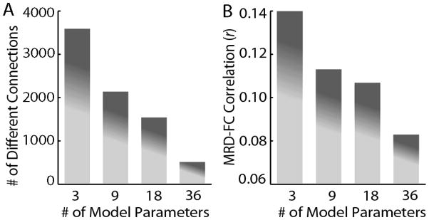
Connectivity-based outcome measures from confound regression models using whole-brain motion parameters. Higher-order confound regression models result in fewer significantly different (FDR Q<0.05) connections between the high and low motion groups (A) and a diminished mean absolute correlation between subject MRD and pairwise connectivity (B).

Similarly, the better model fit of higher-parameter models was indicated by lower AIC values (Figure 6B). The 36-parameter model had the lowest average AIC value. The delta-AIC between the 36-parameter model and all other lower-parameter models was significant, with a delta-AIC of 4 versus the 18-parameter model, a delta-AIC of 7 versus the 9-parameter model, and a delta-AIC of 42 versus the 3- parameter model. However, this was largely driven by the high-motion group: AIC values declined for the low motion group when six standard motion parameters were included, but the AIC in this group did not drop when derivative and quadratic terms were added in the 18- and 36-parameter models. In contrast, in the high-motion group AIC values continued to decline at each step as more parameters were added.

Paralleling the results of these regression diagnostic measures, connectivity-based outcomes improved with high-parameter confound regression models (Figure 7). Notably, the 36-parameter model had the lowest number of significantly different connections between the high and low motion groups (Figure 7A). In addition, the 36-parameter model had the lowest mean absolute correlation between connectivity and motion (Figure 7B). Pairwise comparisons between the 36-parameter model and all other models were highly statistically significant; when the 36-parameter model was compared to the 18-parameter model (which was next-best), the 36 parameter model showed less connections that were different between the high and low motion groups (z=46.09; p<1.0×10⁻¹⁰) and a lower correlation between motion and connectivity (z=62.60; p<1.0×10⁻¹⁰)

Confound regression using voxelwise motion parameters

Since motion was highly correlated across the entire brain, we did not expect that voxelwise motion parameters would provide substantial superiority over whole-brain motion parameters. As seen in Supplementary Figure 4, the 24-parameter regression model based on voxelwise parameters was slightly inferior to the 36-parameter whole-brain confound regression model on all outcome measures. The delta-AIC between the two models was 5.6; the 36-parameter whole brain model also had a smaller difference between high and low motion groups (z=13.75; p<1.0×10⁻¹⁰) and a lower correlation between connectivity and motion (z=44.20; p<1.0×10⁻¹⁰).

Control analyses

To address the concern that high-parameter models might remove real brain signal along with motion-induced noise, we conducted a control analysis examining the influence of increased number of confound regressors on distant connections in low motion subjects. We did not find any evidence for diminished connectivity across the 9-, 18-, and 36-parameter models (r=0.25–0.26 for all models). As expected, addition of random noise regressors did not alter model adjusted r² (Figure 8A), and worsened (increased) model AIC (Figure 8C). In contrast, connectivity-based outcome measures were driven by the addition of noise regressors, diminishing differences between the high and low motion groups (Figure 8B) and reducing the overall correlation between motion and connectivity (Figure 4D). This suggests that when evaluating confound regression techniques, connectivity-based outcome measures should not be considered in isolation, but always evaluated in tandem with regression diagnostics (such as adjusted r² and AIC) that consider model fit within the context of degrees of freedom.

Figure 8.

Control analysis investigating the effect of including increasing numbers of noise regressors on regression diagnostic outcomes and connectivity-based outcome measures. Whole-brain confound regression models are shown in black. The grey line plot indicates confound regression models that included a variable number of noise regressors. All noise regression models consist of 3 confound regressors that were constructed from real data (global signal, white matter, CSF), plus a variable number (6, 15, 33) of randomly generated noise regressors. Adding noise regressors does not increase the variance explained by the model as measured by the adjusted r² (A). Addition of noise regressors worsens model fit as measured by AIC (C). However, adding noise regressors does modestly reduce the # of different connections between matched high and low motion groups (B) and the mean absolute correlation between subject MRD and pairwise functional connectivity (D). However, these effects are much smaller than the gains observed by including real motion parameters (black line).

Confound regression of motion spikes

Next, we investigated if adding more confound regressors corresponding to motion spikes could further improve performance. Regression diagnostics (AIC and adjusted r²) were calculated for each spike regression model, which also included as a base 36 whole brain motion parameters as detailed above. Both the single criterion (relative RMS displacement) and the dual-criteria (relative RMS + DVARS) approaches produced a mean adjusted r² of 0.65 across all temporal windows. However, the mean AIC of the single criterion was lower than the AIC of the dual criteria method across all temporal windows; the mean single criterion AIC was 1222, whereas the dual criteria AIC was 1235 (delta-AIC=13). The AIC of the single-criterion (but not dual-criteria) spike regression compared favorably to that of the 36-parameter model alone (AIC=1231; delta-AIC=9).

When different spike identification techniques and windows were evaluated using connectivity based outcome measures, all spike-regression methods produced a substantial improvement over confound regression with the 36-parameter model alone (Figure 9). Furthermore, there was evidence for the improvement with the single-criterion relative RMS displacement approach. In particular, regression of spikes without a temporal window (i.e., only at the timepoint immediately following motion) from spikes identified using the single-criterion method produced the least number of significantly different connections between the high and low motion groups (Figure 9A) and the lowest mean absolute correlation between connectivity and motion (Figure 9B). The difference between single-criterion, single-TR spike regression was statistically significant when compared to the next best model for both difference between high and low motion groups (comparator model: single-criterion, 1b,0f; z=8.00, p<1.0×10⁻¹⁰) as well as the correlation between motion and connectivity (comparator model: single-criterion 0b,1f; z=8.47, p<1.0×10⁻¹⁰). As expected, among subjects who had spikes identified, the adjusted r² values were higher in those with more spikes (Figure 9C).

Figure 9.

Confound regression of motion spikes. Spike regression was evaluated using a single-criterion identification method (relative RMS displacement; grey diamonds) and a dual-criteria method (relative RMS displacement + DVARS; black circles). These two methods were tested over a range of windows (xb,yf denotes x TRs before spike, y TRs after spike). The single-criterion approach without an expanded temporal window (0b,0f) produced the least number of significantly different connections between high and low motion groups (A) and the lowest mean absolute correlation between MRD and functional connectivity (B). Variance explained by single-criterion spike regression model without a window (among subjects where spikes were identified) was highly related to the number of spikes present for a given subject (C).

Band-pass filtering

Previous analyses of unregressed magnitude spectra indicated that motion increased signal magnitude across both low and high frequencies. However, bandpass filtering in our framework occurs after confound regression; therefore, we reevaluated the effects of motion on the magnitude spectra following confound regression. As displayed in Figure 10, confound regression dramatically altered the spectral characteristics of the motion confound. Differences between high and low motion groups were present at all frequencies for the 3- and 9-paramter models. This was also the case for the 18-parameter model, except at 0.0389 Hz (where a trend was present). In the 36-parameter model, groups were significantly different at all frequencies above 0.0139 Hz except isolated frequencies including 0.0278, 0.0306, 0.0389, and 0.0528 Hz. In contrast to such generally global differences, when the improved (36-parameter + spike regression) confound regression model was applied, significant differences between the high and low motion groups were only seen at frequencies at or above 0.08 Hz.

Figure 10.

Effects of confound regression on magnitude spectra of rsfc-MRI data. A) Confound regression progressively diminishes the generalized effect of greater magnitude for the high motion group. B) When improved confound regression (36 parameters + spike regression) is applied, high and low motion groups diverge only at frequencies above 0.08 Hz. Starred grey bar indicates a significant difference between magnitude of high and low motion groups at each frequency.

Based on this information, we compared band-pass filtering using a 0.01–0.1 Hz filter to a filter retaining frequencies between 0.01–0.08Hz. Regression procedures were the same for both, utilizing the improved 36-parameter + single criterion, single-TR (0b,0f) spike regression. Filtering at 0.01–0.08Hz reduced the number of different connections between the high and low motion groups (86 versus 154 connections); this difference was statistically significant (z=20.68, p<1.0×10⁻¹⁰). Additionally, the 0.01–0.08 Hz bandpass filter produced a statistically significant reduction in the mean absolute correlation between connectivity and motion (r=0.065 versus r=0.068; z=13.29, p<1.0×10⁻¹⁰).

Effect of improved preprocessing on network modularity

As a final evaluation of the benefits of improved preprocessing, we compared the community structure of the whole-brain networks in high and low motion groups under standard and improved preprocessing using normalized mutual information (Power et al. 2011). Community structure for all four conditions is described in Supplementary Table 2. As seen in Figure 11, the community structure in the low motion group was nearly identical under both preprocessing streams (NMI=0.96). In contrast, the community structure of the high motion group was substantially altered by improved preprocessing (NMI=0.73). This shift was in part the result of the community structure of the high-motion group becoming more similar to that of the low motion group. Under standard preprocessing, low and high motion groups were fairly dissimilar in terms of community structure (NMI 0.70). In contrast, when the low and high motion groups were compared following improved preprocessing, NMI was 0.86. This NMI value was statistically significant (p=0.003) when compared to a null distribution of 1000 NMI values resulting from community structures of average networks produced by randomly permuted (standard versus improved) preprocessing.

Figure 11.

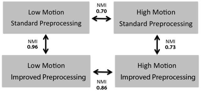
Improved preprocessing reduces differences in community structure between low and high motion groups. The community structure of low-motion subjects is extremely similar under both standard and improved preprocessing. However, with improved preprocessing the community structure of the high-motion group’s network becomes much more similar to that of the low motion group than when using standard preprocessing procedures.

Number of volumes flagged for scrubbing after improved preprocessing

Lastly, we compared the number of volumes flagged for scrubbing following standard and improved preprocessing as described above. Using standard preprocessing, 72 subjects had volumes flagged for scrubbing (mean # of volumes scrubbed per subject: 0.88; S.D. 2.64); of these subjects, 8 would have <4 minutes of data after scrubbing. In contrast, following improved preprocessing, we found that only 3 subjects of 348 had volumes flagged for scrubbing (mean 0.029 volumes; S.D. 0.3934); none would have <4 minutes of data. The difference in number of volumes flagged for scrubbing was significantly different between the two pipelines (z=7.41, p<1.0×10⁻¹⁰).

DISCUSSION

Motion artifact is a primary obstacle impeding the application of rsfc-MRI to the study of individual and group differences. Therefore, understanding and mitigating the influence of this artifact is critical. Our results further describe the spatial, temporal, and spectral characteristics of motion artifact in rsfc-MRI data, providing information that can guide efforts to minimize its effect. Systematic analyses indicate that improved confound regression and filtering can substantially attenuate—though not eliminate—motion artifact. A summary of the proposed improved pipeline and important considerations at each step in the process is presented in Figure 12.

Figure 12.

Summary of recommended preprocessing pipeline and critical considerations. We emphasize that this pipeline is not prescriptive, will likely be subject to rapid evolution, and should be tailored to individual study goals and datasets.

Characteristics of motion artifact

In order to better account for motion artifact in rsfc-MRI data, it is important to understand its properties. Our analyses indicate that motion artifact is relatively spatially distributed, temporally constrained, and frequency-nonspecific. Voxelwise analyses of motion-related displacement suggest that, while there is some heterogeneity in motion-induced displacement, in general the displacement of voxels is highly correlated across the brain. As a result, the effects of motion tend to be spatially distributed: motion causes a substantial drop in signal intensity across the entire brain parenchyma. Notably, the opposite occurs around the rim of the brain where motion results in large increases in BOLD signal.

Additionally, the drop in signal intensity associated with motion appears to be temporally constrained, mainly affecting the two timepoints around which motion occurs. As noted by Power et al. (2011), the effect of motion seems to scale with the amplitude of the displacement: greater amplitude displacements are associated with greater change in BOLD signal. As discussed below, this is an important topic that merits further attention, as it impacts the way in which motion “spikes” are defined for regression, scrubbing, or de-weighting.

Finally, the effect of motion does not appear to reside uniquely in one frequency domain; motion tends to increase signal magnitude across the frequency spectrum in rsfc-MRI data. Mapping the spectral characteristics of motion artifact is important as it impacts the optimal design of the filter to be applied. Had motion only caused high frequency artifact, the judicious application of a well-designed band-pass filter could completely remove it, obviating the need for confound regression. However, this is not the case: confound regression is critical for removing artifact, and in the process further isolates the frequencies at which motion artifact is apparent, increasing the utility of subsequent temporal filtering.

Global signal regression biases the apparent structure of motion artifact

The initial three reports on motion artifact in rsfc-MRI data (Power et al., 2011; Satterthwaite et al., 2012; Van Dijk et al., 2011) emphasized the degree to which motion artifact is modulated by the distance between connections. All three studies documented that increased subject motion is associated with increased connectivity between nodes that are relatively close together, but simultaneously associated with diminished connectivity between more distant nodes. Here, by analyzing both real and simulated data, we establish that this pattern of motion artifact is largely determined by the inclusion of the global signal in confound regression: when the global signal (or similar mean WM or CSF signals) are not included in confound regression, the effect of motion is simply to increase connectivity. This effect is still most prominent at nodes that are close together, and decays somewhat with greater distance. As illustrated by analyses of voxelwise motion parameters (Figure 2), this distance-dependent decay is the result of the fact that displacement and resulting artifact at nodes that are far apart are less highly correlated. It should be noted that this effect was previously shown (but not emphasized) by Power et al. (2011); see their Figure 9. We believe that the predominant effect of motion, typically produced by z-axis displacement (e.g., nodding) that shifts tissue perpendicular to the excitation slice plane, is to introduce widely distributed and often very large reductions in BOLD signal. This global artifact diffusely increases simple timeseries correlations, but its consistent timing and valence across the brain allows it to be removed effectively by covarying for the global brain timeseries. However, motion also introduces artifacts that have the same valence in nearby regions but opposite (anticorrelated) valence in regions distant from each other (Power et al. 2011). These regionally heterogeneous effects are unmasked by inclusion of a global covariate and explain the local vs. distal effects previously reported (see Supplementary Material for detailed analysis and discussion of this effect). Given the debate regarding the merits of including global signal in rsfc-MRI preprocessing (Murphy et al., 2009; Fox et al., 2009; Weissenbacher et al., 2009), and since not all studies include the global signal in confound regression, the presence of motion artifact and its effects on connectivity should be evaluated within the context of the preprocessing scheme used.

High-parameter confound regression models are potentially beneficial

We developed an improved preprocessing pipeline for rsfc-MRI data that is more robust to the influences of motion artifact. We found that improved preprocessing can produce substantial advantages relative to standard preprocessing measures, and greatly attenuate—but not completely remove—motion artifacts in rsfc-MRI data. Initially, we examined confound regression models with expanded numbers of whole-brain motion parameters, which sequentially included temporal derivative and quadratic terms (Friston et al., 1996; Zu Eulenburg, 2012). There was clear evidence for the relative benefit of higher-parameter models, with the 36-parameter model showing the best performance across both regression-diagnostic and connectivity-based outcome measures.

Importantly, with this regression procedure we did not see any evidence for removal of real brain signal along with noise (Ollinger et al., 2009) among the long-distance connections that are likely to be particularly susceptible to such effects. Furthermore, control analyses with noise regressors could not explain the observed pattern of results: while connectivity-based outcome measures may respond nonspecifically to increased numbers of regressors, regression diagnostic measures worsen as nonspecific noise regressors are added to the model. However, it is important to note that high-parameter models seem to primarily benefit subjects with greater levels of motion, as evinced by the flat AIC values in the low-motion group for the 18- and 36-parameter models, as well as the clear relationship between variance explained (adjusted r²) and subject MRD. These results suggest that the optimal confound regression strategy will vary by study and subject population: studies with nearly motionless subjects (i.e., healthy undergraduates) may not benefit from a high-parameter approach, whereas datasets with greater degrees of motion (i.e., youth or clinical samples) are likely to preferentially benefit from a higher-parameter confound regression model.

Spike regression censors motion artifact at individual TRs

As suggested previously (Lemieux et al., 2007), we found that the addition of spike regressors provided a substantial benefit over use of 36-parameter confound regression model alone. It is likely that spike regression provides this benefit because the relationship between motion and the BOLD signal may be neither linear nor quadratic with higher degrees of movement (Lemieux et al., 2007). Similarly, while the average timecourse of motion artifact is relatively constrained to the two timepoints bounding a movement, for each individual movement there is likely a great deal of heterogeneity in the effect on BOLD signal. The fact that the BOLD signal change created by a motion spike is in fact unlikely to be consistently shaped like a boxcar or any other fixed shape is the reason that expanding the temporal window around a given motion spike was not found to be helpful during spike regression. Thus, any temporal window that models motion-related effects using a fixed shape will suffer from poor fit. In contrast, a single regressor for a spike at a given timepoint effectively removes the influence of that timepoint from subsequent correlation analysis of the resulting residual data. Though implemented differently, our approach of including spike regressors is extremely similar in the final result to the updated scrubbing procedure outlined by Power et al. (2012). This accounts for the fact that very few volumes were flagged for scrubbing as a second stage in addition to spike regression following improved preprocessing.

One difference from the method of Power et al. (2012) is their use of a censoring of a wider temporal window (i.e., 1 timepoint point before and 2 timepoints after) a motion-induced spike. This could be implemented using spike regression as well, but it would be necessary to model each TR of the window separately as its own regressor. We did not pursue such an approach as it quickly led to an unreasonably large number of spike confound regressors (i.e., >40) in higher-motion subjects, leading to their exclusion due to insufficient (i.e., <4 minutes) of data remaining. A lower threshold for spike identification similarly excluded more subjects due to insufficient data. It should be emphasized that this data quality versus data quantity tradeoff is of particular concern in studies of subjects who are movement-prone (children, patients) with brief resting-state acquisitions. Studies of healthy undergraduates or those with longer acquisition durations may be able to lower the spike threshold or assign multiple regressors for each spike without compromising the remaining timeseries duration. One potential solution to the problem of thresholding spike regression is the use of a variance-weighting approach that de-weights timepoints along a continuum on the basis of signal quality and the presence of detected artifact (Diedrichsen and Shadmehr, 2005). Although not yet applied to rsfc-MRI data, such an approach could integrate the virtues of a spike-regression approach but without the need to select an arbitrary threshold for designating the presence of a spike.

Tailoring band-pass filtering improves control of motion

Following improved confound regression we found that the magnitude spectra of high and low motion subjects diverged only at relatively high frequencies (>0.08Hz). Notably, the frequencies impacted by artifact vary according to the confound regression applied. Accordingly, selection of the optimal filter may depend on which confound regression approach was pursued, as well as acquisition-related data characteristics. In this study, we found that a filter with a low-pass cutoff of 0.08 Hz performed better than a low-pass filter of 0.1 Hz. However, it should be noted that these “improved” filter settings are in fact quite similar to those routinely used in prior work (Power et al., 2011; Van Dijk et al., 2011). We caution that removal of higher-frequency signals through band-filtering may remove signal that contributes to resting state networks (Niazy et al., 2011). However, our analyses indicate that higher frequency signals are more likely to be related to differences in subject motion even following improved confound regression; the removal of these frequencies may therefore improve the ability to detect group and individual differences that are not related to motion. Finally, we note that most rsfc-MRI studies do not report the characteristics of the band-pass filter used; given concern regarding filter-induced ringing artifacts in the data (Carp, 2012; Power et al., 2012) we encourage future studies to provide details regarding filter design (such as filter order).

Future Directions and Limitations

There are several limitations to the current work that should be acknowledged. First and most importantly, in this study we used 4 surrogate outcome measures in the context of not knowing the ground truth of what is signal and what is noise in rsfc-MRI data. By examining measures such as AIC that privilege parsimony, we aimed to strike a balance between the competing goals of maximally removing noise without removing brain signal. However, it should be emphasized that such measures provide only an indirect measure of effectiveness, as they only report the degree to which a given confound regression procedure fits the data. In order to provide convergent evidence, we also employed connectivity-based outcome measures. However, our control analyses indicate that “improvement” on these measures can be driven simply by adding greater numbers of random regressors to the confound regression model, underlining their limited utility as an outcome measure when evaluated in isolation. In contrast to the connectivity-based outcome measures, the adjusted r² and AIC values were not improved by the addition of random confound regressors, suggesting that the regression-based and connectivity-based outcome measures should be evaluated together. Thus, the outcome measures used in the present study are not definitive, and future research will benefit from experimental designs dedicated to the investigation of this issue. Specifically, in future work we hope to implement a within-subject design where connectivity is assessed in motionless subjects and then compared to connectivity in subjects where small amounts of motion artifact are added to the acquisition in a controlled fashion. Such an experiment would allow us to better separate signal from noise in rsfc-MRI data.

Second, in this study we assume that any differences between the matched high and low motion group are attributable to motion itself. However, in the current across-subjects study design we cannot completely exclude the possibility that observed differences related to motion are due not just to motion alone but also to subject factors that were not controlled for during the matching process.

Third, there are several important approaches to artifact removal that we did not evaluate, most notably independent components analysis (Tohka et al., 2008; Churchill et al., 2012b). Such approaches should be evaluated fully in future studies and compared to the confound regression strategies outlined here. In particular, approaches such as fully exploratory network ICA (FENICA; Schöpf et al., 2010; Schöpf et al., 2011) and CompCor (Behzadi et al. 2007; Chai et al. 2011) may help gain traction towards this goal in the future.

Fourth, as noted above, our approach presupposes the use of a standard pipeline across all subjects. One potentially attractive alternative to choosing such a rigid processing pipeline is the use of subject-specific processing pipelines. While they have yet to be validated in rsfc-MRI data, advanced tools exist that would allow heterogeneous samples to receive tailored preprocessing in a data-driven manner (Zhang et al., 2009; Strother et al., 2002; Churchill et al., 2012a). It will be of great interest to ascertain whether such tools can be adapted towards specific use in rsfc-MRI data, and scaled to accommodate very large imaging-genomic datasets.

Fifth, a potentially important issue not addressed in the current work is the statistical implications of the practice of extracting connectivity measures in the form of correlations from the residual timeseries data following confound regression. One consequence of this standard practice is the loss of information regarding degrees of freedom: the connectivity measure obtained from the residual data does not consider nor penalize the number of regressors used during confound regression. This may be of particular concern when subjects have timeseries of different initial length, the timeseries are shortened via scrubbing to disparate durations, or divergent numbers of regressors are used during confound regression. This effect is not likely to be substantial for short timeseries acquisitions where the amount of data lost to scrubbing is limited by requirements that a minimum amount of real data remains after scrubbing or spike regression (in this case, 4 minutes). In the present dataset, the statistical significance of correlation values calculated from 80 timepoints (the floor) or 120 timepoints (the maximum) are quite similar. However, with a very long acquisition timeseries a situation could arise where a high proportion of data might be removed by scrubbing, producing cases where a subject with 5 minutes of data was being compared to another subject with 1 hour of data. In such cases, it seems likely that the current standard of calculating Pearson’s correlations from residual timeseries would need to be modified. Options include corrections for degrees of freedom (such as the Bartlett correction, see Van Dijk et al., 2010) or alternate approaches such as such as calculating connectivity through regressions where scrubbing or despiking is performed simultaneously, thus allowing information regarding signal variance and degrees of freedom to be retained. Furthermore, such regressions could integrate autocorrelation correction procedures (as implemented in neuroimaging packages such as FSL; Woolrich et al., 2009), which account for the lack of temporal independence in fMRI timeseries data that violate the assumptions of Pearson’s correlations. Additionally, an alternative utilizing generalized estimated equations that account for temporal dependence (D’Angelo et al., 2011) has recently been proposed and may merit wider application.

Sixth, while we did not find a benefit for the use of voxelwise displacement parameters in confound regression, this does not preclude their potential effectiveness in general. For example, voxelwise displacement parameters may be beneficial for analyses of connections between specific nodes where displacements are particularly divergent and thus poorly captured by whole-brain motion parameters. Additionally, it is possible that externally-recorded motion tracking (Tremblay et al., 2005) may provide superior performance and better estimation of voxelwise displacement.

Seventh, while we focused on the effects of in-scanner head motion on functional connectivity, physiologic signals such as heart and respiration rate also have a substantial influence on rsfc-MRI data (Auer, 2008; Birn et al., 2006; Chang and Glover, 2009; Shmueli et al., 2007). Methods exist for the control of such signals, and should be considered alongside methods to reduce the influence of motion artifact in rsfc-MRI data (Jones et al., 2008; Glover et al., 2000; Churchill et al., 2012a).

Eighth and finally, as fast TR acquisitions become more common (Feinberg et al., 2010), slice timing correction may be avoided, perhaps allowing the effects of motion to be better isolated to the volumes in which motion occurs.

Conclusion and Summary

The present results suggest that, when compared to standard techniques, improved preprocessing can substantially reduce the burden of artifact induced by in-scanner head motion in rsfc-MRI data. However, it should be emphasized that the procedures examined herein do not result in the elimination of motion artifact, and that the residual effects of motion are still substantial enough to represent an important confound to rsfc-MRI studies of individual difference and psychopathology, especially in developmental populations (Church et al., 2010; Luna et al., 2010). Therefore, we continue to recommend that subject motion be explicitly reported as an important outcome measure in all rsfc-MRI studies. We also suggest that, regardless of the preprocessing techniques applied, motion should be matched with respect to the outcome of interest. Nonetheless, improved preprocessing techniques that mitigate the influence of motion artifact remain of value, as reducing the noise in rsfc-MRI should inevitably increase sensitivity to detect real differences in connectivity and network structure among individuals and groups (Guo et al., 2012).

Highlights.

• We describe spatial, temporal, and spectral features of rsfc-MRI motion artifact.

• We show how these artifact features impact preprocessing choices.

• We systematically evaluate different confound regression and filtering techniques.

• Our optimized preprocessing approach minimizes rsfc-MRI motion artifact.

References

- Akaike H. A new look at the statistical model identification. Automatic Control, IEEE Transactions on. 1974;19:716–723. [Google Scholar]
- Auer DP. Spontaneous low-frequency blood oxygenation level-dependent fluctuations and functional connectivity analysis of the ‘resting’ brain. Magn Reson Imaging. 2008;26:1055–1064. doi: 10.1016/j.mri.2008.05.008. [DOI] [PubMed] [Google Scholar]
- Bassett DS, Bullmore E, Verchinski BA, Mattay VS, Weinberger DR, Meyer-Lindenberg A. Hierarchical organization of human cortical networks in health and schizophrenia. J Neurosci. 2008;28:9239–9248. doi: 10.1523/JNEUROSCI.1929-08.2008. [DOI] [PMC free article] [PubMed] [Google Scholar]
- Behzadi Y, Restom K, Liau J, Liu TT. A component based noise correction method (CompCor) for BOLD and perfusion based fMRI. Neuroimage. 2007;37:90–101. doi: 10.1016/j.neuroimage.2007.04.042. [DOI] [PMC free article] [PubMed] [Google Scholar]
- Birn RM, Diamond JB, Smith MA, Bandettini PA. Separating respiratory-variation-related fluctuations from neuronal-activity-related fluctuations in fMRI. Neuroimage. 2006;31:1536–1548. doi: 10.1016/j.neuroimage.2006.02.048. [DOI] [PubMed] [Google Scholar]
- Biswal B, Yetkin FZ, Haughton VM, Hyde JS. Functional connectivity in the motor cortex of resting human brain using echo-planar MRI. Magn Reson Med. 1995;34:537–541. doi: 10.1002/mrm.1910340409. [DOI] [PubMed] [Google Scholar]
- Biswal BB, Mennes M, Zuo XN, Gohel S, Kelly C, Smith SM, Beckmann CF, Adelstein JS, Buckner RL, Colcombe S, Dogonowski AM, Ernst M, Fair D, Hampson M, Hoptman MJ, Hyde JS, Kiviniemi VJ, Kötter R, Li SJ, Lin CP, Lowe MJ, Mackay C, Madden DJ, Madsen KH, Margulies DS, Mayberg HS, McMahon K, Monk CS, Mostofsky SH, Nagel BJ, Pekar JJ, Peltier SJ, Petersen SE, Riedl V, Rombouts SA, Rypma B, Schlaggar BL, Schmidt S, Seidler RD, Siegle GJ, Sorg C, Teng GJ, Veijola J, Villringer A, Walter M, Wang L, Weng XC, Whitfield-Gabrieli S, Williamson P, Windischberger C, Zang YF, Zhang HY, Castellanos FX, Milham MP. Toward discovery science of human brain function. Proc Natl Acad Sci U S A. 2010;107:4734–4739. doi: 10.1073/pnas.0911855107. [DOI] [PMC free article] [PubMed] [Google Scholar]
- Bullmore ET, Brammer MJ, Rabe-Hesketh S, Curtis VA, Morris RG, Williams SC, Sharma T, McGuire PK. Methods for diagnosis and treatment of stimulus-correlated motion in generic brain activation studies using fMRI. Hum Brain Mapp. 1999;7:38–48. doi: 10.1002/(SICI)1097-0193(1999)7:1<38::AID-HBM4>3.0.CO;2-Q. [DOI] [PMC free article] [PubMed] [Google Scholar]
- Buckner RL, Krienen FM, Castellanos A, Diaz JC, Yeo BT. The organization of the human cerebellum estimated by intrinsic functional connectivity. J Neurophysiol. 2011;106:2322–2345. doi: 10.1152/jn.00339.2011. [DOI] [PMC free article] [PubMed] [Google Scholar]
- Carp J. Optimizing the order of operations for movement scrubbing: Comment on Power et al. Neuroimage. 2011 doi: 10.1016/j.neuroimage.2011.12.061. [DOI] [PubMed] [Google Scholar]
- Chai XJ, Castañón AN, Ongür D, Whitfield-Gabrieli S. Anticorrelations in resting state networks without global signal regression. Neuroimage. 2012;59:1420–1428. doi: 10.1016/j.neuroimage.2011.08.048. [DOI] [PMC free article] [PubMed] [Google Scholar]
- Chang C, Glover GH. Effects of model-based physiological noise correction on default mode network anti-correlations and correlations. Neuroimage. 2009;47:1448–1459. doi: 10.1016/j.neuroimage.2009.05.012. [DOI] [PMC free article] [PubMed] [Google Scholar]
- Church JA, Petersen SE, Schlaggar BL. The “Task B problem” and other considerations in developmental functional neuroimaging. Hum Brain Mapp. 2010;31:852–862. doi: 10.1002/hbm.21036. [DOI] [PMC free article] [PubMed] [Google Scholar]
- Churchill NW, Oder A, Abdi H, Tam F, Lee W, Thomas C, Ween JE, Graham SJ, Strother SC. Optimizing preprocessing and analysis pipelines for single-subject fMRI. I. Standard temporal motion and physiological noise correction methods. Hum Brain Mapp. 2012a;33:609–627. doi: 10.1002/hbm.21238. [DOI] [PMC free article] [PubMed] [Google Scholar]
- Churchill NW, Yourganov G, Oder A, Tam F, Graham SJ, Strother SC. Optimizing Preprocessing and Analysis Pipelines for Single-Subject fMRI: 2. Interactions with ICA, PCA, Task Contrast and Inter-Subject Heterogeneity. PLoS One. 2012b;7:e31147. doi: 10.1371/journal.pone.0031147. [DOI] [PMC free article] [PubMed] [Google Scholar]
- Cordes D, Haughton VM, Arfanakis K, Carew JD, Turski PA, Moritz CH, Quigley MA, Meyerand ME. Frequencies contributing to functional connectivity in the cerebral cortex in “resting-state” data. AJNR Am J Neuroradiol. 2001;22:1326–1333. [PMC free article] [PubMed] [Google Scholar]
- D’Angelo GM, Lazar NA, Eddy WF, Morris JC, Sheline YI. A generalized estimating equations approach for resting-state functional MRI group analysis. Conf Proc IEEE Eng Med Biol Soc. 2011;2011:5064–5067. doi: 10.1109/IEMBS.2011.6091254. [DOI] [PMC free article] [PubMed] [Google Scholar]
- Diedrichsen J, Shadmehr R. Detecting and adjusting for artifacts in fMRI time series data. Neuroimage. 2005;27:624–634. doi: 10.1016/j.neuroimage.2005.04.039. [DOI] [PMC free article] [PubMed] [Google Scholar]
- Dosenbach NU, Nardos B, Cohen AL, Fair DA, Power JD, Church JA, Nelson SM, Wig GS, Vogel AC, Lessov-Schlaggar CN, Barnes KA, Dubis JW, Feczko E, Coalson RS, Pruett JR, Barch DM, Petersen SE, Schlaggar BL. Prediction of individual brain maturity using fMRI. Science. 2010;329:1358–1361. doi: 10.1126/science.1194144. [DOI] [PMC free article] [PubMed] [Google Scholar]
- Feinberg DA, Moeller S, Smith SM, Auerbach E, Ramanna S, Gunther M, Glasser MF, Miller KL, Ugurbil K, Yacoub E. Multiplexed echo planar imaging for sub-second whole brain FMRI and fast diffusion imaging. PLoS One. 2010;5:e15710. doi: 10.1371/journal.pone.0015710. [DOI] [PMC free article] [PubMed] [Google Scholar]
- Fox MD, Snyder AZ, Vincent JL, Corbetta M, Van Essen DC, Raichle ME. The human brain is intrinsically organized into dynamic, anticorrelated functional networks. Proc Natl Acad Sci U S A. 2005;102:9673–9678. doi: 10.1073/pnas.0504136102. [DOI] [PMC free article] [PubMed] [Google Scholar]
- Fox MD, Raichle ME. Spontaneous fluctuations in brain activity observed with functional magnetic resonance imaging. Nat Rev Neurosci. 2007;8:700–711. doi: 10.1038/nrn2201. [DOI] [PubMed] [Google Scholar]
- Fox MD, Zhang D, Snyder AZ, Raichle ME. The global signal and observed anticorrelated resting state brain networks. J Neurophysiol. 2009;101:3270–3283. doi: 10.1152/jn.90777.2008. [DOI] [PMC free article] [PubMed] [Google Scholar]
- Fox MD, Greicius M. Clinical applications of resting state functional connectivity. Front Syst Neurosci. 2010;4:19. doi: 10.3389/fnsys.2010.00019. [DOI] [PMC free article] [PubMed] [Google Scholar]
- Friston KJ, Williams S, Howard R, Frackowiak RS, Turner R. Movement-related effects in fMRI time-series. Magn Reson Med. 1996;35:346–355. doi: 10.1002/mrm.1910350312. [DOI] [PubMed] [Google Scholar]
- Glahn DC, Winkler AM, Kochunov P, Almasy L, Duggirala R, Carless MA, Curran JC, Olvera RL, Laird AR, Smith SM, Beckmann CF, Fox PT, Blangero J. Genetic control over the resting brain. Proc Natl Acad Sci U S A. 2010;107:1223–1228. doi: 10.1073/pnas.0909969107. [DOI] [PMC free article] [PubMed] [Google Scholar]
- Glover GH, Li TQ, Ress D. Image-based method for retrospective correction of physiological motion effects in fMRI: RETROICOR. Magn Reson Med. 2000;44:162–167. doi: 10.1002/1522-2594(200007)44:1<162::aid-mrm23>3.0.co;2-e. [DOI] [PubMed] [Google Scholar]
- Guo CC, Kurth F, Zhou J, Mayer EA, Eickhoff SB, Kramer JH, Seeley WW. One-year test-retest reliability of intrinsic connectivity network fMRI in older adults. NeuroImage. 2012 doi: 10.1016/j.neuroimage.2012.03.027. [DOI] [PMC free article] [PubMed] [Google Scholar]
- Gur RC, Richard J, Calkins ME, Chiavacci R, Hansen JA, Bilker WB, Loughead J, Connolly JJ, Qiu H, Mentch FD, Abou-Sleiman PM, Hakonarson H, Gur RE. Age group and sex differences in performance on a computerized neurocognitive battery in children age 8–21. Neuropsychology. 2012;26:251–265. doi: 10.1037/a0026712. [DOI] [PMC free article] [PubMed] [Google Scholar]
- Hopfinger JB, Büchel C, Holmes AP, Friston KJ. A study of analysis parameters that influence the sensitivity of event-related fMRI analyses. Neuroimage. 2000;11:326–333. doi: 10.1006/nimg.2000.0549. [DOI] [PubMed] [Google Scholar]
- Jenkinson M, Bannister P, Brady M, Smith S. Improved optimization for the robust and accurate linear registration and motion correction of brain images. Neuroimage. 2002;17:825–841. doi: 10.1016/s1053-8119(02)91132-8. [DOI] [PubMed] [Google Scholar]
- Johnstone T, Ores Walsh KS, Greischar LL, Alexander AL, Fox AS, Davidson RJ, Oakes TR. Motion correction and the use of motion covariates in multiple-subject fMRI analysis. Hum Brain Mapp. 2006;27:779–788. doi: 10.1002/hbm.20219. [DOI] [PMC free article] [PubMed] [Google Scholar]
- Jones TB, Bandettini PA, Birn RM. Integration of motion correction and physiological noise regression in fMRI. Neuroimage. 2008;42:582–590. doi: 10.1016/j.neuroimage.2008.05.019. [DOI] [PMC free article] [PubMed] [Google Scholar]
- Lemieux L, Salek-Haddadi A, Lund TE, Laufs H, Carmichael D. Modelling large motion events in fMRI studies of patients with epilepsy. Magn Reson Imaging. 2007;25:894–901. doi: 10.1016/j.mri.2007.03.009. [DOI] [PubMed] [Google Scholar]
- Luna B, Velanova K, Geier CF. Methodological approaches in developmental neuroimaging studies. Hum Brain Mapp. 2010;31:863–871. doi: 10.1002/hbm.21073. [DOI] [PMC free article] [PubMed] [Google Scholar]
- Murphy K, Birn RM, Handwerker DA, Jones TB, Bandettini PA. The impact of global signal regression on resting state correlations: are anti-correlated networks introduced? Neuroimage. 2009;44:893–905. doi: 10.1016/j.neuroimage.2008.09.036. [DOI] [PMC free article] [PubMed] [Google Scholar]
- Niazy RK, Xie J, Miller K, Beckmann CF, Smith SM. Spectral characteristics of resting state networks. Prog Brain Res. 2011;193:259–276. doi: 10.1016/B978-0-444-53839-0.00017-X. [DOI] [PubMed] [Google Scholar]
- Ollinger JM, Oakes TR, Alexander AL, Haeberli F, Dalton KM, Davidson RJ. The secret life of motion covariates. Neuroimage. 2009;47:122. [Google Scholar]
- Power JD, Barnes KA, Snyder AZ, Schlaggar BL, Petersen SE. Spurious but systematic correlations in functional connectivity MRI networks arise from subject motion. Neuroimage. 2011 doi: 10.1016/j.neuroimage.2011.10.018. [DOI] [PMC free article] [PubMed] [Google Scholar]
- Power JD, Cohen AL, Nelson SM, Wig GS, Barnes KA, Church JA, Vogel AC, Laumann TO, Miezin FM, Schlaggar BL, Petersen SE. Functional network organization of the human brain. Neuron. 2011;72:665–678. doi: 10.1016/j.neuron.2011.09.006. [DOI] [PMC free article] [PubMed] [Google Scholar]
- Rubinov M, Sporns O. Complex network measures of brain connectivity: uses and interpretations. Neuroimage. 2010;52:1059–1069. doi: 10.1016/j.neuroimage.2009.10.003. [DOI] [PubMed] [Google Scholar]
- Rubinov M, Sporns O. Weight-conserving characterization of complex functional brain networks. Neuroimage. 2011;56:2068–2079. doi: 10.1016/j.neuroimage.2011.03.069. [DOI] [PubMed] [Google Scholar]
- Satterthwaite TD, Wolf DH, Loughead J, Ruparel K, Elliott MA, Hakonarson H, Gur RC, Gur RE. Impact of in-scanner head motion on multiple measures of functional connectivity: Relevance for studies of neurodevelopment in youth. Neuroimage. 2012 doi: 10.1016/j.neuroimage.2011.12.063. [DOI] [PMC free article] [PubMed] [Google Scholar]
- Schöpf V, Kasess CH, Lanzenberger R, Fischmeister F, Windischberger C, Moser E. Fully exploratory network ICA (FENICA) on resting-state fMRI data. J Neurosci Methods. 2010;192:207–213. doi: 10.1016/j.jneumeth.2010.07.028. [DOI] [PubMed] [Google Scholar]
- Schöpf V, Windischberger C, Robinson S, Kasess CH, Fischmeister FP, Lanzenberger R, Albrecht J, Kleemann AM, Kopietz R, Wiesmann M, Moser E. Model-free fMRI group analysis using FENICA. Neuroimage. 2011;55:185–193. doi: 10.1016/j.neuroimage.2010.11.010. [DOI] [PubMed] [Google Scholar]
- Seeley WW, Crawford RK, Zhou J, Miller BL, Greicius MD. Neurodegenerative diseases target large-scale human brain networks. Neuron. 2009;62:42–52. doi: 10.1016/j.neuron.2009.03.024. [DOI] [PMC free article] [PubMed] [Google Scholar]
- Shmueli K, van Gelderen P, de Zwart JA, Horovitz SG, Fukunaga M, Jansma JM, Duyn JH. Low-frequency fluctuations in the cardiac rate as a source of variance in the resting-state fMRI BOLD signal. Neuroimage. 2007;38:306–320. doi: 10.1016/j.neuroimage.2007.07.037. [DOI] [PMC free article] [PubMed] [Google Scholar]
- Smith SM. Fast robust automated brain extraction. Hum Brain Mapp. 2002;17:143–155. doi: 10.1002/hbm.10062. [DOI] [PMC free article] [PubMed] [Google Scholar]
- Strother SC, Anderson J, Hansen LK, Kjems U, Kustra R, Sidtis J, Frutiger S, Muley S, LaConte S, Rottenberg D. The quantitative evaluation of functional neuroimaging experiments: the NPAIRS data analysis framework. Neuroimage. 2002;15:747–771. doi: 10.1006/nimg.2001.1034. [DOI] [PubMed] [Google Scholar]
- Tohka J, Foerde K, Aron AR, Tom SM, Toga AW, Poldrack RA. Automatic independent component labeling for artifact removal in fMRI. Neuroimage. 2008;39:1227–1245. doi: 10.1016/j.neuroimage.2007.10.013. [DOI] [PMC free article] [PubMed] [Google Scholar]
- Tremblay M, Tam F, Graham SJ. Retrospective coregistration of functional magnetic resonance imaging data using external monitoring. Magn Reson Med. 2005;53:141–149. doi: 10.1002/mrm.20319. [DOI] [PubMed] [Google Scholar]
- Van Dijk KR, Hedden T, Venkataraman A, Evans KC, Lazar SW, Buckner RL. Intrinsic functional connectivity as a tool for human connectomics: theory, properties, and optimization. J Neurophysiol. 2010;103:297–321. doi: 10.1152/jn.00783.2009. [DOI] [PMC free article] [PubMed] [Google Scholar]
- Van Essen DC, Drury HA, Dickson J, Harwell J, Hanlon D, Anderson CH. An integrated software suite for surface-based analyses of cerebral cortex. Journal of the American Medical Informatics Association. 2001;8:443–459. doi: 10.1136/jamia.2001.0080443. [DOI] [PMC free article] [PubMed] [Google Scholar]
- Van Dijk KRA, Sabuncu MR, Buckner RL. The influence of head motion on intrinsic functional connectivity MRI. Neuroimage. 2011 doi: 10.1016/j.neuroimage.2011.07.044. [DOI] [PMC free article] [PubMed] [Google Scholar]
- Weissenbacher A, Kasess C, Gerstl F, Lanzenberger R, Moser E, Windischberger C. Correlations and anticorrelations in resting-state functional connectivity MRI: a quantitative comparison of preprocessing strategies. Neuroimage. 2009;47:1408–1416. doi: 10.1016/j.neuroimage.2009.05.005. [DOI] [PubMed] [Google Scholar]
- Woolrich MW, Jbabdi S, Patenaude B, Chappell M, Makni S, Behrens T, Beckmann C, Jenkinson M, Smith SM. Bayesian analysis of neuroimaging data in FSL. Neuroimage. 2009;45:S173–S186. doi: 10.1016/j.neuroimage.2008.10.055. [DOI] [PubMed] [Google Scholar]
- Worsley KJ. Spatial smoothing of autocorrelations to control the degrees of freedom in fMRI analysis. Neuroimage. 2005;26:635–641. doi: 10.1016/j.neuroimage.2005.02.007. [DOI] [PubMed] [Google Scholar]
- Yeo BT, Krienen FM, Sepulcre J, Sabuncu MR, Lashkari D, Hollinshead M, Roffman JL, Smoller JW, Zöllei L, Polimeni JR, Fischl B, Liu H, Buckner RL. The organization of the human cerebral cortex estimated by intrinsic functional connectivity. J Neurophysiol. 2011;106:1125–1165. doi: 10.1152/jn.00338.2011. [DOI] [PMC free article] [PubMed] [Google Scholar]
- Zhang J, Anderson JR, Liang L, Pulapura SK, Gatewood L, Rottenberg DA, Strother SC. Evaluation and optimization of fMRI single-subject processing pipelines with NPAIRS and second-level CVA. Magn Reson Imaging. 2009;27:264–278. doi: 10.1016/j.mri.2008.05.021. [DOI] [PubMed] [Google Scholar]
- Zhang Y, Brady M, Smith S. Segmentation of brain MR images through a hidden Markov random field model and the expectation-maximization algorithm. IEEE Trans Med Imaging. 2001;20:45–57. doi: 10.1109/42.906424. [DOI] [PubMed] [Google Scholar]
- Zhou J, Greicius MD, Gennatas ED, Growdon ME, Jang JY, Rabinovici GD, Kramer JH, Weiner M, Miller BL, Seeley WW. Divergent network connectivity changes in behavioural variant frontotemporal dementia and Alzheimer’s disease. Brain. 2010;133:1352–1367. doi: 10.1093/brain/awq075. [DOI] [PMC free article] [PubMed] [Google Scholar]
- Zou QH, Zhu CZ, Yang Y, Zuo XN, Long XY, Cao QJ, Wang YF, Zang YF. An improved approach to detection of amplitude of low-frequency fluctuation (ALFF) for resting-state fMRI: fractional ALFF. J Neurosci Methods. 2008;172:137–141. doi: 10.1016/j.jneumeth.2008.04.012. [DOI] [PMC free article] [PubMed] [Google Scholar]
- Zu Eulenburg P, Caspers S, Roski C, Eickhoff SB. Meta-analytical definition and functional connectivity of the human vestibular cortex. Neuroimage. 2012;60:162–169. doi: 10.1016/j.neuroimage.2011.12.032. [DOI] [PubMed] [Google Scholar]
Associated Data
This section collects any data citations, data availability statements, or supplementary materials included in this article.