Hypoglycemia Early Alarm Systems Based On Multivariable Models

Abstract

Hypoglycemia is a major challenge of artificial pancreas systems and a source of concern for potential users and parents of young children with Type 1 diabetes (T1D). Early alarms to warn the potential of hypoglycemia are essential and should provide enough time to take action to avoid hypoglycemia. Many alarm systems proposed in the literature are based on interpretation of recent trends in glucose values. In the present study, subject-specific recursive linear time series models are introduced as a better alternative to capture glucose variations and predict future blood glucose concentrations. These models are then used in hypoglycemia early alarm systems that notify patients to take action to prevent hypoglycemia before it happens.

The models developed and the hypoglycemia alarm system are tested retrospectively using T1D subject data. A Savitzky-Golay filter and a Kalman filter are used to reduce noise in patient data. The hypoglycemia alarm algorithm is developed by using predictions of future glucose concentrations from recursive models. The modeling algorithm enables the dynamic adaptation of models to inter-/intra-subject variation and glycemic disturbances and provides satisfactory glucose concentration prediction with relatively small error. The alarm systems demonstrate good performance in prediction of hypoglycemia and ultimately in prevention of its occurrence.

Introduction

Diabetes is a chronic metabolic disease in which patients develop hyperglycemia (high blood glucose concentration), either because insulin production is inadequate, or because the body’s cells do not respond properly to insulin, or both. Insulin is a hormone produced by the pancreas to control blood glucose concentration (BGC) levels. There are three major types of diabetes and the causes and risk factors are different for each type. Type 1 diabetes is a chronic autoimmune disease that can occur at any age, but it is most often diagnosed in children, teens, or young adults. In this disease, the body makes little or no insulin and daily administration of exogenous insulin is necessary to sustain life. The exact cause is unknown but is likely that it results from interplay among autoimmunity, genetics and environment. Type 2 diabetes (T2D) represents most of diabetes cases. It most often occurs in adulthood. But teenagers and young adults are now being diagnosed with T2D with greater frequency due to unhealthy lifestyles and obesity. Many people with T2D may be unaware of their diagnosis. Gestational Diabetes (GDM) is a condition in which hyperglycemia develops during pregnancy in a women who have had no diagnosis of diabetes prior to pregnancy. Diabetes is considered to be the seventh leading cause of death in the United States and the cost of diabetes to the nation has been estimated to be $174 billion in 2007.¹

Patients with T1D often need to administer 3-5 insulin injections daily or infuse basal insulin and bolus insulin doses through insulin pumps before meals in order to regulate their BGC in the normal range (70-180 mg/dl). Insulin pumps dispense basal insulin at low flow rates continuously. T1D patients may experience hypoglycemia (BGC≤70 mg/dl) episodes during a day. Hypoglycemia is the term for low BGC. Severe hypoglycemia has significant effects ranging from dizziness to diabetic coma and death. Fear of hypoglycemia is a major concern for many patients and affects patient decisions for use of artificial pancreas systems. High doses of exogenous insulin relative to food, activity and blood glucose levels can precipitate hypoglycemia in T1D patients. Hypoglycemia early alarm systems that can predict BGC would be very beneficial for patients with T1D to warn patients or their caregivers about the potential hypoglycemia episode before it happens and empowers the patients or caretakers to take measures to prevent hypoglycemia prior to the occurrence.

Various strategies have been proposed for predicting BGC and preventing hypoglycemia. A partial closed-loop system that suspends insulin pump infusion based on continuous glucose monitor (CGM) readings was proposed.^2-5 BGC trends were predicted based on the rate of change of glucose with implementation of a Kalman filter.^{6, 7} Low-order time series models were found to be sufficient for prediction of glucose concentration.^{8, 9} A better prediction performance was obtained by creating recursive time series models that include physical activity information.¹⁰ Prediction of glucose concentration by using the slope of successive glucose values was also proposed.^{11, 12} A recursive Partial Least Squares (PLS) method was reported for prediction of future BGC and development of hypoglycemia alarm systems.¹³

In this paper, a hypoglycemia alarm system that uses glucose concentration, insulin on board and physical activity information and stable recursive models to predict future BGC is proposed. The advantages of our approach are the ability to ensure that the recursive models used for prediction are stable and seamless integration with our Artificial Pancreas control system¹⁴ (same modeling framework). The results are shown for both offline and real time filters. In the remaining sections of the paper, first the prediction algorithm is presented. Then, the results based on the offline filter are reported, followed by the results of the online alarm system. The discussion of results section compares the offline and real-time glucose prediction and alarm forecasting results.

Methods

Time Series Model

Time series models represent a system with a model that uses the recent values of system inputs and outputs and random variations to predict future values of outputs. The models are usually linear and a number of standard model structures such as autoregressive (AR) and moving average (MA) have emerged over time. The time series model is identified by selecting the model order and determining its parameters from measured data.¹⁵ The linear ARMAX models considered in this study are composed of AR and MA models and terms for external inputs (X). BGC is expressed as a function of past BGC and physical activity signal readings by using ARMAX model structure¹⁶:

$$A(q^{-1})y(k)=B_i(q^{-1})u_i(k-1-d_i)+C(q^{-1})\epsilon (k)$$ (1)

where q⁻¹ is the backward shift operator, y(k) is the observation (CGM readings), u_i(k − 1) is the i^th input variable at k − 1^th sampling time, ε(k) is the white noise at k^th sampling time, d_i is the delay term for the corresponding input.

$$A(q^{-1})=1+a_1{q}^{-1}+a_2{q}^{-2}+\dots +a_{n_A}{q}^{-n_A}$$ (2)

$$B_i(q^{-1})=b_{0_i}+b_{1_i}{q}^{-1}+b_{2_i}{q}^{-2}+\dots +b_{n_{B_i}}{q}^{-n_{B_i}}$$ (3)

$$C(q^{-1})=1+c_1{q}^{-1}+c_2{q}^{-2}+\dots +c_{n_C}{q}^{-n_C}$$ (4)

where n_A, n_Bi, n_C are model orders that are determined based on the properties system. Writing the ARMAX model in linear regression form:

$$\widehat{y}(k)=\varphi {(k)}^T\widehat{\theta }(k)$$ (5)

$$\begin{array}{ccc}{\varphi }^T(k)=[-y(k-1)& \cdots & -y(k-n_A)\\ u_1(k-1-d_1)& \cdots & u_1(k-n_{B_1}-d_1)\\ \cdots & ⋮& \cdots \\ u_m(k-1-d_m)& \cdots & u_m(k-n_{B_m}-d_m)\\ e(k-1)& \cdots & e(k-n_C)]\end{array}$$ (6)

$${\begin{array}{ccc}\widehat{\theta }(k)& =& [\begin{array}{ccccccccccccc}{a}_1& \cdots & a_{n_A}& b_{0_1}& \cdots & b_{n_{B_1}}& \cdots & b_{0_m}& \cdots & b_{n{B}_m}& c_1& \cdots & c_{n_C}\end{array}]\end{array}}^T$$ (7)

The white noise term in Eq (6) is replaced with model prediction error (residual) when the model is used for predictions since the former is an unknown signal¹⁷. The prediction error is defined as:

$$e(k)=y(k)-\widehat{y}(k)=y(k)-\varphi {(k)}^T\widehat{\theta }(k)$$ (8)

Although a system is stable, general optimization methods may give unstable models in case there is noise in the measurements. In particular, incorrect models may result if standard open-loop model identification, estimation and diagnostic criteria are applied to closed-loop data.¹⁸ An unstable model may give infinite values for predictions of BGC. An ARMAX model is stable if and only if all roots of the polynomial defined in Eq (2) are inside the unit circle¹⁹. The stability of the prediction model based on the ARMAX model requires that all roots of the polynomial in Eq (4) be inside the unit circle as well.²⁰ The stability criterion for high order (greater than 2) ARMAX models is very complicated and non-linear.²¹ Diophantine equations must be solved for the prediction calculations^{22, 23} which increase the computational cost. To overcome all these problems the ARMAX model is converted to state space form to develop a simpler criterion for stability and to simplify the set of equations:

$$\begin{array}{l}X(k)=\stackrel{\sim }{A}X(k-1)+\stackrel{\sim }{B}\stackrel{\sim }{u}(k-1)+\stackrel{\sim }{K}e(k)\\ y(k)=\stackrel{\sim }{C}X(k-1)+\stackrel{\sim }{D}\stackrel{\sim }{u}(k-1)+e(k)\end{array}$$ (9)

$$\stackrel{\sim }{A}=\left[\begin{array}{ccccc}-[a_1\cdots a_{n_A}]& [b_{1_1}\cdots b_{B_1}]& \cdots & [b_{1_m}\cdots b_{B_m}]& \left[c_1\cdots c_{n_C}\right]\\ \begin{array}{cc}{I}_{p\times p}& 0_{p\times 1}\end{array}& \begin{array}{cc}{0}_{p\times r_1}& 0_{p\times 1}\end{array}& \cdots & \begin{array}{cc}{0}_{p\times r_m}& 0_{p\times 1}\end{array}& \begin{array}{cc}{0}_{p\times s}& 0_{p\times 1}\end{array}\\ \begin{array}{cc}{0}_{1\times p}& 0\end{array}& \begin{array}{cc}{0}_{1\times r_1}& 0\end{array}& \cdots & \begin{array}{cc}{0}_{1\times r_m}& 0\end{array}& \begin{array}{cc}{0}_{1\times s}& 0\end{array}\\ \begin{array}{cc}{0}_{r_1\times p}& 0_{r_1\times 1}\end{array}& \begin{array}{cc}{I}_{r_1\times r_1}& 0_{r_1\times 1}\end{array}& \cdots & \begin{array}{cc}{0}_{r_1\times r_m}& 0_{r_1\times 1}\end{array}& \begin{array}{cc}{0}_{r_1\times s}& 0_{r_1\times 1}\end{array}\\ ⋮& ⋮& \cdots & ⋮& ⋮\\ \begin{array}{cc}{0}_{1\times p}& 0\end{array}& \begin{array}{cc}{0}_{1\times r_1}& 0\end{array}& \cdots & \begin{array}{cc}{0}_{1\times r_m}& 0\end{array}& \begin{array}{cc}{0}_{1\times s}& 0\end{array}\\ \begin{array}{cc}{0}_{r_m\times p}& 0_{r_m\times 1}\end{array}& \begin{array}{cc}{0}_{r_m\times r_1}& 0_{r_m\times 1}\end{array}& \cdots & \begin{array}{cc}{I}_{r_m\times r_m}& 0_{r_m\times 1}\end{array}& \begin{array}{cc}{0}_{r_m\times s}& 0_{r_m\times 1}\end{array}\\ \begin{array}{cc}{0}_{s\times p}& 0_{s\times 1}\end{array}& \begin{array}{cc}{0}_{s\times r_1}& 0_{s\times 1}\end{array}& \cdots & \begin{array}{cc}{0}_{s\times r_m}& 0_{s\times 1}\end{array}& \begin{array}{cc}{I}_{s\times s}& 0_{s\times 1}\end{array}\end{array}\right]$$ (10)

$$X(k-1)=\left[\begin{array}{c}\left[\begin{array}{c}y(k-1)\\ y(k-2)\\ ⋮\\ y(k-n_A\end{array}\right]\\ \left[\begin{array}{c}{u}_1(k-1-1)\\ u_1(k-1-2)\\ ⋮\\ u_1(k-1-n_{B_1})\end{array}\right]\\ \begin{array}{c}⋮\end{array}\\ \left[\begin{array}{c}{u}_m(k-1-1)\\ u_m(k-1-2)\\ ⋮\\ u_m(k-1-n_{B_m})\end{array}\right]\\ \left[\begin{array}{c}e(k-1)\\ e(k-1)\\ ⋮\\ e(k-n_C\end{array}\right]\end{array}\right]\stackrel{\sim }{B}=\left[\begin{array}{ccc}{b}_{0_1}& \cdots & b_{0_m}\\ 0& 0_{1\times (m-2)}& 0\\ ⋮& ⋮& ⋮\\ 0& 0_{1\times (m-2)}& 0\\ 1& 0_{1\times (m-2)}& 0\\ 0& 0_{1\times (m-2)}& 0\\ ⋮& ⋮& ⋮\\ 0& 0_{1\times (m-2)}& 0\\ ⋮& ⋮& ⋮\\ 0& 0_{1\times (m-2)}& 1\\ 0& 0_{1\times (m-2)}& 0\\ ⋮& ⋮& ⋮\\ 0& 0_{1\times (m-2)}& 0\\ 0& 0_{1\times (m-2)}& 0\\ 0& 0_{1\times (m-2)}& 0\\ ⋮& ⋮& ⋮\\ 0& 0_{1\times (m-2)}& 0\end{array}\right]$$ (11)

$$\stackrel{\sim }{D}=[b_{0_1}\cdots b_{0_m}]\stackrel{\sim }{u}(k-1)=\left[\begin{array}{c}{u}_1(k-1)\\ ⋮\\ u_m(k-1)\end{array}\right]$$ (12)

$$\stackrel{\sim }{C}=[-[a_1\cdots a_{n_A}][b_{1_1}\cdots b_{B_1}]\cdots [b_{1_m}\cdots b_{B_m}][c_1\cdots c_{n_C}]]$$ (13)

$${\begin{array}{ccc}\stackrel{\sim }{K}& =& [\begin{array}{ccccccccccccccccc}1& 0& \cdots & 0& 0& 0& \cdots & 0& \cdots & 0& 0& \cdots & 0& 1& 0& \cdots & 0\end{array}]\end{array}}^T$$ (14)

A state space model is asymptotically stable if all eigenvalues of state matrix à are inside unit circle. One way to ensure the stability constraints is to use the condition that the spectral radius of ρ(Ã) be less than 1.²⁴ Unknown model parameters in Eq (7) are calculated by solving of a constrained optimization problem:

$$\begin{array}{ccc}\widehat{\theta }(k)& =& \underset{\theta (k)}{\min }[\Delta {\theta }^T{P}^{-1}(k-1)\mathit{\Delta \theta }+e{(k)}^2]\\ & & s.t.\rho (\stackrel{\sim }{A})\le 1\\ & & {\theta }_{\mathit{min}}\le \theta (k)\le {\theta }_{\mathit{max}}\end{array}$$ (15)

$$P(k)=\frac{1}{\lambda }[P(k-1)-\frac{P(k-1)\varphi (k){\varphi }^T(k)P(k-1)}{\lambda +{\varphi }^T(k)P(k-1)\varphi (k)}]$$ (16)

where P(k) is the estimate of the error covariance matrix and λ is the forgetting factor that adjusts the weight of recent measurements with respect to older ones. The model parameters are updated recursively after receiving new measurements at each sampling time.

The cells cannot be use the infused insulin instantly. Based on some external conditions such as insulin type, blood flow, injection site, degree of scarring of subcutaneous tissues, temperature and exercise, the insulin can show different action profiles. Seven different curves have been proposed²⁵ to predict the amount of insulin that is accumulated in the body, also called insulin on board (IOB). Based on IOB prediction and the always negative effect of insulin on glucose, a second set of constraints is added to Eq (15) as upper and lower limit for unknowns. Thus, a multivariable stable model that includes IOB information and the negative effect of insulin is created.

Once the unknown parameters are identified, the predictions of BGC can be obtained at each sampling time by using:

$$M\triangleq \left[\begin{array}{c}\stackrel{\sim }{C}\\ \stackrel{\sim }{C}\stackrel{\sim }{A}\\ ⋮\\ \stackrel{\sim }{C}{\stackrel{\sim }{A}}^{N-1}\end{array}\right]$$ (17)

$$\begin{array}{c}\widehat{\mathit{y}}\triangleq {\left[\widehat{y}(k+1)\widehat{y}(k+2)\cdots \widehat{y}(k+N)\right]}^T\\ \widehat{\mathit{y}}=M[(\stackrel{\sim }{A}-\stackrel{\sim }{K}\stackrel{\sim }{C})X(k-1)-\stackrel{\sim }{K}y(k)]\end{array}$$ (18)

where N is the prediction horizon and ŷ is the predicted value of system output (BGC).

Preprocessing of the Data

The readings from the CGM are known to have noise. Since the values of the noise are not known by the model, they can decrease the accuracy of the predictions. A non-causal Savitzky-Golay filter²⁶ with first order of polynomial and a filtering window of 15 steps is used to extract the smoothed data for offline application. Savitzky-Golay filter preserves the originality of the signals better than other smoothing techniques especially in peak points.

The Kalman filter has been proposed to be the best smoothing algorithm for CMG readings.^{27, 28} In this study, a Kalman filter²¹ is implemented for real-time smoothing. The tuning parameters of the Kalman filter are selected as Q/R=10^-4. Where Q and R are the covariance matrices of the process and measurement disturbances respectively.

Results

The prediction and alarm algorithm is tested retrospectively with data from 14 subjects, ages varying between 18 and 25 (data collected at University of Illinois at Chicago, College of Nursing and at Iowa State University). A Medtronic Continuous Glucose Monitor (iPro) (Medtronics, Northridge, CA) was used to collect the glucose concentration data to be used as the output of the identified model. The body monitoring system SenseWear Pro3 (BodyMedia Inc., Pittsburgh, PA) was used for collection of metabolic and physical activity, and emotional state information. The SenseWear Pro3 armband is a small and portable device that can be worn by any type of patients without causing any difficulties in terms of daily life conditions. The most important variables collected from the armband for prediction of glucose concentration have been determined to be energy expenditure and galvanic skin response.^{10, 14, 16} Most hypoglycemia episodes occur during sleep^{5, 29-31} or after exercise.^32-36 The former is caused by lack of carbohydrate intake for an extended time in a fasted state and the latter by spending excessive amount of energy depleting glucose depots and increased responsiveness to insulin. The alarm system must be more sensitive during these times to catch potential hypoglycemia episodes. Signals from SenseWear armband indicating sleep and physical activity are used in the alarm algorithm to change the sensitivity of the system.

Figure 1 shows the results of the early hypoglycemia alarm system based on 6-steps-ahead (30 min) prediction for data from subject 1. A Savitzky-Golay filter with a first order polynomial and a window of 15 steps is used to extract the smoothed data. However, the performance of the predictions and alarm system are evaluated with respect to raw data.

Figure 1.

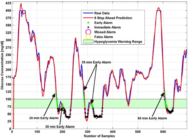
Early hypoglycemia alarm performance for 30 min predictions for subject 1

A hypoglycemic event is defined as continuous sequence of glucose concentration data below the selected threshold instead of individual data points. If there are more than two time steps between the groups of data that are below 70 mg/dl, they are considered two different hypoglycemic events. An alarm is also defined as a continuous event and considered true positive (TP) if it is issued up to 60 min before a real hypoglycemic event in patient data. The alarms raised during the event are not counted as early hypoglycemia alarm since our focus is in early detection. A false positive (FP) region is defined as the region where the alarm is triggered outside of the true positive region (long before or after a hypoglycemic event). An alarm is considered false negative (FN) if it is not raised inside the true positive region (60 min in advance of the beginning of the true hypoglycemic event). The early/advance detection time to the start of hypoglycemia episode is an important parameter in the evaluation of the alarm system and it indicates the period between the first warning signal for the future hypoglycemia episode and the potential occurrence time of the hypoglycemia episode. The time between the first alarm raised within the true positive region and the beginning of true hypoglycemic event is denoted by DT (detection times) in Tables 2-5.

Table 2.

Detailed Results for the Data from Subject 1 for Different Prediction Horizons

PH	NH	TP	FP	FN	DT	SSGPE	RMSE
1	5	2	0	3	10	0.349	0.713
2	5	4	0	1	12.5	0.974	1.987
3	5	5	0	0	17	1.877	3.829
4	5	5	0	0	24	3.023	6.167
5	5	5	0	0	30	4.412	9.004
6	5	5	0	0	35	6.015	12.278
7	5	5	1	0	40	7.831	15.988
8	5	5	2	0	42	9.835	20.083
9	5	5	2	0	45	12.024	24.559
10	5	5	2	0	46	14.376	29.367
11	5	5	3	0	48	16.883	34.494
12	5	5	3	0	49	19.525	39.898

PH: Prediction horizon, NH: Number of hypoglycemic events, TP: Number of true positive alarms, FP: Number of false positive alarms, FN: Number of false negative alarms, DT: Average detection time (minutes).

Table 5.

Detailed Results for All Subjects for Different Prediction Horizons in Real Time

PH	NH	S	FAR	DT	SSGPE	RMSE
1	201	0.480	0.333	32.69	0.998	1.860
2	201	0.535	0.319	32.64	2.267	4.237
3	201	0.635	0.309	29.35	3.844	7.183
4	201	0.700	0.317	28.53	5.617	10.499
5	201	0.760	0.324	28.02	7.695	14.399
6	201	0.815	0.343	29.06	9.911	18.551
7	201	0.855	0.359	30.87	12.324	23.075
8	201	0.890	0.384	32.18	14.849	27.818
9	201	0.910	0.403	34.45	17.537	32.867
10	201	0.920	0.444	35.15	20.301	38.061
11	201	0.939	0.450	37.13	23.173	43.462
12	201	0.959	0.475	37.98	26.079	48.935

PH: Prediction horizon, NH: Number of hypoglycemic events, S: Sensitivity, FAR: False alarm ratio, DT: Average detection time (minutes).

In Figure 1, all hypoglycemic events are predicted by the alarm system at least 30 minutes ahead of their occurrence. For this specific data set and prediction horizon there are no missed or false alarms.

The prediction error is expressed in terms of root mean squared error (RMSE):

$$\mathit{RMSE}=\sqrt{\frac{\sum {\left(y-\widehat{y}\right)}^2}{n}}$$ (19)

where ŷ is the predicted glucose concentration (mg/dl) by the model and n is the data length. The sum of squares of the glucose prediction error (SSGPE) is:

$$\mathit{SSGPE}=\sqrt{\frac{\sum {\left(y-\widehat{y}\right)}^2}{\sum y^2}}\times 100$$ (20)

Table 2 shows the number of early, missed and false alarms and the detection time for twelve different prediction horizons (PH) based on these evaluation criteria. For short prediction horizons, SSGPE and RMSE values are almost ideal, however some hypoglycemic events are missed and the average detection time is short for the predicted hypoglycemic events. As the prediction horizon is increased, SSGPE and RMSE values increase, indicating the increase in the difference between real and predicted values. Although the algorithm gives some false positive alarms for PH>6, there are no missed alarms for real hypoglycemic events. The 6-step-ahead PH is optimal for Subject 1 based on Table 2 with no missed and false alarms.

Only early hypoglycemia alarms are considered in the performance evaluation of our algorithm; alarms held during the event are not counted as true positive as CGMs are already equipped with immediate alarms for the current data point. Sensitivity, false positive ratio and time to detection are reported to assess the performance of the alarm system. Sensitivity is used as the measure of correctly identified positives and false positive ratio is defined to quantify false alarm rate per day. Sensitivity (S) of the alarm system is defined as the ratio of true early alarm to all hypoglycemic events:

$$S=\frac{\mathit{True\; Positive}}{\mathit{True\; Positive}+\mathit{False\; Negative}}$$ (21)

The false alarm ratio (FAR) is the fraction of the forecasts of the event associated with non-occurrences, as the name implies and is defined by:

$$\mathrm{FAR}=\frac{\mathit{False\; Positive}}{\mathit{True\; Positive}+\mathit{False\; Positive}}$$ (22)

Table 3 displays the results of all data-sets. 201 hypoglycemic events existed in the data analyzed. Most of these hypoglycemic events were predicted by the algorithm with 89.05% sensitivity and 28.6 min average detection time for PH=6. A warning 28.6 minutes in advance is more than enough time to take action for preventing hypoglycemia.

Table 3.

Detailed Results for Different Prediction Horizons for All Data

PH	NH	S	FAR	DT	SSGPE	RMSE
1	201	0.330	0	23.309	0.549	0.961
2	201	0.448	0.011	20.718	1.312	2.319
3	201	0.692	0.007	19.508	2.313	4.111
4	201	0.766	0.025	22.336	3.506	6.258
5	201	0.831	0.057	24.771	4.947	8.850
6	201	0.891	0.105	28.588	6.536	11.717
7	201	0.925	0.151	31.922	8.312	14.924
8	201	0.940	0.196	35.036	10.232	18.394
9	201	0.970	0.242	39.181	12.309	22.153
10	201	0.980	0.287	42.132	14.503	26.124
11	201	0.980	0.353	43.639	16.831	30.341
12	201	0.985	0.388	44.407	19.247	34.721

PH: Prediction horizon, NH: Number of hypoglycemic events, S: Sensitivity, FAR: False alarm ratio, DT: Average detection time (minutes).

Based on the proposed algorithm, a hypoglycemia early alarm system is proposed as illustrated in the flow chart in Figure 2. The alarm algorithm first checks the current data and if the glucose concentration is under the hypoglycemia threshold, an immediate hypoglycemia alarm is triggered. Then sleep or exercise conditions are checked. In case of sleep or exercise, the thresholds for signaling hypoglycemia are increased. This provides more time to compensate for potential hypoglycemia, since glucose values can decrease drastically and suddenly under these states. If a glucose value is higher than the defined threshold, the algorithm checks for predictions of future glucose values to determine the need to trigger a hypoglycemia early alarm. When the n-step-ahead predicted value crosses the hypoglycemia threshold a hypoglycemia early alarm is raised.

Figure 2.

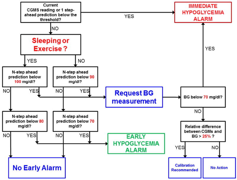
Early hypoglycemia alarm flow chart for real time implementation

Table 4 shows the results of the alarm system for data from Subject 1 in real time hypoglycemia detection. A Kalman filter is used for smoothing data. As in the offline case, the algorithm misses some hypoglycemic events for low prediction horizons. When the horizon is increased it can predict all hypoglycemic events but also trigger some false positive alarms. For the real-time case, again 6 steps (30 minutes) PH is optimal in terms of high detection time and low false positive alarm ratio.

Table 4.

Detailed Results for Subject 1 for Different Prediction Horizons in Real Time

PH	NH	TP	FP	FN	DT	SSGPE	RMSE
1	5	3	0	2	48.33	0.519	1.109
2	5	3	0	2	51.67	1.385	2.956
3	5	5	1	0	34.00	2.643	5.644
4	5	5	1	0	38.00	4.192	8.953
5	5	5	1	0	42.00	6.065	12.956
6	5	5	1	0	46.00	8.176	17.469
7	5	5	3	0	48.00	10.554	22.558
8	5	5	3	0	38.00	13.127	28.064
9	5	5	3	0	39.00	15.918	34.038
10	5	5	3	0	41.00	18.862	40.344
11	5	5	3	0	41.00	21.977	47.019
12	5	5	4	0	45.00	25.214	53.958

PH: Prediction horizon, NH: Number of hypoglycemic events, TP: Number of true positive alarms, FP: Number of false positive alarms, FN: Number of false negative alarms, DT: Average detection time (minutes).

Table 5 presents the result for all hypoglycemic events in real time. The sensitivity is lower but the detection time is higher compared to the offline case (Table 3). However, for PH=6 and higher, the algorithm is able to predict most of the hypoglycemic events with higher early detection time.

The performance of the ARMAX model based only on glucose measurements and ARMAX model based on glucose and physical activity information are compared in Table 6. The results are obtained using the real time approach. When the physical activity information is added to the ARMAX model the prediction error decreases significantly.

Table 6.

Predictions for Subject 1 Based on Single and Multivariable Models in Real Time

Variables used for predictions (PH: 6)	SSGPE	RMSE
Glucose (CGM)	19.266	41.169
Glucose (CGM) and EE, GSR (Armband)	8.603	18.383
Glucose (CGM), EE and GSR (Armband), and IOB	8.175	17.469

PH: Prediction horizon, EE: Energy expenditure, GSR: Galvanic skin response

Discussion of Results

Signal noise or unknown disturbances acting on a signal cause a lag in predicted values based on time series models, even if the model used is perfect. One way to overcome this issue is to use smoothed data for predictions. Usually a simple moving average (SMA) filter is used for extraction of smoothed data in real-time industrial applications. However, moving average causes a lag between raw and smoothed data equal to half of the window size of the filter. Exponential moving average (EMA) filter causes a smaller lag compared to SMA but it provides less smoothing. Also, moving average techniques are known to change the dynamics of the data at the peak points. Various techniques such as filtering raw data and implementing a second filter to the reversed filtered data from first filter or using future values of the data have been proposed to compensate the lag in EMA and SMA that are not possible to implement in real-time applications. IIR (Infinite Impulse Response) or FIR (Finite Impulse Response) filters are also known to create lags in real-time applications.

The Kalman filter provides optimal filtering, if the model of the process is known. However, the traditional Kalman filter assumes that both process and measurement disturbance to be white noise. Bequette²⁷ and Facchinetti et al.²⁸ proposed Kalman filters for real-time denoising of CGM data. In both studies, the Kalman filter can handle artificially created white noise on the signal. But when it is applied to real CGM data there is not a significant filtering of the signal. If the tuning parameters of the Kalman filter are defined to improve smoothing, then a lag appears between real and smoothed data. A non-causal Sativzky-Golay filter is known to be a least-squares-based filter that does not change the dynamics of the data even at the peak points. However, it has optimal performance only when the filtering window is selected half in the past and half in the future with respect to the time of the current data. Consequently, it has to be modified in real-time applications.³⁷ For example, the performance of the filter decreases and a lag is introduced if only the past half window of data is used. As long as only past data is used for filtering, any kind of real time filter causes a lag and this decreases filter performance and causes delay in alarm generation.

There is an inverse relationship between the amount of smoothing and lag created for any kind of real-time filter that use only past data. The tuning parameters Q and R of the Kalman filter defines the degree of smoothing. The larger the Q/R ratio, the lower is the smoothing applied to the data. On the other hand, the smaller the Q/R ratio, the larger is the lag created between filtered and raw data. Satisfactory smoothing is achieved when Q/R is 10^-5 or smaller. But for these tuning parameters, the lag is too large for use in alarm systems. For larger Q/R ratio, the lag is reduced but there is not enough smoothing of the data. This inverse relation explains why SSGPE and RMSE values are larger in the real-time case and the lag causes some missed alarms which decrease the sensitivity of the early warning system.

There is no ideal filtering algorithm that creates no lag while providing good data smoothing in real-time. But it is highly expected from next generation of CGM devices to reduce measurement noise. This would improve the performance of prediction algorithms and early hypoglycemia warning systems.

A better prediction of BGC can be obtained by using additional physiological signals.¹⁰ Moreover, use of physiological signals enables the alarm system to be aware of the time periods with high probability of hypoglycemia such as sleep or post-exercise periods. An alarm system based only on glucose values would issue an alarm only when the BGC predictions are low. In the proposed multivariable alarm system and its extensions for closed-loop systems^{14, 16}, an alarm or low insulin amounts are suggested even when the predictions have not approached the alarm thresholds, but the trends are detected. The system predicts the post-exercise glucose decrease that has not been seen in the trend of glucose readings yet.

Conclusions

Early alarms to warn the potential of hypoglycemia are important for the acceptance of artificial pancreas systems and assistance to parents of young children with T1D. They can provide enough time to take action to avoid hypoglycemia. A subject-specific recursive linear time series modeling technique is used to develop models for predicting future BGC. Savitzky-Golay filters and Kalman filters are used to reduce noise in patient data. The modeling algorithm enables dynamic adaptation of models to inter-/intra-subject variations and glycemic disturbances, and provides satisfactory BGC prediction with relatively small error.

These models are used in hypoglycemia early alarm systems. The models developed and the hypoglycemia warning system is tested retrospectively using T1D subject data. Good filtering algorithms that create small lags while providing data smoothing in real-time are needed to improve the BGC predictions and the performance of hypoglycemia alarm systems. While such filters are not currently available, hardware improvements of next generation of CGM devices are expected to reduce measurement noise. The alarm system developed has a good performance in prediction of hypoglycemia and ultimately in prevention of its occurrence.

Table 1.

Time Series Model Parameters and Orders, and Values Selected

Parameters	Values
nA, nB1, nB2, nB3, nc	3, 11, 3, 3, 1
d1, d2, d3	1, 2, 2
θ̂(0)	024×1
P(0)	100×I24×24
λ	0.98
IOB	2 h IOB curve
θmax	[1 1 1 01×12 01×4 01×4 1]T
θmin	[−1 −1 −1 IOBcrv −11×4 −11×4 −1]T

References

- 1.Centers for Disease; Control; Prevention. National Diabetes Fact Sheet: National Estimates and General Information on Diabetes and Prediabetes in the United States, 2011. US Department of Health and Human Services; 2011. [Google Scholar]
- 2.Buckingham B, Chase HP, Dassau E, Cobry E, Clinton P, Gage V, Caswell K, Wilkinson J, Cameron F, Lee H, Bequette BW, Doyle FJ., III Prevention of Nocturnal Hypoglycemia Using Predictive Alarm Algorithms and Insulin Pump Suspension. Diabetes Care. 2010;33(5):1013–7. doi: 10.2337/dc09-2303. [DOI] [PMC free article] [PubMed] [Google Scholar]
- 3.Buckingham B, Cobry E, Clinton P, Gage V, Caswell K, Kunselman E, Cameron F, Chase HP. Preventing Hypoglycemia Using Predictive Alarm Algorithms and Insulin Pump Suspension. Diabetes Technol Ther. 2009;11(2):93–97. doi: 10.1089/dia.2008.0032. [DOI] [PMC free article] [PubMed] [Google Scholar]
- 4.Agrawal P, Welsh JB, Kannard B, Askari S, Yang Q, Kaufman FR. Usage and Effectiveness of the Low Glucose Suspend Feature of the Medtronic Paradigm Veo Insulin Pump. J Diabetes Sci Technol. 2011;5(5):1137–41. doi: 10.1177/193229681100500514. [DOI] [PMC free article] [PubMed] [Google Scholar]
- 5.Cameron F, Wilson DM, Buckingham BA, Arzumanyan H, Clinton P, Chase HP, Lum J, Maahs DM, Calhoun PM, Bequette BW. Inpatient Studies of a Kalman-Filter-Based Predictive Pump Shutoff Algorithm. J Diabetes Sci Technol. 2012;6(5):1142–7. doi: 10.1177/193229681200600519. [DOI] [PMC free article] [PubMed] [Google Scholar]
- 6.Palerm CC, Bequette BW. Hypoglycemia Detection and Prediction Using Continuous Glucose Monitoring-a Study on Hypoglycemic Clamp Data. J Diabetes Sci Technol. 2007;1(5):624–629. doi: 10.1177/193229680700100505. [DOI] [PMC free article] [PubMed] [Google Scholar]
- 7.Palerm CC, Willis JP, Desemone J, Bequette BW. Hypoglycemia Prediction and Detection Using Optimal Estimation. Diabetes Technol Ther. 2005;7(1):3–14. doi: 10.1089/dia.2005.7.3. [DOI] [PubMed] [Google Scholar]
- 8.Sparacino G, Zanderigo F, Corazza S, Maran A, Facchinetti A, Cobelli C. Glucose Concentration Can Be Predicted Ahead in Time from Continuous Glucose Monitoring Sensor Time-Series. IEEE Trans Biomed Eng. 2007;54(5):931–937. doi: 10.1109/TBME.2006.889774. [DOI] [PubMed] [Google Scholar]
- 9.Eren-Oruklu M, Cinar A, Quinn L, Smith D. Estimation of Future Glucose Concentrations with Subject-Specific Recursive Linear Models. Diabetes Technol Ther. 2009;11(4):243–253. doi: 10.1089/dia.2008.0065. [DOI] [PMC free article] [PubMed] [Google Scholar]
- 10.Eren-Oruklu M, Cinar A, Rollins DK, Quinn L. Adaptive System Identification for Estimating Future Glucose Concentrations and Hypoglycemia Alarms. Automatica. 2012;48(8):1892–1897. doi: 10.1016/j.automatica.2012.05.076. [DOI] [PMC free article] [PubMed] [Google Scholar]
- 11.Dassau E, Cameron F, Lee H, Bequette BW, Zisser H, Jovanovic L, Chase HP, Wilson DM, Buckingham BA, Doyle FJ., III Real-Time Hypoglycemia Prediction Suite Using Continuous Glucose Monitoring: A Safety Net for the Artificial Pancreas. Diabetes Care. 2010;33(6):1249–54. doi: 10.2337/dc09-1487. [DOI] [PMC free article] [PubMed] [Google Scholar]
- 12.Cameron F, Niemeyer G, Gundy-Burlet K, Buckingham B. Statistical Hypoglycemia Prediction. J Diabetes Sci Technol. 2008;2(4):612–21. doi: 10.1177/193229680800200412. [DOI] [PMC free article] [PubMed] [Google Scholar]
- 13.Bayrak ES, Turksoy K, Cinar A, Quinn L, Littlejohn E, Rollins D. Hypoglycemia Early Alarm Systems Based on Recursive Autoregressive Partial Least Squares Models. Journal of Diabetes Science and Technology. 2012;7(1):206–214. doi: 10.1177/193229681300700126. [DOI] [PMC free article] [PubMed] [Google Scholar]
- 14.Turksoy K, Bayrak ES, Quinn L, Littlejohn E, Cinar A. Multivariable Adaptive Closed-Loop Control of an Artificial Pancreas without Meal and Activity Announcement. Diabetes Technology & Therapeutics. 2013;15(5) doi: 10.1089/dia.2012.0283. Ahead of print. [DOI] [PMC free article] [PubMed] [Google Scholar]
- 15.Box GEP, MacGregor JF. Parameter Estimation with Closed-Loop Operating Data. Technometrics. 1976;18(4):371–380. [Google Scholar]
- 16.Turksoy K, Bayrak ES, Quinn L, Littlejohn E, Cinar A. Adaptive Multivariable Closed-Loop Control of Blood Glucose Concentration in Patients with Type 1 Diabetes. Proc 2013 American Control Conf; Washington, DC.. 2013. Accepted. [Google Scholar]
- 17.Sohlberg B. Applied Modelling and Identification. Bindomatic. 2008 [Google Scholar]
- 18.Box GEP, MacGregor JF. The Analysis of Closed-Loop Dynamic-Stochastic Systems. Technometrics. 1974;16(3):391–398. [Google Scholar]
- 19.Lütkepohl H. New Introduction to Multiple Time Series Analysis. Springer; 2006. [Google Scholar]
- 20.Badwe AS, Singh A, Patwardhan SC, Gudi RD. A Constrained Recursive Pseudo-Linear Regression Scheme for on-Line Parameter Estimation in Adaptive Control. Journal of Process Control. 2010;20(5):559–572. [Google Scholar]
- 21.Aström KJ, Wittenmark B. Computer-Controlled Systems: Theory and Design. Courier Dover Publications; 2011. [Google Scholar]
- 22.Favier G, Dubois D. A Review of K-Step-Ahead Predictors. Automatica. 1990;26(1):75–84. [Google Scholar]
- 23.De Keyser RMC, Van Cauwenberghe AR. A Self-Tuning Multistep Predictor Application. Automatica. 1981;17(1):167–174. [Google Scholar]
- 24.Lacy SL, Bernstein DS. Subspace Identification with Guaranteed Stability Using Constrained Optimization. IEEE T Automat Contr. 2003;48(7):1259–1263. [Google Scholar]
- 25.Walsh J, Roberts R. Pumping Insulin. Torrey Pines Press; 2006. [Google Scholar]
- 26.Savitzky A, Golay MJE. Smoothing and Differentiation of Data by Simplified Least Squares Procedures. Analytical chemistry. 1964;36(8):1627–1639. [Google Scholar]
- 27.Bequette BW. Continuous Glucose Monitoring: Real-Time Algorithms for Calibration, Filtering, and Alarms. J Diabetes Sci Technol. 2010;4(2):404–18. doi: 10.1177/193229681000400222. [DOI] [PMC free article] [PubMed] [Google Scholar]
- 28.Facchinetti A, Sparacino G, Cobelli C. An Online Self-Tunable Method to Denoise Cgm Sensor Data. IEEE T Bio-Med Eng. 2010;57(3):634–641. doi: 10.1109/TBME.2009.2033264. [DOI] [PubMed] [Google Scholar]
- 29.Banarer S, Cryer PE. Sleep-Related Hypoglycemia-Associated Autonomic Failure in Type 1 Diabetes Reduced Awakening from Sleep During Hypoglycemia. Diabetes. 2003;52(5):1195–1203. doi: 10.2337/diabetes.52.5.1195. [DOI] [PubMed] [Google Scholar]
- 30.Maltoni G, Zucchini S, Scipione M, Rollo A, Balsamo C, Bertolini C, Baronio F, Rondelli R, Pession A. Severe Hypoglycemic Episodes: A Persistent Threat for Children with Type 1 Diabetes Mellitus and Their Families. Journal of endocrinological investigation. 2013 doi: 10.3275/8896. Ahead of print. [DOI] [PubMed] [Google Scholar]
- 31.Bequette BW. Challenges and Recent Progress in the Development of a Closed-Loop Artificial Pancreas. Annual Reviews in Control. 2012;36(2):255–266. doi: 10.1016/j.arcontrol.2012.09.007. [DOI] [PMC free article] [PubMed] [Google Scholar]
- 32.MacDonald MJ. Postexercise Late-Onset Hypoglycemia in Insulin-Dependent Diabetic Patients. Diabetes Care. 1987;10(5):584–588. doi: 10.2337/diacare.10.5.584. [DOI] [PubMed] [Google Scholar]
- 33.Yardley JE, Iscoe KE, Sigal RJ, Kenny GP, Perkins BA, Riddell MC. Insulin Pump Therapy Is Associated with Less Post-Exercise Hyperglycemia Than Multiple Daily Injections: An Observational Study of Physically Active Type 1 Diabetes Patients. Diabetes Technol Ther. 2013;15(1):84–8. doi: 10.1089/dia.2012.0168. [DOI] [PubMed] [Google Scholar]
- 34.Riddell MC, Milliken J. Preventing Exercise-Induced Hypoglycemia in Type 1 Diabetes Using Real-Time Continuous Glucose Monitoring and a New Carbohydrate Intake Algorithm: An Observational Field Study. Diabetes Technol Ther. 2011;13(8):819–25. doi: 10.1089/dia.2011.0052. [DOI] [PubMed] [Google Scholar]
- 35.Kelly D, Hamilton JK, Riddell MC. Blood Glucose Levels and Performance in a Sports Camp for Adolescents with Type 1 Diabetes Mellitus: A Field Study. Int J Pediatr. 2010 doi: 10.1155/2010/216167. Article ID 216167. [DOI] [PMC free article] [PubMed] [Google Scholar]
- 36.Riddell MC, Iscoe KE. Physical Activity, Sport, and Pediatric Diabetes. Pediatr Diabetes. 2006;7(1):60–70. doi: 10.1111/j.1399-543X.2006.00146.x. [DOI] [PubMed] [Google Scholar]
- 37.Rajagopalan R. Generalized Causal Moving Average (GCMA) Smoothing Filter for Real-Time Applications. Proc SPIE 5205, Advanced Signal Processing Algorithms, Architectures, and Implementations XIII. 2003;426 doi: 10.1117/12.509703. [DOI] [Google Scholar]