Adjusting for unknown bias in non-inferiority clinical trials

Abstract

Evaluation of non-inferiority is based on ruling out a threshold for what would constitute unacceptable loss of efficacy of an experimental treatment relative to an active comparator “Standard”. This threshold, the “non-inferiority margin”, is often based on preservation of a percentage of Standard’s effect. To obtain an estimate of this effect to be used in the development of the “non-inferiority margin”, data are needed from earlier trials comparing Standard to placebo if the non-inferiority trial does not have a placebo arm. This approach often provides a biased over-estimate of Standard’s true effect in the setting of the current non-inferiority study. We describe two commonly used non-inferiority margin methods that adjust for this bias, the two-confidence interval (95-95) and the Synthesis margins. However, the added ‘variance inflation’ adjustment made by 95-95 margin diminishes with increasing information from historical trial(s), and the Synthesis margin is based on a strong assumption that the relative bias is known. We introduce an alternative “Bias-adjusted” margin addressing vulnerabilities of each by attenuating the estimate and by accounting for uncertainty in the true level of bias. Examples and asymptotic estimates of non-inferiority hypothesis rejection rates in the proportional hazards setting are used to compare methods.

1 Background

Non-inferiority clinical trials are designed to compare an experimental therapy (Experimental) to a standard treatment (Standard), allowing for a maximal acceptable loss of efficacy of Experimental relative to Standard, called the non-inferiority margin (Δ). In the regulatory non-inferiority trial setting, tests for Experimental efficacy are most often conducted using margin based methods which rely on a historical estimate of the effect of Standard relative to placebo or best standard of care (Placebo). [1, 2, 3]

In March 2010, the Food and Drug Administration issued a Draft Guidance for Industry on non-inferiority clinical trials. In this guidance, the Agency discusses two sources of uncertainty that need to be addressed regarding the effect of Standard relative to Placebo. First, estimates based on results from one or more historical trials will have statistical variability. Second, the effect of Standard estimated from past studies may be ‘different from (larger than) the effect of the active control in the current non-inferiority study.’[4]

The latter concern results in part from violation of the ‘constancy assumption’, that the true effect of Standard is the same in the historical and non-inferiority trial settings. Bias in the estimate of Standard relative to Placebo can arise, not only due failure of the constancy assumption but also from issues such as exclusion of unpublished ‘negative’ results from clinical trials, selection of the control with the greatest estimated effect from among a class of available treatments, and ‘cherry picking’ for use in meta-analysis the favorable results from among trials or subgroups within trials. These biases tend to over-estimate the effect of Standard, and failure to account for them may lead to increased risk of use of insufficiently effective or ineffective therapies.[1, 5]

In this article, we will consider the non-inferiority setting where it has been deemed unethical for a Placebo to be included in the non-inferiority trial. After introducing notation, we will describe two commonly used margin formulation methods that employ estimates of Standard relative to Placebo from earlier trials. We will compare approaches to adjust these margins for bias, and then propose a margin method which addresses vulnerabilities of the existing adjusted methods. Finally, we will evaluate margins with respect to asymptotic approximations of across-trial non-inferiority hypothesis test rejection rates under settings motivated by real-world examples.

2 Notation

Let μ_X and μ_Y denote continuous parameters for an outcome measure for subjects in a clinical trial on treatments X and Y respectively. Then, suppose that β_XY ≡ μ_X − μ_Y is the parameter of interest comparing treatments X and Y. By definition, β_XY = −β_YX. One example of μ is the natural log of the hazard, and β is the corresponding natural log hazard ratio. Other examples for β include the natural log of the odds ratio, the difference in proportions, or the difference in means for some clinical measure of interest.

Let β_ES denote the true effect of Experimental relative to Standard, β_SP denote the true effect of Standard relative to Placebo, and β_EP denote the true effect of Experimental relative to Placebo, all in the setting of the non-inferiority trial. Assume that β_ES , β_EP, and β_SP are negative when Experimental is more efficacious than Standard, when Experimental is more efficacious than Placebo, and when Standard is more efficacious than Placebo. Also note that β_PS, which is equal to −β_SP , would be the margin for ruling out loss of the entire effect of Standard relative to Placebo in the absence of uncertainty.

Assume β̂_ES is the estimate of β_ES obtained using data from the non-inferiority trial, and β̂_PS,H is the estimate of β_PS obtained using data from one (or more) well designed and conducted trial(s) evaluating the effect of Standard relative to Placebo and that these estimates are independently distributed. When β̂_PS,H is biased for β_PS, this bias can be expressed in terms of a multiple of the expectation of β̂_PS,H, E[β̂_PS,H]. So, for some λ ≠ 0

$$(1-\lambda )E[{\widehat{\beta }}_{PS,H}]={\beta }_{PS}$$ (1)

Suppose we want to conduct the test defined by the following null, H₀′, and alternative, H_a′, hypotheses:

$$\begin{array}{c}{H_0}^{\prime }:{\beta }_{ES}\ge \mathrm{\Delta }\\ {H_a}^{\prime }:{\beta }_{ES}\le {\mathrm{\Delta }}_a\text{for}\text{some}\text{specified}{\mathrm{\Delta }}_a<\mathrm{\Delta }\end{array}$$

where Δ is the non-inferiority margin. Often Δ_a is taken to be 0.

When β̂_ES is approximately normally distributed with variance estimate v̂ar(β̂_ES), the approximate level alpha test for H₀′ versus H_a′ rejects when

$${\widehat{\beta }}_{ES}+z_{1-\alpha }\sqrt{\widehat{v}ar({\widehat{\beta }}_{ES})}<\mathrm{\Delta }$$ (2)

We will frame margins in the context of the rejection region in expression (2) for consistency with the Food and Drug Administration guidance document and to allow for direct comparison of methods. We will also carefully address the following Considerations in development of the non-inferiority margin [6]:

1. The non-inferiority margin should be formulated using adjustments to account for bias or lack of reliability in the estimate of the effect of Standard in the non-inferiority trial setting.

2. The non-inferiority margin should be formulated to achieve preservation of an appropriate percentage of the effect of Standard.

When addressing Consideration B, we will use p to denote the proportion of β_PS to be preserved.

3 Current margin methods for assessment of non-inferiority and adjustment for bias

3.1 95-95 confidence interval margin

When choosing Δ as described in the prior section, one might address Consideration A by taking the lower limit of the confidence interval (CI) for the estimate of Placebo relative to Standard from available data as an intermediate margin “M₁ ”, and apply Consideration B by taking Δ ≡ (1 − p)M₁ , where p is a preservation of effect fraction. This process results in a test rejecting when

$${\widehat{\beta }}_{ES}+z_{1-\alpha }{(\widehat{v}ar{\widehat{\beta }}_{ES})}^{1/2}<(1-p)[{\widehat{\beta }}_{PS,H}-z_{1-\alpha }{(\widehat{v}ar{\widehat{\beta }}_{PS,H})}^{1/2}]$$ (3)

When the one-sided α is equal to 0.025 (equivalent to two-sided α of 0.05), the right hand side of equation (3) is the “95-95” CI margin. This margin is also called the Fixed margin since the values of β̂_PS,H and v̂arβ̂_PS,H are known prior to design and conduct of the non-inferiority trial. Though Considerations A and B are treated as separate steps for development of Δ in (3), they may instead be considered simultaneously in the development of the final margin.

3.2 Synthesis Margin

An alternative approach can be formulated for a setting under presumed certainty of an unbiased estimate of the effect of Standard in the non-inferiority trial setting.

Suppose we wish to ensure preservation of a fraction p of the effect of Standard, as in Consideration B, then the relevant hypotheses H₀ and H_a are:

$$\begin{array}{c}{H}_0:{\beta }_{EP}\ge p{\beta }_{SP}\\ H_a:{\beta }_{EP}\le p_a{\beta }_{SP}\text{for}\text{some}\text{specified}{p}_a>p\end{array}$$

which, with β_EP = β_ES + β_SP = β_ES − β_PS , is equivalent to:

$$\begin{array}{c}{H_0}^{\ast }:{\beta }_{ES}-(1-p){\beta }_{PS}\ge 0\\ {H_a}^{\ast }:{\beta }_{ES}-(1-p_a){\beta }_{PS}\le 0\text{for}\text{specified}{p}_a>p\end{array}$$

Often p_a is taken to be 1; then, the alternatives H_a and H_a* are equivalent to H_a′ with Δ_a equal to 0. With unbiased, normally distributed estimates β̂_ES and β̂_PS,H and with corresponding variances var(β̂_ES) and var(β̂_PS,H) , the natural level-α test for H₀ versus H_a rejects when

$$\frac{{\widehat{\beta }}_{ES}-(1-p){\widehat{\beta }}_{PS,H}}{\sqrt{\mathit{var}({\widehat{\beta }}_{ES})+{(1-p)}^2\mathit{var}({\widehat{\beta }}_{PS,H})}}<-z_{1-\alpha }$$ (4)

Recognizing asymptotic normality for unbiased estimates β̂_ES and β̂_PS,H and substituting consistent estimators v̂ar(β̂_ES) and v̂ar(β̂_PS,H) for var(β̂_ES) and var(β̂_PS,H) leads to a test that is asymptotically size α and corresponds to (2) with Δ equal to

$$(1-p){\widehat{\beta }}_{PS,H}-z_{1-\alpha }[\sqrt{\widehat{v}ar({\widehat{\beta }}_{ES})+{(1-p)}^2\widehat{v}ar({\widehat{\beta }}_{PS,H})}-\sqrt{\widehat{v}ar({\widehat{\beta }}_{ES})}]$$ (5)

Expression (5) is the commonly used form of the Synthesis margin with preservation of proportion p of the effect of Standard relative to Placebo. [2] This formulation of the Synthesis method, named due to the “synthesis” of results from the non-inferiority and historical trials, allows direct comparison to the 95-95 margin and to other margins.

Margin development and assessment of non-inferiority by the 95-95 and Synthesis methods are contrasted in Figure 1, using the example of evaluation of bivalirudin efficacy on the endpoint of death, MI or urgent revascularization by day 30 in the setting of percutaneous coronary interventions. Data are from the REPLACE 2 non-inferiority trial and from the historical EPISTENT and ESPRIT trials that are used to estimate the effect of the Glycoprotein IIb/IIIa inhibitor that is “Standard”.[1] In panel 1a, the lined region (to the right) represents the 95% CI for the odds ratio on “Placebo” compared to “Standard” in the context of background heparin treatment, using data from EPISTENT and ESPRIT, and the lower limit of this interval, exp(M₁), is the intermediate 95-95 (p = 0) margin on the odds ratio scale. In panel 1b, Experimental is compared to Placebo indirectly by the Synthesis method, with no preservation of effect. Panels 2a and 2b depict 95-95 and Synthesis margin development under preservation of 50% of the effect of Standard relative to Placebo. The 95-95 margin of 1.19 is obtained by taking the lower limit of the CI for 0.5β_PS , equal to exp(0.5M₁), and the Synthesis margin of 1.30 is obtained by the formula shown below the panels. Both 1.19 and 1.30 are examples of (exponentiated) margins for testing H₀. Though Experimental fails to preserve 50% of the effect of Standard by either method, the Synthesis comparison is less strict, with the lower limit of the CI shown in panel 2b only slightly below 1, and correspondingly the upper limit of the shaded region in panel 2a only slightly above 1.30.

Figure 1.

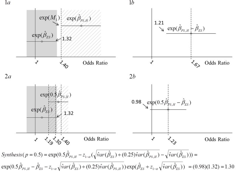
Depiction of 95-95 and Synthesis margins’ development in the example of evaluation of bivalirudin efficacy from REPLACE 2 non-inferiority trial and from the EPISTENT and ESPRIT trials. In panels 1a and 2a, the shaded region (the left-side region of each panel) represents the 95% confidence interval for the Odds Ratio for Events on Experimental relative to Standard, with Experimental better than Standard if the Odds Ratio is less than 1. In panel 1a, the lined region represents the 95% confidence interval for the odds ratio on Placebo compared to Standard, with background heparin therapy on both arms, from EPISTENT and ESPRIT, and the lower limit of this interval is exp(M₁). In panel 1b, Experimental is compared to Placebo indirectly by the Synthesis method. Panels 2a and 2b depict 95-95 and Synthesis margin development under preservation of 50% of the effect of Standard relative to Placebo.

3.3 The Synthesis(λ, p) margin and adjustment for bias

Rothmann et al. suggested that with known θ ≡ 1 − λ, the margin may be directly adjusted by correcting the estimate and using the corresponding standard error.[2] The resulting margin is:

$$(1-p)\theta {\widehat{\beta }}_{PS,H}-z_{1-\alpha }[\sqrt{\widehat{v}ar{\widehat{\beta }}_{ES}+{(1-p)}^2{\theta }^2\widehat{v}ar{\widehat{\beta }}_{PS,H}}-\sqrt{\widehat{v}ar{\widehat{\beta }}_{ES}}]$$ (6)

which, since by definition θ =1 − λ, is equivalent to

$$(1-p)(1-\lambda ){\widehat{\beta }}_{PS,H}-z_{1-\alpha }[\sqrt{\widehat{v}ar{\widehat{\beta }}_{ES}+{(1-p)}^2{(1-\lambda )}^2\widehat{v}ar{\widehat{\beta }}_{PS,H}}-\sqrt{\widehat{v}ar{\widehat{\beta }}_{ES}}]$$ (7)

The margin given by (7) will be referred to as Synthesis(λ, p). When we do not specify λ, assume that the default is 0, as given by (5), and that no bias adjustment is made for likely bias in estimation of β_PS. If we do not specify p, then the default value is 0.5, corresponding to preservation of half of the effect of Standard relative to Placebo. When the Synthesis margin is advocated in the literature, the authors usually appear to be using the unadjusted(λ = 0) margin. However, in some discussions only a ‘discounting’ factor is applied with no preservation of effect. [7, 8] Snapinn and Jiang (2008) argued in favor of the latter setting and suggested only a discounting factor incorporating NI trial estimate bias (“assay sensitivity”) as well as historical estimate bias. [8] Fleming et al. (2011) emphasized the need for preservation of effect, in addition to addressing the risk for bias, especially when the active comparator has demonstrated efficacy with respect to irreversable morbidity or mortality. [6] Wiens (2002) suggested use of a larger p to account for both Considerations A and B at once. [9] Though Synthesis(λ, p) is equivalent to use of a single multiplicative factor, (1 − p)(1 − λ) , distinguishing between bias and preservation of effect provides clarity.

3.4 95-95 and Synthesis(λ, p) Adjustment Limitations

Like the Synthesis(λ =0, p) method, the 95-95 CI method for formulation of the margin in the context of the hypothesis test defined by H₀ and H_a makes adjustments for the variability of the historical estimates and addresses the preservation of proportion p of the effect of Standard.[4] However, relative to Synthesis(λ = 0, p), the 95-95 CI method also “provides robustness” which may be considered adjustment for uncertainty in the unbiasedness of historical estimates.[4, 9] As shown by Fleming (2008), the difference between (3) and (5) suggests that the added adjustment that is made by the 95-95 method relative to Synthesis(λ = 0, p), is the non-negative term

$$z_{1-\alpha }\{{[A+B+2\sqrt{A}\sqrt{B}]}^{1/2}-{[A+B]}^{1/2}\}$$ (8)

where A ≡ v̂arβ̂_ES and where B ≡ (1 − p)² v̂arβ̂_PS,H.[1] This adjustment depends on the variances of estimates from the non-inferiority trial and the historical trials rather than being a direct function of bias in the effect of Standard relative to Placebo.

In contrast, the Synthesis(λ, p) margin directly adjusts the estimated effect of Standard and has across-trial size α for testing H₀ versus H_a when λ is known. However, λ is generally unknown, and for a given set of estimates and their variances, Synthesis(0 < λ < 1, p) may actually be greater than Synthesis(λ = 0, p).

Synthesis(0 < λ < 1, p) is greater than Synthesis(λ = 0, p) when the following inequality holds:

$$(1-p)\lambda {\widehat{\beta }}_{PS,H}-z_{1-\alpha }[\sqrt{\widehat{v}ar{\widehat{\beta }}_{ES}+{(1-p)}^2\widehat{v}ar{\widehat{\beta }}_{PS,H}}-\sqrt{\widehat{v}ar{\widehat{\beta }}_{ES}+{(1-p)}^2{(1-\lambda )}^2\widehat{v}ar{\widehat{\beta }}_{PS,H}}]<0$$ (9)

This phenomenon was observed in an example under which the historical estimate of Standard effect just failed to reach significance and a test for superiority would be recommended.[5] The fact that the Synthesis(0 < λ < 1, p) margin adjustment relative to Synthesis(λ = 0, p) may be “anti-conservative” under (9) is problematic, since both λ and v̂ar(β̂_ES) may be specified by the sponsor during protocol development, after β̂_PS,H and v̂ar(β̂_PS,H) are known.

We can directly attenuate the estimated effect of Standard in order to account for unknown bias while reducing the sensitivity of the adjustment to variances of the trials by using the method proposed in the following section.

4 Proposed method and comparison to existing margins

4.1 Proposed ‘Bias-adjusted’ Margin

Synthesis(λ, p) makes an adjustment that is appropriate when λ is known, yet λ is unknown. Suppose we assume λ is independent of β̂_PS,H and normally distributed with mean λ₀ and variance τ². Then we may obtain the mean and variance of (1 − λ)β̂_PS,H using properties of products of random variables. Substituting the mean and variance of (1 − λ)β̂_PS,H under this model with random λ leads to the following Synthesis margin:

$$(1-p)(1-{\lambda }_0){\widehat{\beta }}_{PS,H}-z_{1-\alpha }\{\sqrt{\widehat{v}ar{\widehat{\beta }}_{ES}+{(1-p)}^{2}V}-\sqrt{\widehat{v}ar{\widehat{\beta }}_{ES}}\}$$ (10)

where $V\equiv {(1-{\lambda }_0)}^2\widehat{v}ar{\widehat{\beta }}_{PS,H}+{\widehat{\beta }}_{PS,H}^2{\tau }^2+\widehat{v}ar{\widehat{\beta }}_{PS,H}{\tau }^2$.

Unfortunately, this form of the margin introduces another parameter to be specified, τ², which is not directly estimable from the non-inferiority trial. When ${\tau }^2=\frac{(1-{(1-{\lambda }_0)}^2)\widehat{v}ar{\widehat{\beta }}_{PS,H}}{{{\widehat{\beta }}_{PS,H}}^2+\widehat{v}ar{\widehat{\beta }}_{PS,H}}$, a test using (10) is equivalent to holding the confidence width for β̂_PS,H fixed. This relationship reflects increasing uncertainty about the true bias proportion λ with increasing expected bias proportion λ₀ and is equivalent to multiplying the first term of the unadjusted Synthesis margin by 1 − λ₀ as shown below

$$(1-p)(1-{\lambda }_0){\widehat{\beta }}_{PS,H}-z_{1-\alpha }[\sqrt{\widehat{v}ar({\widehat{\beta }}_{ES})+{(1-p)}^2\widehat{v}ar({\widehat{\beta }}_{PS,H})}-\sqrt{\widehat{v}ar({\widehat{\beta }}_{ES})}]$$ (11)

Expression (11) is a margin which adjusts for expected bias and variability in estimation of the effect of Standard relative to Placebo in the setting of the non-inferiority trial. It also preserves a portion of the effect of Standard, thereby addressing both Considerations A and B. We will call this the “Bias-adjusted(λ, p)” margin.

Figure 2 illustrates how different assumptions about bias proportions change the confidence interval for the effect of Standard to Placebo in the setting of the non-inferiority trial for the bivalirudin example presented in Figure 1. In each of the three panels A, B, and C, the lined region (on the right side of each panel) represents the 95% CI for β_PS under different assumptions about λ, the amount by which β̂_PS,H is biased for β_PS. The value of τ² in panel C maintains the width of the confidence interval from panel A, reflecting uncertainty about the true value of λ as described above.

Figure 2.

Diagrams showing how different assumptions about bias proportions change the confidence interval for the effect of Standard to Placebo in the setting of the non-inferiority trial. In each of the three panels A, B, and C, the lined region (on the right side of each panel) represents the 95% confidence interval for β_PS under different assumptions about λ, the amount by which β̂_PS,H is biased for β_PS. The value of τ² in panel C maintains the width of the confidence interval from panel A, reflecting uncertainty about the true value of λ.

As discussed by Fleming, several inconsistencies between the bivalirudin NI trial and historical trials existed, including differences in patient characteristics, use of supportive care, dose, schedule, level of adherence, and composite endpoint definitions.[1] These differences suggest that the estimate of effect of Standard from prior trials is likely positively biased in the setting of the NI trial; however, this bias cannot be directly assessed. Suppose the comparison to the 95-95 margin for examples obtained from a systematic review of trials discussed at advisory committee meetings, shown in the Appendix, is used to provide a context for the choice of λ. Using this reference, we take λ equal to 0.3, and apply the “Bias-adjusted(0.3, 0.5)” margin given by (11). This leads to a margin equal to (0.5)(0.7)(ln(1.82)) − 1.96 [√(0.01 + 0.25*0.017) − √(0.01)], which on the Odds Ratio scale is approximately equal to the 95-95 margin of 1.19.

4.2 Analytical comparison to existing methods

The difference between Bias-adjusted(λ, p) and Synthesis(λ = 0, p) is:

$$\lambda (1-p){\widehat{\beta }}_{PS,H}$$ (12)

Note that this difference is non-negative as long as β̂_PS,H is non-negative, p is in the range [0,1], and λ ≥ 0. This term represents the added adjustment of the new margin for suspected bias in β̂_PS,H.

If we compare Bias-adjusted(λ_B, p) and Synthesis(λ_S , p), we have the difference:

$$(1-p)({\lambda }_B-{\lambda }_S){\widehat{\beta }}_{PS,H}-z_{1-\alpha }[{(\widehat{v}ar{\widehat{\beta }}_{ES}+{(1-p)}^2\widehat{v}ar{\widehat{\beta }}_{PS,H})}^{1/2}-{(\widehat{v}ar{\widehat{\beta }}_{ES}+{(1-p)}^2{(1-{\lambda }_S)}^2\widehat{v}ar{\widehat{\beta }}_{PS,H})}^{1/2}]$$ (13)

If λ_B = λ_S = λ, then the difference is

$$-z_{1-\alpha }[{(\widehat{v}ar{\widehat{\beta }}_{ES}+{(1-p)}^2\widehat{v}ar{\widehat{\beta }}_{PS,H})}^{1/2}-{(\widehat{v}ar{\widehat{\beta }}_{ES}+{(1-p)}^2{(1-\lambda )}^2\widehat{v}ar{\widehat{\beta }}_{PS,H})}^{1/2}]$$ (14)

In this case, Bias-adjusted(λ, p) converges to Synthesis(λ, p) as v̂ar(β̂_PS,H) converges to zero. We now compare (14) to the adjustment made by the 95-95 method relative to Synthesis(0, p) to obtain:

$$-\lambda (1-p){\widehat{\beta }}_{PS,H}+z_{1-\alpha }\{{[A+B+2\sqrt{A}\sqrt{B}]}^{1/2}-{[A+B]}^{1/2}\}$$ (15)

where A ≡ v̂arβ̂_ES and where B ≡ (1 − p)² v̂arβ̂_PS,H as in expression (8).

This term may be negative when:

$$\lambda (1-p){\widehat{\beta }}_{PS,H}>z_{1-\alpha }\{{[A+B+2\sqrt{A}\sqrt{B}]}^{1/2}-{[A+B]}^{1/2}\}$$ (16)

Thus, the new margin may be more conservative (closer to the null value) than the 95-95 margin in some situations where the effect size is sufficiently large relative to the variances of the estimates in the historical and non-inferiority trials.

5 Comparisons of margins by asymptotic approximations of across-trial non-inferiority hypothesis test rejection rates

5.1 Approximation method

Suppose that β̂_SP,H is the log hazard ratio summarizing the effect of Standard relative to Placebo with respect to the risk of irreversible morbidity or mortality estimated using results from historical trial(s) and that β̂_ES is the log hazard ratio estimating risk on Experimental relative to on Standard from non-inferiority trial results. Analytical approximations are obtained for rejection probabilities under non-inferiority tests using margins formulated based on independence and approximate normality of β̂_PS,H and β̂_ES, and rely on properties of sums of normal random variables.[5]

Values for E[β̂_PS,H, β_ES, and v̂ar(β̂_ES) were chosen based on the Food and Drug Administration Advisory Committee meeting examples described in the Appendix. Then, a range of values for v̂ar(β̂_PS,H) was selected to compare the sensitivity of margins to this parameter.

Rejection probabilities are based on the value of E[β̂_PS,H], regardless of the value of β_PS. Therefore, rejection rates do not depend on the (unknown) true value of λ. However, the true relationship between β_ES and β_PS does depend on λ. When β_ES − (1 − p)β_PS ≥ 0, across-trial rejection probabilities represent false positive error rates.

5.2 Results

In Figure 3, we consider a scenario where E[β̂_PS,H] = ln(1.58) = 0.46, β_ES = ln(1.2) = 0.18, and v̂ar(β̂_ES) = 4/400 = 0.01. Suppose that the true value of λ is 0.2. Then β_PS = (1 − 0.2)E[β̂_PS,H] and Experimental preserves half of the effect of Standard. In this case, under model assumptions including normality, Synthesis(λ = 0.2) has exactly the correct across-trial rejection probability (0.025 Type I Error rate) regardless of the variance of the estimate of the historical effect. The rejection rate under the Bias-adjusted margin with λ = 0.2 converges to 0.025 as the variance of the estimate of the historical effect converges to 0. The 95-95 margin is more conservative than both the Bias-adjusted(λ = 0.2, p = 0.5) and Synthesis(λ = 0.2, p = 0.5) margins in the typical settings where the variance of the historical estimate is between 0.04 (based 100 events) and 0.004 (based on 1000 events), but when v̂ar(β̂_PS,H) = 0.0004, corresponding to approximately 10000 events, the 95-95 margin has size 0.046, which is greater than the desired 0.025.

Figure 3.

Curves showing the relationship between the number of events in historical trial(s) and analytical estimates of across-trial rejection probabilities when E[β̂_PS,H] = ln(1.58) = 0.46, β_ES = ln(1.2) = 0.18, and v̂ar(β̂_ES) = 4/400 = 0.01. If β_PS = (1 − 0.2)E[β̂_PS,H], then β_ES = 0.5β_PS, and under the preservation of effect hypothesis with p = 0.5, we wish to control the non-inferiority test rejection probability below 0.025. Synthesis(λ, p) and Bias-adjusted(λ, p) were evaluated for a range of λ and a fixed p = 0.5.

Now suppose instead that the true (though unknown) λ for the scenario reflected in Figure 3 is 0.3. Then, Experimental preserves only 43% of the effect of Standard. Here, as v̂ar(β̂_PS,H) converges to 0, rejection rates under both Bias-adjusted(λ = 0.3, p = 0.5) and Synthesis(λ = 0.3, p = 0.5) margins converge to 0.014, the rejection rate based on a fixed margin of 0.5β_PS = 0.5(1 − λ)(E[β̂_PS,H]) = 0.5(0.7)(0.46) = 0.16 and on β̂_ES approximately normally distributed with β_ES = 0.18 and v̂ar(β̂_ES) = 0.01. So, 0.014 is the desired rejection rate which we would use if both E[β̂_PS,H] and λ were known. Synthesis(λ= 0.3, p = 0.5) results in rejection rates greater than 0.014 when historical estimates are based on smaller trials (and v̂ar(β̂_PS,H) is greater) while Bias-adjusted(λ = 0.3, p = 0.5) maintains rates below 0.014 across all values of v̂ar(β̂_PS,H).

Approximate rejection probabilities shown in Figure 4 correspond to a scenario where E[β̂_PS,H] = ln(1.68) = 0.52, β_ES = ln(1.2) = 0.18, and v̂ar(β̂_ES) = 4/400 = 0.01. Here, if β_PS = (1 − 0.3)E[β̂_PS,H], then β_ES = 0.5β_SP, under the preservation of effect hypothesis with p = 0.5, and under model assumptions, the Type I Error rate is 0.025. Synthesis(λ = 0.3, p = 0.5) has exactly this rejection rate (again under assumptions, including normality). In this setting with E[β̂_PS,H] = 0.52, rejection rates are greater than in the setting of Figure 3, for which E[β̂_PS,H] = 0.46. We may compare these two figures and suppose that the true value of β_PS is ln(1.44) for each. Then, the primary difference between them is the true value of λ. If we mistakenly choose λ = 0.2 in the latter scenario, then the Bias-adjusted margin leads to an approximate 0.025 rejection rate when the variance of the historical estimate is based on 100 events, whereas Synthesis(λ = 0.2) leads to a greater rejection rate of approximately 0.04.

Figure 4.

Curves showing the relationship between the number of events in historical trial(s) and analytical estimates of across-trial rejection probabilities when E[β̂_PS,H] = ln(1.68) = 0.52, β̂_ES = ln(1.2) = 0.18, and v̂ar(β̂_ES) = 4/400 = 0.01. If β_PS = (1 − 0.3)E[β̂_PS,H] , then β_ES = 0.5β_PS, and under the preservation of effect hypothesis with p = 0.5, we wish to control the non-inferiority test rejection probability below 0.025. Synthesis(λ, p) and Bias-adjusted(λ, p) were evaluated for a range of λ and a fixed p = 0.5.

Across-trial rejection rates for both of these margins converge to approximately 0.044, which is greater than 0.025. Again the 95-95 margin rejection rate reaches an even greater rate of 0.086 when v̂ar(β̂_PS,H) = 0.0004, and if we make no adjustment using the Synthesis margin the corresponding rejection rate is almost 0.12.

We consider a setting in Figure 5 where E[β̂_PS,H] = ln(1.58) = 0.46, β_ES = ln(1.1) = 0.095, and v̂ar(β̂_ES) = 4/400 = 0.01. If β_PS = (1 − 0.58)E[β̂_PS,H], then β_ES = 0.5β_SP, and under the preservation of effect hypothesis with p = 0.5, we again wish to control the false positiverejection rate below 0.025 under approximation model assumptions. E[β̂_PS,H] in this scenario is equal to that in Figure 3; however, since Experimental is not ‘as much worse than’ Standard in this scenario, rejection rates are greater. In this setting, Bias-adjusted(λ = 0.3, p = 0.5) is closer to the 95-95 margin than the Synthesis(λ = 0.3, p = 0.5) for variance equal to 0.04 and 0.01, but again, the 95-95 margin rejection rates are greater with smaller variances for the historical Standard effect estimate. More importantly, use of 95-95 in this setting with greater bias leads to false positive rates greater than 0.025 even when the historical estimate is based an analysis of 100 to 400 events. Although the 95-95 margin is typically viewed as overly ‘conservative’, there are situations in which this margin may be ‘anti-conservative’ with respect to across-trial false positive error rates.

Figure 5.

Curves showing the relationship between the number of events in historical trial(s) and analytical estimates of across-trial rejection probabilities when β̂_PS,H = ln(1.58) = 0.46, β̂_ES = ln(1.1) = 0.095, and v̂ar(β̂_ES) = 4/400 = 0.01. If β_PS= (1 − 0.58)E[β̂_PS,H] , then β_ES = 0.5β_PS, and under the preservation of effect hypothesis with p = 0.5 , we wish to control the non-inferiority test rejection probability below 0.025. Synthesis(λ, p) and Bias-adjusted(λ, p) were evaluated for a range of λ and a fixed p = 0.5.

6 Limitations

Methods discussed in this article do not incorporate use of information regarding factors predictive of bias, such as imbalances in patient characteristics that are effect modifiers. When such information is available, more targeted adjustment of the estimated effect of the standard in the setting of the non-inferiority trial may be possible. However, without inclusion of a Placebo for comparison in the non-inferiority trial, any such targeted adjustment for bias may be considered the “tip of the iceburg” and methods discussed here may be used to address remaining uncertainty regarding bias in the estimated effect of Standard relative to Placebo. Across-trial false positive error rates investigated this study do not account for design-stage decisions conditional on knowledge of β̂_PS,H and v̂ar(β̂_PS,H). As shown by Rothmann (2005), dependent design alters the across-trial error probabilities, and hypothesis testing procedures should account for these dependencies in order to control Type I Error without sacrificing power unnecessarily.[10]

7 Conclusions

There are many factors which may lead to bias in the estimated effect of Standard relative to Placebo in the setting of the non-inferiority trial, including violation of the constancy assumption, random high bias due to the process for selecting Standard or for estimating its effect, and publication bias.[6] The unadjusted Synthesis(λ = 0, p) makes no accommodation for bias in the estimate of Standard relative to Placebo used in formulation of the margin.

The two-CI (95-95) method makes an added ‘variance inflation’ adjustment, which does not directly address the issue of bias and which diminishes with increasing information from historical trial(s). The adjusted Synthesis(λ, p) margin assumes that λ is known, and rejection rates under Synthesis(0 < λ < 1, p) may increase with increasing variance of the historical estimate, as shown in the example in Figure 3 with λ = 0.3. The Bias-adjusted margin both directly attenuates the estimate to allow for bias in the effect and maintains the property of decreasing rejection rates with increasing historical estimate variance.

The Bias-adjusted margin formulation was motivated both by the expected bias in the historical estimate of effect of Standard relative to Placebo and by correction of the Synthesis(λ, p) margin for uncertainty in the corresponding choice of λ. For simplicity, the Bias-adjusted margin does not adjust the variance for multiplication of the estimated effect by the constant 1 − λ. We may instead consider a more explicit model to address uncertainty about λ, if we have information about the expected bias and uncertainty about this estimate.

Margins such as the Synthesis(λ, p) and Bias-adjusted(λ, p) may be formulated to address both preservation of effect and uncertainty regarding unbiasedness of the effect of the Standard in the setting of the non-inferiority trial. Comparison to the 95-95 margin for examples obtained from a systematic review of trials discussed at FDA advisory committee meetings shown in the Appendix provides a context for the choice of λ when little or no information is available to consider possible sources of bias. However, further exploration for guidance on the choice of λ is needed. The Bias-adjusted margin directly addresses bias in the estimated effect of Standard, and the corresponding rejection rates are less sensitive to v̂ar(β̂_PS,H) than the 95-95 and adjusted Synthesis margins. Therefore, the Bias-adjusted margin is an attractive alternative to these commonly used margins.

Appendix: A survey of non-inferiority trials discussed by Food and Drug Administration

Advisory Committees

Food and Drug Administration Advisory Committee briefing documents for meetings from 2000 to 2009 in the divisions of Anti-Infectives, Arthritis, Endocrinologic/Metabolic, Cardiovascular/Renal, and Oncologic Drugs were reviewed for discussions of non-inferiority trials in order to understand the current status of non-inferiority trial use in the field. Without recounting those drugs which were discussed multiple times for the same indication during the review time period, there were 34 non-inferiority trials with unique non-inferiority margin definitions discovered using the search criteria (documents included any of the following words: ‘non-inferior’, ‘noninferior’, ‘equivalent’, ‘equivalence’, ‘margin’, or ‘delta’). Briefing documents that were not amenable to a word search were visually evaluated based on any use of these words in statistical or study design sections.

When the Bias-adjusted margin equals the 95-95 margin, the following equation holds:

$${{\lambda }^{\ast }}_B=\frac{z_{1-\alpha }[{(A+B+2\sqrt{A}\sqrt{B})}^{1/2}-{(A+B)}^{1/2}]}{(1-p){\widehat{\beta }}_{PS,H}}$$

where A = v̂arβ̂_ES and where B = (1 − p)² v̂arβ̂_PS,H as in Equation (8). Similarly, we obtain value, λ*_S, by solving the equation formed by setting the Synthesis(λ, p) margin equal to the 95-95 margin for λ, constrained to the range 0 to 1.

The Food and Drug Administration advisory committee briefing examples are shown in Table 1, assuming p = 0.5. λ*_S equals the value of lambda between 0 and 1 for which the difference between the Synthesis(λ, p) and 95-95 margins would be zero, and λ*_B equals the value of lambda for which the difference between the new and 95-95 margins would be zero. Mathematica was used to solve for λ*_S.

Table 1.

References for Choice of λ Based on Examples from FDA Briefing Documents. λ*_S is the value of λ between 0 and 1 for which the difference between the Synthesis(λ, p) and 95-95 margins would be zero, and λ*_B equals the value of λ for which the difference between the proposed Bias-adjusted and 95-95 margins would be zero.

FDA Example	Outcome Measure	β̂PS,H	v̂ar(β̂ PS,H)	v̂ar(β̂ES)	λ*B	λ*S
Amifostine	Tumor Response	0.16	0.0016	0.0007	0.33	0.43
Doripenem	Risk Difference	0.42	0.023	0.0004	0.16	0.49
Etanercept	Difference in Score	1.28	0.27	0.18	0.57	0.79
Everolimus	Risk Difference	0.25	0.00085	0.0013	0.19	0.20
Lepirudin§	Log Odds Ratio	0.40	0.04	0.011	0.59	0.98
Pemetrexed (TAX317&320)	Log Hazard Ratio	0.29	0.014	0.0097	0.56	0.76
Pemetrexed (TAX317)	Log Hazard Ratio	0.58	0.054	0.0097	0.42	0.76
Raloxifene	Log Relative Risk	0.76	0.033	0.012	0.30	0.41
Telmisartan (HOPE)	Log Hazard Ratio	0.26	0.0025	0.0018	0.28	0.33
Telmisartan (All trials)	Log Hazard Ratio	0.19	0.0034	0.0018	0.41	0.56
Febuxostat	Response Rate Difference	0.38	0.0017	0.0007	0.14	0.16
Ximelagatran (All trials)	Risk Difference	0.038	0.00013	0.088	0.59	0.59
Ximelagatran (All but EAFT)	Risk Difference	0.028	0.000055	0.088	0.51	0.52
Zoledronic acid	Risk Difference	0.13	0.0009	0.0009	0.34	0.40

^§This example comparing lepirudin versus heparin discussed at the May 2, 2000 meeting of the FDA Cardiovascular and Renal Drugs Advisory Committee Meeting was not found in the systematic search due to absense of search terms in the corresponding briefing documents.

In Table 1, λ*_B ranges from 0.14 to 0.59 and λ*_S ranges from 0.16 to 0.79, so we might consider the Bias-adjusted(λ*_S = 0.3, p = 0.5) and Synthesis(λ*_S = 0.5, p = 0.5) to be approximately similar to the 95-95 with p = 0.5 in non-inferiority trials represented by those discussed at Food and Drug Administration advisory committee meetings. As λ*_S increases from 0 to 1, the 95-95 margin makes a greater adjustment for bias in β̂_PS,H relative to the size of this estimated effect.

References

- 1.Fleming TR. Current issues in non-inferiority trials. Statistics in Medicine. 2008;27(3):317–32. doi: 10.1002/sim.2855. [DOI] [PubMed] [Google Scholar]
- 2.Rothmann M, Li N, Chen G, Chi G, Temple R, Tsou H. Design and analysis of non-inferiority mortality trials in oncology. Statistics in Medicine. 2003;22(2):239–264. doi: 10.1002/sim.1400. [DOI] [PubMed] [Google Scholar]
- 3.Temple R, Ellenberg S. Placebo-controlled trials and active-control trials in the evaluation of new treatments part 1: Ethical and scientific issues. Annals of Internal Medicine. 2000;133:455–463. doi: 10.7326/0003-4819-133-6-200009190-00014. [DOI] [PubMed] [Google Scholar]
- 4.FDA. Draft Food and Drug Administration (FDA) guidance document: Guidance for industry non-inferiority clinical trials. 2010 Feb; http://www.fda.gov/Drugs/GuidanceComplianceRegulatoryInformation/Guidances/ucm064981.htm.
- 5.Davis K. Non-constancy, estimation bias, biocreep, and an alternative to current methods used in non-inferiority trials, dissertation. Department of Biostatistics, University of Washington; 2010. [Google Scholar]
- 6.Fleming T, Odem-Davis K, Rothmann M, Shen Y. Some essential considerations in the design and conduct of non-inferiority trials. Clinical Trials August. 2011;8(4):432–439. doi: 10.1177/1740774511410994. [DOI] [PMC free article] [PubMed] [Google Scholar]
- 7.Peterson P, Carroll K, Chuang-Stein C, Ho YY, Jiang Q, Gang L, Sanchez M, Sax R, Wang YC, Snapinn S. Pisc expert team white paper: Toward a consistent standard of evidence when evaluating the efficacy of an experimental treatment from a randomized, active-controlled trial. Statistics in Biopharmaceutical Research. 2010;2(4) [Google Scholar]
- 8.Snapinn S, Jiang Q. Preservation of effect and the regulatory approval of new treatments on the basis of non-inferiority trials. Statistics in Medicine. 2008;27:382–391. doi: 10.1002/sim.3073. [DOI] [PubMed] [Google Scholar]
- 9.Wiens BL. Choosing an equivalence limit for noninferiority or equivalence studies. Controlled Clinical Trials February. 2002;23(1):2–14. doi: 10.1016/s0197-2456(01)00196-9. [DOI] [PubMed] [Google Scholar]
- 10.Rothmann M. Type I error probabilities based on design-stage strategies with applications to non-inferiority trials. Journal of Biopharmaceutical Statistics. 15(1):109–127. doi: 10.1081/bip-200040847. [DOI] [PubMed] [Google Scholar]