Evolving homeostatic tissue using genetic algorithms

Abstract

Multicellular organisms maintain form and function through a multitude of homeostatic mechanisms. The details of these mechanisms are in many cases unknown, and so are their evolutionary origin and their link to development. In order to illuminate these issues we have investigated the evolution of structural homeostasis in the simplest of cases, a tissue formed by a mono-layer of cells. To this end, we made use of a 3-dimensional hybrid cellular automaton, an individual-based model in which the behaviour of each cell depends on its local environment. Using an evolutionary algorithm (EA) we evolved cell signalling networks, both with a fixed and an incremental fitness evaluation, which give rise to and maintain a mono-layer tissue structure. Analysis of the solutions provided by the EA shows that the two evaluation methods gives rise to different types of solutions to the problem of homeostasis. The fixed method leads to almost optimal solutions, where the tissue relies on a high rate of cell turnover, while the solutions from the incremental scheme behave in a more conservative manner, only dividing when necessary. In order to test the robustness of the solutions we subjected them to environmental stress, by wounding the tissue, and to genetic stress, by introducing mutations. The results show that the robustness very much depends on the mechanism responsible for maintaining homeostasis. The two evolved cell types analysed present contrasting mechanisms by which tissue homeostasis can be maintained. This compares well to different tissue types found in multicellular organisms. For example the epithelial cells lining the colon in humans are shed at a considerable rate, while in other tissue types, which are not as exposed, the conservative type of homeostatic mechanism is normally found. These results will hopefully shed light on how multicellular organisms have evolved homeostatic mechanisms and what might occur when these mechanisms fail, as in the case of cancer.

1. Introduction

Homeostasis is a critical property of living beings that involves the ability to self-regulate in response to changes in the environment in order to maintain a certain dynamic balance affecting form and/or function. These types of mechanisms can be found in all living organisms, and even the simplest bacteria have ways of regulating their functions, such as the uptake of metabolites. However, the importance of homeostasis is pronounced in multicellular organisms where function and structure needs to be regulated at ever increasing levels of organisation.

As an example of this let us briefly consider the regulation of glucose in the human body. At the highest level, the body regulates the intake of glucose by ingestion, it then controls the concentration of glucose in the blood stream. The delivery of glucose to the tissue is further controlled by the blood flow, which can be locally adjusted. Finally at the smallest scale, the glucose uptake of individual cells is controlled by the hormone insulin which induces cellular uptake of the substance. This highly simplified picture, of only one out of a multitude of regulatory mechanisms present in humans, hints at the immense complexity of homeostatic mechanisms at work in multicellular organisms.

Homeostasis is tightly linked to the immune system and the capability of an organism to detect and combat external compounds or organisms (Cunliffe, 1997). For example a cell that has become infected and runs the risk of malfunctioning might go into apoptosis (self-induced cell death) instead of causing damage to the organism as a whole. Also the immune cells in a multicellular organism must be able to discriminate between the cells of the body and foreign agents, and act accordingly. This is a highly fine-tuned balance which when tilted in the wrong direction might give rise to an autoimmune disease such as arthritis or psoriasis.

Another disease linked to the loss of homeostasis is cancer, and in this case it is the breakdown of structural homeostasis which is significant for the disease. Tumour growth is thought to be initiated by mutations in a single cell, which lead to increased cell proliferation. There are however a number of barriers a cancer cell needs to overcome in order to form a tumour of detectable size. These have been summarised by Hanahan and Weinberg (2000) as the hallmarks of cancer and include the ability evade apoptosis, acquire limitless replicative potential and become self-sufficient in growth signals. These features can all be interpreted as ways of escaping homeostatic mechanisms the body is equipped with, and in this sense cancer can be viewed as the ultimate escape from structural homeostasis.

Related to the loss of homeostasis are also indications that a reduced capability to buffer against developmental noise is the cause of Down's syndrome (Shapiro, 1983). Giving precise criteria for diagnosis for this syndrome is difficult, since people affected have a large number of cellular traits transformed, and the unifying theme is that the patients exhibit a larger variability in these traits rather than a displaced mean for any given trait. This suggests that the genetic alterations (i.e. chromosome loss) affect the stability of the developmental process and leads to a reduced homeostatic capability.

In this paper we will focus on structural homeostasis, i.e. on mechanisms that allow an organism or part of an organism to maintain a given shape or architecture. Although this phenomenon occurs on a given scale, the mechanisms causing it are present on all scales of biological organisation. Consider for example telomere shortening in somatic cells (Greider and Blackburn, 1989). This is an intra-cellular mechanism, which reduces the proliferative capabilities of cells, but effectively acts on the tissue scale, as it maintains tissue integrity. Similarly paracrine signalling occurs between cells, but has an effect on the tissue scale. There are, however, mechanisms on the tissue level which also act this way. One example of this is that the tissue architecture itself can be an active mechanism, such as the crypt-like structure found in the human colon (Podolsky and Babyatsky, 2003). Here the cells at the bottom of the crypt continually divide and push the cells above them upwards. This motion leads to cell shedding at the top of the crypt, which means that any damaged cells eventually slough off and are therefore automatically removed, maintaining a constant cell number in the crypt.

A concept related to homeostasis is that of robustness, and in some instances the two coincide, such as the ability of an organism to survive in a wide range of environmental conditions. It has been suggested that a natural outcome of evolution is robustness, since for an evolutionary outcome to persist it needs to be sufficiently robust to perturbations (Kaneko, 2007). This is particularly relevant to multicellular organisms where multiple regulatory mechanisms contribute to the same developmental outcome. This redundancy ensures a degree of robustness to both external and internal perturbations. It has also been argued that robustness increases evolvability since it allows for cryptic genetic variation and redundancy on the level of genotype (Queitsch et al., 2002). On the other hand, robustness can be seen to hinder evolutionary change as mutations in a robust trait or phenotype could have little effect (Sumedha et al., 2007). An attempt to reconcile these views was recently presented by Wagner (2008), which relies on a distinction between different types of robustness; where genotype robustness is seen to reduce evolvability, while phenotype robustness enhances it.

Structural homeostasis in multicellular organisms is not just an equilibrium process buffering for perturbations, but is also tightly linked to embryogenesis or development, as it smoothly transitions into homeostasis when the adult size of the tissue or organism is reached. Development in turn has to be viewed from an evolutionary perspective, since fundamentally, evolutionary change to a phenotype requires a change in the developmental programme of the organism. Specifically, changes in the geometry of tissues in terms of the spatial organisation of cells due to genetic or micro-environmental changes must occur through changes in developmental pathways.

Some of the first efforts connecting development and evolution quantitatively were provided by d'Arcy Thompson in On Growth and Form (Thompson, 1992). Whilst not mechanistic he showed that by using simple geometric transformations the varied forms of organisms could be obtained, thus identifying what changes of form took place. This static view of form has since been replaced by a more mechanistic understanding incorporating ideas of developmental pathways and gene regulation (Waddington, 1959), and also how diffusion of morphogens can give rise to pattern formation, a hypothesis first put forward by Turing (1992), later to be discovered in for example the developing embryo of Drosophila melanogaster (Wolpert, 2007). More recent work has focused on the role played by self-organisation (Shaanker et al., 1995), whereby local interactions such as cell–cell communication might lead to large-scale patterns laying down the basic structure of anatomy. See also Camazine et al. (2001) for an excellent overview of self-organisation in biological systems.

Our focus will be on understanding how structural homeostasis can be maintained, and therefore in order to fully grasp homeostatic mechanisms we need to understand how they emerge from developmental mechanisms. This understanding is difficult to obtain exclusively through experimental work. Although a number of experimental techniques have been suggested to identify molecular and cellular processes involved in development and homeostasis (Wolpert, 2007; Nusslein-Volhard and Wieschaus, 1980; Spradling and Zheng, 2007), the evolutionary rationale of homeostatic mechanisms can be better explored through the use of computational models in which different evolutionary constraints and trajectories can be explored. In this paper we will address these questions using a computational framework to investigate structural homeostasis in its simplest form, a tissue developed by a mono-layer of cells. Before describing the model we will present and discuss previous computational studies in this field.

1.1. Previous work

The problem of structural or shape homeostasis has received surprisingly little attention in the computational/theoretical biology community, considering its above mentioned relation to human diseases and its link to embryogenesis, but has instead attracted most interest in the field of artificial life and in particular artificial embryology (Stanley and Miikkulainen, 2003).

For example the problem of evolving simple multicellular organisms, which can achieve limited growth (i.e. homeostasis) and self-repair was considered by Streichert et al. (2003). Each cell in the model was equipped with a simple gene network in the form of a Boolean network, which given external stimuli determined the behaviour of the cell (e.g. cell division or death). They showed that a simple network consisting of only two genes was sufficient for homeostasis, but that the addition of a death-signal was necessary to achieve self-repair.

A similar approach was taken by Andersen et al. (2009), but they used certain target shapes, such as a hollow sphere, in their fitness function, and also carried out a detailed analysis of the topology of the evolved intra-cellular networks. Their analysis showed that distinct genotypes could develop into identical phenotypes, although they followed distinct developmental trajectories, and that the ability to heal wounds emerged even though it was not part of the fitness function.

This phenomenon was also found in the work of Basanta et al. (2008) who instead used a 3-dimensional cellular automaton (CA) system to study the evolution of development and homeostasis. They found that the organisms more capable of wound healing were those that had evolved a tissue architecture with a direction flux of cells driving tissue turnover akin to a stem cell niche. They also showed that robustness improves through evolution so that more evolved organisms are more likely to recover from damage than those that evolved earlier, even if their homeostasis otherwise looked the same. In their system the developmental rules, shared by all the cells in an organism, match certain external and internal conditions (such as the presence of neighbouring cells or the number of divisions the cell has gone through) with cellular actions (motility, division and apoptosis). At any given time a cell scans all relevant internal and external conditions and decides upon an action depending on the subset of the 100 rules that constitutes it's digital genome. The important role of the microenvironment, as the framework in which development happens, was not considered in that study.

In a more recent study by Chavoya and Duthen (2006) genetic algorithms were used in order to evolve 3-dimensional multicellular structures. In that model the dynamics of each cell was controlled by an artificial gene regulatory network, which was subject to evolution, and they showed that several target morphologies could be achieved, for example the French flag pattern, introduced by Wolpert (1969).

Whilst not directly linking evolution and homeostasis, the work of Rejniak and Anderson (2008a,b) has considered the development, from a single cell, of homeostatic ductal structures known as epithelial acini. By using the immersed boundary approach to explicitly model deformable cells and linking their phenotype (i.e. resting, growing, polarized, apoptotic or dead) with receptor dynamics (in terms of proportions of cell–cell adhesion, cell-ECM adhesion, apical, growth and death receptors) they have been able to produce robust structurally homeostatic acini that quantitatively match experimentally developed normal and mutant structures.

The work presented in this paper follows in the tradition of artificial embryology, but strives to be more realistic by employing experimentally determined parameter values, thus hoping to bridge the gap between our understanding of diseases caused by the breakdown of homeostasis, and the computational models previously put forward to explain its origin.

2. Methods

We consider the problem of a tissue developing from a single cell into a homeostatic structure capable of growth control and self-repair, and the possible mechanisms by which this can occur. In particular we focus on the simple case of a mono-layer of cells forming a 2-dimensional structure, similar to the lining formed by epithelial cells in most of the organs of the body. This problem is studied in the context of a hybrid cellular automaton (Gerlee and Anderson, 2007a,b; Gerlee and Anderson, 2009a), an individual-based model in which cells, represented as discrete points, interact with micro-environmental variables, represented as continuous concentrations. The behaviour of each cell depends on its local interactions with other cells and its micro-environment (e.g. chemical species such as oxygen). Precisely how the cells respond to their micro-environment is implemented using an intra-cellular signalling network, which as input takes extra-cellular cues, and whose output determines the phenotype or behaviour of the cell. Instead of dictating a given mapping from environment to phenotype, we will make use of an evolutionary algorithm to evolve mappings that give rise to homeostatic tissue. In this section we will first describe the underlying cellular automaton model, and then move on to discuss the implementation of the evolutionary algorithm.

2.1. Hybrid cellular automaton model

The tissue which we simulate is represented by a N × N × M cellular automaton, where each grid point x = Δ(i,j,k) either contains a cell or is empty. Here Δ is the lattice constant, which determines the spacing between the grid points, or equivalently the size of the cells. The cellular automaton is coupled with two concentration fields, one describing the concentration of oxygen c(x,t) and the other the concentration of a generic growth factor (GF) g(x,t). The cells on the lattice influence these fields through oxygen and GF consumption, but are also affected by the concentrations, as they serve as inputs to the response network which determines the behaviour of the cells. In favour of simplicity we do not specifically include cell adhesion, although this could emerge in the evolutionary process as negative influence of cell density on the ability of cells to move.

2.1.1. Intra-cellular response network

The behaviour of each cell is determined by a signalling network which takes the number of neighbours on the lattice, the local oxygen concentration and GF concentration as input, and for each possible input calculates a phenotypic response. The set of possible phenotypes in the model are limited to: proliferation, movement and apoptosis. Formally, the response network consists of a number of nodes, which can take real number values. The nodes are organised into three layers: one input layer, that takes information from the environment, one hidden layer, and finally an output layer that determines the action of the cell. The nodes in the different layers are connected with varying weights, determined by two matrices V and W, and the nodes in the hidden and output layer are equipped with internal thresholds θ and ϕ (see Fig. 1). These parameters fully determine the mapping from environment to phenotype and may therefore be considered as the genotype of the cells.

Fig. 1.

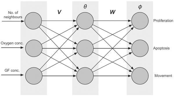
The layout of the intra-cellular response network which determines the behaviour of the cells. The mirco-environment of each cell is presented to the input layer of the network. This information is then fed through the network under the influence of the connection matrices V, W and the threshold vectors θ, φ, and the node with the strongest response in the output layer determines the behaviour of the cell. If no node reaches a value above 1/2 the cell becomes quiescent.

The value of the input layer is determined by the mirco-environment of the cell (i.e. one node for each of the three input variables; number of cell neighbours, oxygen and growth factor concentrations), these values are then fed through the network and produce a response in the output layer that determines the behaviour of the cell. In other words, if we let ξ = (n,c,g) represent the input to the network, then the value of node j in the hidden layer is given by

$$x_j=g\left(\sum _k{V}_{\mathit{jk}}{\xi }_k-{\theta }_j\right)$$

where $g\left(x\right)=\frac{1}{1+e^{-\beta x}}$ is a standard sigmoidal transfer function which guarantees that the node value is in the range [0,1]. The state of the nodes in the output layer is then given by

$$y_j=g\left(\sum _k{W}_{\mathit{jk}}{x}_k-{\varphi }_j\right).$$

Each node in the output layer corresponds to a phenotype or behaviour, and the node with the strongest response, and at least above 1/2, determines the action of the cell. If no node reaches above the value 1/2 the cell becomes quiescent and does nothing. For a more detailed description of the network dynamics and its implementation we refer the reader to (Gerlee and Anderson, 2009b).

2.1.2. Chemical fields

Cells forming a multicellular structure, such as the simple tissue architecture we consider, require a large number of different chemical compounds to promote and maintain growth and development. However, for the sake of simplicity we have limited ourselves to only one nutrient (oxygen) and one growth factor in our model. The reason for this choice is that they represent two different types of compounds from a biochemical perspective. Oxygen is a necessary compound for cell survival, as it plays a key role in metabolism, while GFs are necessary for cell division in most multicellular organisms. All cells are therefore assumed to consume oxygen, although at a different rate depending on their phenotype, while only proliferating cells take up GF. The compounds are further assumed to diffuse within the tissue, and therefore obey the following equations.

Oxygen equation

$$\frac{\partial c(\overrightarrow{x},t)}{\partial t}=D_c{\nabla }^{2}c(\overrightarrow{x},t)-f_c(\overrightarrow{x},t)$$ (1)

GF equation

$$\frac{\partial g(\overrightarrow{x},t)}{\partial t}=D_g{\nabla }^{2}g(\overrightarrow{x},t)-f_g(\overrightarrow{x},t)$$ (2)

where the GF consumption rate f_g(x,t) = k_g if the cell at position x is in a proliferating state and zero otherwise, while the oxygen consumption rate f_c is defined as

$$f_c(\overrightarrow{x},t)=\{\begin{array}{c}{k}_p,\text{if the cell at}\overrightarrow{x}\text{is proliferating}\hfill \\ k_m,\text{if the cell at}\overrightarrow{x}\text{is motile}\hfill \\ k_q,\text{if the cell at}\overrightarrow{x}\text{is quiescent}\hfill \\ 0,\text{otherwise}\hfill \end{array}\phantom{\}}$$

The production of oxygen and growth factor is assumed to take place on the domain boundary through diffusion from surrounding tissue or blood vessels, and is included by assuming Dirichlet boundary conditions with constant values, c₀ and g₀ respectively.

We will consider a thin slice of tissue, with M ⪡ N, and therefore assume that the concentration fields vary insignificantly in the z-direction, and thus only solve the equations (1) and (2) in two dimensions. This also implies that the boundary conditions are assumed to be constant along the z-direction. These equations are therefore discretised using a standard five-point finite central difference formula with space step Δx and time step Δt, and then solved using an implicit ADI-scheme (Press et al., 1996), which is iterated every time step of the simulation. The space step Δx is chosen such that it coincides with the cell size.

2.1.3. Cell behaviour

The behaviour of each cell depends on the dynamics of its response network, which in turn depends on the micro-environment in which it resides. In this section we will describe how the four possible phenotypes in the model, proliferative, motile, dead, and resting, are implemented.

2.1.3.1. Proliferative

For each time step a cell is in a proliferative state an internal counter is incremented and when it has reached a certain value t_p, corresponding to the time of the cell cycle, the cell divides and a daughter cell is placed at random in one of the neighbouring empty grid points (using a von Neumann neighbourhood). If no empty space exists cell division is halted until empty space emerges.

2.1.3.2. Motile

If a cell takes on the motile phenotype it moves at random into one of the empty neighbouring grid points. If no empty space exists the cell remains stationary. In order to modulate the velocity at which cell movement occurs, a cell in the motile state only moves with a given probability p_m.

2.1.3.3. Dead

If apoptosis is the response from the network, then the cell dies through controlled cell death, which means that it is rapidly broken down and the cell material is taken up by nearby cells. In the model this is implemented by letting the grid point where the cell resided become empty in the following time step. A cell can also die from starvation or necrosis which occurs when the oxygen concentration falls below a given threshold c_n. In order to account for the stochastic nature of cell behaviour we also include a small spontaneous death rate p_d, which is the rate at which cells die independent of the response from the network.

2.1.3.4. Resting

Finally, if none of the nodes in the output layer of the response network reach a value above 1/2 the cell remains passive in a quiescent state. Note that in this inactive state the cell consumes oxygen at lower rate than when proliferating or moving.

2.1.4. Cellular automaton

The initial conditions of the system are uniform concentrations of oxygen and GF, both at background levels (c₀ and g₀), and a single cell with a given genotype (set of network parameters) at the centre of the bottom layer, i.e. position x = (N/2,N/2,1). At the start of each time step the chemical concentrations are solved using the discretised equations. The position of each cell is then corrected with respect to neighbouring cells that have moved or died. This is done in order to avoid having cells suspended above the tissue, and simply means that we let a suspended cell drop along the z-axis (pulled by gravitation) until it touches another cell or the bottom of the domain. All the cells on the grid are then updated in a random order as follows:

1. The micro-environment $\left(n\right(\overrightarrow{x},t),c(\overrightarrow{x},t),g(\overrightarrow{x},t\left)\right)$ is sampled and the the intra-cellular response of network is calculated

2. The cell consumes oxygen and GF according to the phenotype chosen

3. The actions associated with the chosen phenotype are carried out and the grid is updated accordingly

The boundary conditions for the cells are reflective, i.e. the boundary presents an obstacle which the cells include when they sense the number of neighbours. This is meant to imitate a situation where a tissue develops within a bounded domain.

2.2. Parameters

As we are interested in the evolution of cell behaviours that can maintain tissue homeostasis we do not specify any parameters related to the response network. This means that we leave the network parameters undefined, and will instead let them emerge from the evolutionary algorithm (discussed below). In order to make the space of possible solutions smaller, and to fulfill biochemical constraints we will specify the cellular consumption rates of oxygen and GF.

Cancer cells growing in multicellular spheroids are known to consume oxygen at a rate 4.5 × 10⁻¹⁷ mol cell⁻¹ s⁻¹ (Freyer et al., 1984), and we therefore set the consumption rate of proliferating cells to k_p equal to this value. We assume that motile cells consume oxygen at a lower rate k_m = k_p/2, and that quiescent cells have an even lower consumption rate k_q = k_p/5, both within the experimentally determined range (Freyer et al., 1984). The consumption rate of GF is more difficult to estimate as it depends on the type of GF and cell type considered, we set it to k_g = 5.2 × 0⁻²⁴ mol cell⁻¹ s⁻¹, similar to the value used in Chang et al. (2000).

The time for the cell cycle also depends on the cell type under consideration, and we set it to the average value of endothelial cells t_p = 16 h (Calabresi and Schein, 1993). The background concentrations are set to c₀ = 0.28 mM = 0.28 × 10⁻⁶ mol cm⁻³ (Casciari et al. 1992) and g₀ = 10⁻¹³ mol cm⁻³ (Anderson and Chaplain, 1998). The concentration below which cells die from starvation is variable, we set it to be 1% of the background oxygen concentration (Anderson, 2005). The diffusion constant of oxygen in tissue is D_c = 1.8 × 10⁻⁵ cm² s⁻¹ (Waddington, 1959; Grote et al., 1977), and the diffusion constant of FGF8 (a typical growth factor) has been experimentally determined to D_g = 2 × 10⁻⁹ cm² s⁻¹ (Poplawski et al., 2007). The rate at which cells spontaneously go into apoptosis is difficult to estimate, we used the small value p_d = 10⁻³ cell⁻¹ cell cycle⁻¹. The movement probability was set to p_m = 0.5, which means that an uninterrupted motile cell will move at an average speed of 8 × 10⁻⁶ cm s⁻¹, similar to the value measured by Zaman et al. (2006).

The size of the grid was set to N = 200 and M = 8, meaning that we simulate a thin tissue architecture, which can at most contain 320,000 cells. Finally, the grid constant was set to Δx = 10 μm and the time step to Δt = 1.6 h, one tenth of the cell cycle time. Therefore our slice of tissue measures 2 mm × 2 mm × 0.8 mm.

2.3. Genetic algorithm

Evolutionary approaches have been used to solve various problems in computer science, such as hardware development, image classification and robot control (Banzhaf et al., 1997). What these approaches all have in common is that they try to harness the power of natural selection when solving the problem in question. Central to this is the notion of a fitness function, which to each candidate solution assigns a value, allowing us to rank all the solutions to the problem. Another necessary feature is that the solutions can be randomly modified (mutated) and even mixed with each other.

In our case, the problem is to find a set of network parameters or genotype, which when seeded into a single cell, and given time to grow, give rise to a tissue which is homeostatic. More precisely we want the single cell to multiply so that the population creates a mono-layer of cells at the bottom of the grid, such that no cells are stacked on top of each other, and maintains this structure over time. In order to asses this capability we would optimally track the tissue structure over an extended period of time, but due to computational constraints we settle for a single time-point measurement, and then in the smaller set of candidate solutions perform an exhaustive check for homeostatic behaviour. The simplified fitness function used in the EA is therefore

$$F=\stackrel{F_1}{\overbrace{\text{no. of cells in the bottom layer}}}+\stackrel{F_2}{\overbrace{\text{no. of empty grid points in all other layers}}}$$ (3)

measured at a single time-point. The goal is then to find a network architecture (i.e. genotype) which when distributed across the many cells forming the tissue maximises this function. In order to calculate the fitness of any given genotype an entire simulation with the hybrid cellular automaton model is necessary, and the number of time steps t_max in the simulation should be sufficient to allow the cell population to fill the entire domain and to test for its homeostatic capabilities. Naturally a very large t_max would be optimal, but this would be computationally expensive.

Another complication is that the fitness function is multiobjective, i.e. it contains two distinct parts, and in this case it has been shown that simply summing the two is not the best approach (Bentley and Wakefield, 1998). Instead we employ the sum of weighted ratios (SWR), which assigns weights to the different objectives depending on the current minimum and maximum values of the two objectives in the population. If we call the two objectives F₁ and F₂, then the fitness of genotype g is defined as

$$F\left(g\right)=\frac{F_1\left(g\right)-F_1^{\min }}{F_1^{\max }-F_1^{\min }}+\frac{F_2\left(g\right)-F_2^{\min }}{F_2^{\max }-F_2^{\min }}$$ (4)

where $F_i^{\min ,\max }$ refers to the minimum and maximum value of each objective currently present in the population. Please note that the use of this type of normalised fitness function implies that neither the average nor the maximum fitness (equation (3)) necessarily increases over time, the reason being that normalised fitness function prioritises the objective with the largest variation, which might lead to a drop in the overall fitness.

The evolutionary algorithm consists of a population of candidate solutions, which are subject to a selection process, where each individual in the population represents a given network architecture. We have chosen a tournament based selection process, which also makes use of a low degree of elitism. This means that a fraction (p_e = 5%) of the best solutions are carried unaltered into the next generation, while the rest of the EA-population engages in tournaments. Four solutions are picked at random and are compared in pairs, and this generates two winners and two losers. The winners are carried over to the next generation, while the losers are replaced by the offspring of the winners. The offspring are either generated by single point mutations to the parent's genotypes (occurs with probability 1/2) or by crossing-over their two genotypes (with complementary probability 1/2). This process is repeated until all solutions in the population have engaged in a tournament, and this constitutes one generation in the evolutionary algorithm. See Fig. 2 for a graphical representation of the selection process.

Fig. 2.

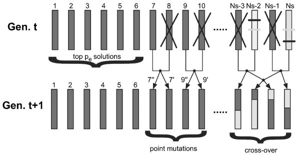
Schematic of the evolutionary algorithm. In each generation the top p_e most fit solution are carried unaltered into the next generation. The remaining genotypes are paired off in tournaments where the winners give rise to offspring either by point mutations or cross-over.

The point mutations are implemented by changing one of the network parameters (matrix entries or node thresholds) into a random number chosen from a normal distribution. The cross-over is implemented by mapping the network parameters of both parents into two vectors, picking two random indices and swapping the contents above and below these points. In most cases this is disruptive, but in some cases it generates a novel solution with a higher fitness than the parents.

Each run was started with an EA-population of size N_s = 50, where all genotypes were randomly generated. The number of time steps used for each fitness evaluation was t_max = 200, which since the size of the grid is 200 × 200, means that a genotype with proliferative capabilities will be able to fill the entire domain, whilst still needing to exhibit homeostatic behaviour to receive a high fitness (if the cells at the edge of the growing tissue are constantly dividing the domain boundary will be reached in approximately 100 cell cycles). The total number of generations iterated with the EA was set to T_max = 20, which means that we had to run N_s + (1 − p_e)N_sT_max/2 = 500 realisations of the underlying hybrid cellular automaton model.

This procedure is very CPU-intensive, as we need to run the CA for 200 time steps each time a new individual is generated. This is especially wasteful in the early generations when many solutions are poor. In order to reduce computational time we therefore implemented another scheme for fitness evaluation, which is incremental. This means that at the beginning of the EA-run we set the simulation time used for fitness evaluation to t_max = 20 (the simulation time within the CA), and then increase it in steps of 20 time steps every 5 EA-generations. When an evaluation time of 200 time steps is reached at generation 48 we continue the EA with this fixed evaluation time for another 20 generations. Using this method we can evaluate more generations in shorter CPU-time, but it also has the side-effect that we are selecting for genotypes which give rise to fast-growing tissues, as those which are able to spread fast will be assigned a larger fitness (the first term in equation (3) will be larger). In the following sections we will refer to the former method as a fixed fitness evaluation, and the latter as the incremental method.

For the sake of clarity we would like to remind the reader that the system we are dealing with contains two distinct levels: the evolutionary algorithm (EA) which contains a population of candidate solutions, and the hybrid cellular automaton (HCA) model which describes the growth of a tissue consisting of a population of cells. Each solution in the EA consists of a network architecture encoded in a genotype, which prescribes the behaviour of the cells in HCA. We are selecting for homeostasis within the HCA, and to achieve this we make of use of an EA.

3. Results

Because the EA is seeded with a population of random network architectures, and only random variation and selection drives the search for a homeostatic genotype, the only constraint that we impose on the solution is that of the network representation of the genotype to phenotype mapping. Our aim was to study evolutionary plausible mechanisms for homeostasis in our CA model.

The results of a typical run of the EA (with fixed evaluation) are displayed in Fig. 3. Panel (a) shows the growth patterns generated by the fittest genotype in each generation of the run. What is shown is the distribution of cells in the domain at the end of each fitness evaluation, i.e. at t_max = 200 time steps (cell cycles), from a top view (if several cells are stacked on each other only the topmost cell is visible).

Fig. 3.

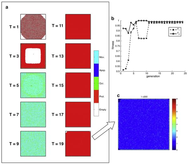
Time evolution of the EA. (a) shows the tissue structure formed by the most fit genotypes at different generations in the run. Here proliferating cells are shown in red, motile cells in cyan and quiescent cells in green. The time evolution of the average normalised fitness for the two objectives is shown in (b), which because of SWA (equation (4)) does not necessarily increase over time. The cell density of the final genotype (T = 19) is shown in (c). Supplementary movie of the growth dynamics of the final genotype can be found at http://sysbio.med.gu.se/gerlee/homeostasis.html.

From this sequence we can see that the EA has explored several different solutions before settling on a completely proliferating genotype at T = 11–19. In the beginning of the run, at T = 1 the fittest solution is a genotype giving rise to a slow growing tissue with a low cell density. This is then replaced by a genotype, which forms a ring-like structure where no cells reside in the interior of the domain (T = 3). From T = 5 to 9 the fittest genotype is one which fills the entire bottom of the domain, and many of the cells are in a motile state. This type of solution is then taken over by one which relies fully on proliferation and which remains the most fit solution until the end of the run. The average normalised fitness split into the two contributions F₁ and F₂ (see equations (3) and (4)) for this run is shown in Fig. 3b. Here we observe that both fitness curves occasionally drop during the run, and the reason for this is that we make use of the SWR-fitness function (equation (4)), which trades off fitness gains in one objective for fitness losses in the other. In any case there is a clear improvement in fitness, particularly in the first component, from the most fit solution (genotype) at T = 1 to the most fit genotype at the end of the run which has a fitness approximately equal to one in both fitness components.

In order to get a better understanding of the tissue architecture generated by final genotype we also plotted the cell density in the domain at t = 200. This can be seen in Fig. 3c, and shows that most of the tissue consists of a mono-layer of cells with a few isolated cells lying on top (the mean cell density is 1.08 cells/bottom grid point). This means that the genotype producing this growth pattern meets the requirements of the fitness function fairly well, however, the information gathered thus far is insufficient to allow us to understand how this possibly homeostatic behaviour is achieved, but we will return to this later.

This illustration only shows one possible solution found by the EA, and in order to investigate the system more thoroughly we ran 20 instances of the EA for each fitness evaluation method, seeded with different random initial populations of solutions. Because of the simplified single time-point fitness function used in the EA, we had no guarantee that the EA would generate genotypes which could achieve mono-layer homeostasis, or homeostasis at any cell number. In order to test for this we ran the hybrid-CA with each of the 40 genotypes, and measured the cell count as a function of time in the span t = 200–400. If the cell count remained stable we classified the genotype as homeostatic. We found that 11 of the fixed EA-runs and 12 of the incremental runs gave rise to network architectures that exhibited homeostatic behaviour. The remaining solutions exhibited similar growth dynamics in the beginning of the simulation, but never reached homeostasis and kept on growing in cell number albeit at a low rate.

In our efforts to determine homeostatic capabilities we initially tried to lower the amount of CPU-time by skipping the developmental step and initialising the tissue as a mono-layer and starting the simulations from that point. This did however for many of the genotypes give a different non-homeostatic outcome compared to simulations starting with a single cell, suggesting a link between development and homeostasis in the model, which we will return to in the Discussion.

3.1. Analysis and testing of the homeostatic genotypes

The 11 (fixed) + 12 (incremental) = 33 genotypes that passed our test for homeostasis were kept and analysed further. Firstly we measured at what cell count they maintain homeostasis, and also the rate of cell turnover. As the tissue is homeostatic the net growth in cell number is zero, meaning that the rate of cell division is equal to the rate of cell death. Please note that because of the spontaneous death rate of p_d = 10⁻⁴ cell⁻¹ update⁻¹ the turnover is always non-zero. The results are shown in Fig. 4, and reveal a clear separation between the outcomes produced by the two types of fitness evaluation methods. The cell types obtained from the fixed evaluation method exhibit cell number close to the optimal of 200 × 200 = 40,000, and have a high rate of cell turnover, while the cell types that emerged from the incremental method produce a greater cell number, but with a considerably smaller rate of cell turnover (number of cell divisions per time step). In fact, both the total cell number and turnover rate are significantly different for the two evaluation methods (P < 10⁻² and 10⁻⁶ respectively in a paired sample t-test).

Fig. 4.

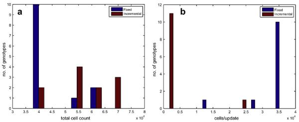
(a) The total cell count when the tissue has reached homeostasis and (b) the cell turnover rate during homeostasis. The general trend is that genotypes from the fixed scheme has a lower total cell count, but a higher cell turnover rate compared to the genotypes evolved in the incremental scheme.

The two evaluation methods clearly generate a range of network architectures that produce homeostatic tissue structures but differ significantly in their behaviour, and this begs the question of how this impacts their robustness to perturbations. Biological systems encounter many types of perturbations, to which they must be sufficiently robust, such that the system continues to function properly. Typically these are classed as external and internal fluctuations, and here we will focus on disruption in tissue structure, i.e. wounding, as external perturbations, and mutations to the genotype (i.e. the response network) as internal perturbations.

3.1.1. External perturbation: wounding

For our purposes wounding can be interpreted as either the removal of cells from the tissue (negative wounding) or the increase of local cell density from the addition of cells (positive wounding). The negative wounding is comparable to the physical removal of cells as in a laceration, while the positive could be compared to the increase in cell density induced by the growth of a tumour in the tissue.

The negative wounding experiments where carried out by first letting the genotypes form a homeostatic tissue, then removing all cells in a circle of radius 50, and measuring the time it took for the tissue to return to a homeostatic state. We also quantified how well healing was achieved by measuring the difference in cell count between the newly attained homeostatic state and the original. The positive wounding was performed in a similar way with the difference that the tissue was over-crowded by filling the entire computational domain with cells. A typical result of these experiments can be seen in Fig. 5, which shows how the tissue recovers from the perturbation and returns to homeostasis. Please note that the time-scale of healing is quite different for the two experiments, the negative wounding takes on the order of 10 cell generations to heal, while the positive only takes about one generation. The results from the fixed and incremental evaluation methods are summarised in Table 1, which shows the average (standard error in brackets) of the healing time for the positive (T+) and negative (T−) wounds and respective deviations (D+/−) from the original homeostatic populations.

Fig. 5.

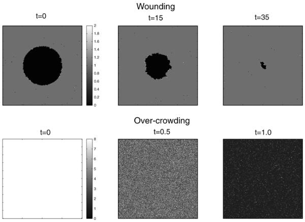
Typical example of wound healing. The upper panel shows the healing of a circular (negative) wound, and the lower shows the recovery from an over-crowding of the entire domain. Please note the difference in time-scale in the two processes. Supplementary movie of the recovery from wounding can be found at http://sysbio.med.gu.se/gerlee/homeostasis.html.

Table 1.

The average healing time and resulting population deviation for the evolved genotypes. The averages and standard errors were calculated for the two groups separately with 11 and 12 samples in each.

	T−	D−	T+	D+
Fixed	56 (0.9)	97 (58)	7 (0.5)	5230 (2023)
Incremental	47 (3.9)	629 (844)	45 (8)	158,490 (23,936)

3.1.2. Internal perturbation: mutation

The robustness to mutations was quantified by evaluating the fitness of each genotype when mutations are present within the hybrid cellular automaton. This means that the cells in the tissue are not necessarily mono-clonal (since mutations within a simulation of the HCA might generate mutants), and this variation in genotype can also lead to significant changes in cell behaviour (i.e. cell phenotype). Here we would like to differentiate between two different kinds of mutations that real cells receive, those that occur during cell division when DNA is being copied and those that occur at any time during the cell cycle. The latter kind is typically induced by mutagenic compounds or external factors such as cosmic rays. We therefore refer to this kind as `cosmic ray' mutations, while the former kind is simply called `copy' mutations. As before we allow the tissue to develop in the absence of perturbations, with the mutation rate set to zero, and then turn on mutations and run the simulation for 100 cell generations. At the end of the simulation we calculate the raw fitness F_m (using equation (3)), which is normalised into a relative fitness F_r = F_m/F₀ by dividing with the fitness achieved in the absence of mutations. How robust the genotypes are to these mutations do of course depend on the actual mutation rate, but since we are interested in the relative difference between the different genotypes the exact mutation rates are less important, provided they are in a biologically reasonable range. The copy mutation rate was set to 10⁻⁴ division⁻¹ and the cosmic ray mutation rate equaled 10⁻⁶ cell⁻¹ update⁻¹. The relative fitness under both kinds of mutations was averaged over 5 simulations and the results can be seen in Fig. 6. All genotypes obtained from the fixed evaluation are plotted in panel (a) and the incremental ones in panel (b). The general trend here is that genotypes evolved in the fixed evaluation scheme do worse under copy mutations, while the reverse seems to be true for the incremental ones (except for one outlier) although the trend is weaker.

Fig. 6.

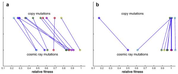
Comparison between the robustness to `copy' and `cosmic ray' mutations'. Colours reflect distinct genotypes and connections highlight how fitness changes under each type of mutation. (a) shows the genotypes from the fixed fitness evaluation scheme while (b) the ones from the incremental scheme.

The results presented thus far point to a difference between the genotypes (and resulting cell phenotypes) evolved in the fixed and incremental fitness evaluation schemes. The first clue to this is that the turnover rate for the cells from the fixed class are considerably higher. In fact if we calculate the fraction of cells that are replaced every cell generation we see that on average 83% of all the cells in the tissue are replaced every cell cycle, while the corresponding value for the cells from the incremental class is approximately 0.5%. This suggests two very different mechanisms for maintaining homeostasis, which we now examine by looking in detail at how the cells from the two classes phenotypically behave.

3.2. Mapping micro-environment to cell phenotype

A useful way of analysing the behaviour of a given network architecture or genotype is to calculate its corresponding cell phenotype in all possible micro-environmental conditions. As the input to the intra-cellular network is 3-dimensional (no. of neighbours, oxygen and GF concentration) and the output is 1-dimensional and discrete (proliferation, movement, apoptosis and quiescence), the behaviour of the genotype can be visualised as a function from 3 to 1 dimensions, where each point in the output space is associated with a behaviour (cell division, movement, death and quiescence). An example of this type of phenotype map was generated for a cell from a run with fixed evaluation and is shown in Fig. 7a. From this figure we can conclude that the behaviours resulting from this genotype are limited to proliferation and apoptosis. The lack of any quiescence or movement in this apparently homeostatic genotype suggests that apoptosis might play an important role in its behaviour. This absence of quiescence was seen in all of the phenotype maps generated from genotypes produced using the fixed evaluation function. If we on the other hand analyse the behaviour of a genotype from the incremental class (Fig. 7b) we see that it also consists mostly of proliferation and apoptosis, but that there is a small (but obviously significant) subset of the input space which gives rise to motility. This motility region was observed in the phenotype maps produced from all except one of the incremental class genotypes (the outlier in Fig. 6b).

Fig. 7.

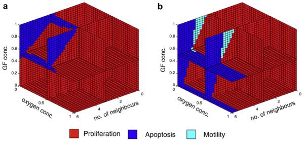
The behaviour of two network architectures (genotypes), one from each class (fixed and incremental), visualised by mapping each point in the micro-environmental input space to the associated behaviour determined by the response network. Here proliferation is shown in red, apoptosis in blue, and motility in cyan.

Viewing these mappings from environmental input to cell behaviour, in the context of tissue structure can explain these differences. The networks obtained from the fixed evaluation (Fig. 7a) will give rise to cell division when placed in a mono-layer (i.e. has 4 neighbours). There will however be no space for the daughter cells within the mono-layer, and they will instead be placed on top of the existing cells in a new layer. Now the cells in the bottom layer will sense a higher cell density (no. of neighbours), and this causes them to go into apoptosis. This frees up space, and the daughter cells will drop down to the bottom layer of the grid returning the tissue to its mono-layer structure. Whilst this behaviour does not occur in the simulation in such a synchronized manner, the average cell turnover rate is still considerable. In contrast, the networks evolved with the incremental evaluation scheme (Fig. 7b) can maintain a mono-layer of cells, as it becomes motile (or essentially quiescent due to insufficient space to move) when it has 4 neighbouring cells (assuming sufficient GF is present). Only when it encounters a hole in the mono-layer, which corresponds to a local cell density of 3 cells, does it go into proliferation. This statement is clearly not true for all the cell types in the incremental class, as most of them exhibit a cell number well above the 40,000 which corresponds to a true mono-layer, but the low turnover rate reveals that they are far more conservative in their mechanism for maintaining homeostasis than the fixed class.

4. Discussion

We have shown that by coupling a hybrid cellular automaton model of tissue growth, where the behaviour of each cell is determined by an intra-cellular signalling network, with an evolutionary algorithm we could evolve genotypes which form a homeostatic tissue. In the EA we used two different schemes for fitness evaluation, one with a fixed simulation time of 200 cell cycles, and one with an increasing simulation time that eventually achieves 200 cell cycles.

These two variants of the EA gave rise to network architectures which fell into two classes with respect to their behaviour. The solutions emerging from the fixed evaluation where characterised by cell numbers close to the optimum and high turnover rates, which we consider as wasteful, while the solutions from the incremental setting gave rise to sub-optimal solutions that nevertheless had much lower cell turnover rates, which we label as conservative.

The evolved networks were characterised by measuring how they respond to external and internal perturbations. In these experiments the two classes were clearly separated, suggesting that the mechanism by which a tissue remains homeostatic has implications for its robustness. In the wounding experiments it was found that the genotypes from the fixed evaluation form tissues which heal faster and more accurately, except for the healing time of the circular wound, which was slightly lower for the conservative genotypes. The latter type was however particularly bad at returning to the same cell count prior to the wounding. This points to the fact that the homeostatic mechanism itself was affected by the perturbation, suggesting a lower degree of robustness in this tissue structure.

In the mutation experiments we found that the wasteful genotypes do worse in an environment dominated by copy mutations as compared to cosmic ray mutations, while the opposite was found for the conservative genotypes. The explanation for this can be found in the way homeostasis is achieved. The wasteful genotype is prone to accumulate mutations, which occur during cell division because of the elevated cell division rate. On the other hand, because it sheds cells at a high rate this could be an advantage in an environment where the rate of spontaneous mutations is high, as the cells will not have time to accumulate many mutations before they go into apoptosis. The conservative genotype is on the contrary better suited to a situation where the mutation rate during replication is high, while the spontaneous mutation rate is low.

The two classes of evolved genotypes present contrasting mechanisms by which tissue homeostasis can be maintained. One does so by continually shedding cells by apoptosis, the other by lowering the total proliferation rate of the tissue so that it just balances the spontaneous rate of cell death. One could argue that the proliferative genotype maintains homeostasis in a wasteful manner by continually replacing the cells in the tissue, but as we did not include any notion of resourcefulness in the fitness function one should not be surprised at this type of solution. This could however be enforced by reducing the background oxygen or GF concentration to levels which could not sustain constant tissue renewal.

This separation into two classes compares well to different homeostatic tissue types found in multicellular organisms. For example the epithelial cells lining the colon in humans are shed at a considerable rate (Podolsky and Babyatsky, 2003). These cells are exposed to a hostile environment where the rate of spontaneous mutation is elevated, and in order to avoid harmful mutations accumulating in these cells they are continually removed. Similar tissue architecture is found in the outer layers of the skin, where cells also have a short life span. In other tissue types, which are not as exposed, the opposite type of homeostatic mechanism is normally found, i.e. only when cells die spontaneously are they replaced (Hooper, 1956).

Our hypothesis is that both homeostatic mechanisms could coexist in the same organism. Different tissues in the same organism have different requirements and constraints and thus could have evolved different schemes. A genotype giving rise to a proliferative cell behaviour is more likely to evolve in an environment where the rate of spontaneous mutations is high, while a conservative behaviour is likely to evolve when the mutation rate during cell division is elevated.

In our model the two mechanisms did however not evolve, as is most likely in the above cases, due to the selection pressure imposed by different environments. The only difference between the two selection schemes in this study was the variation in evaluation time (fixed vs. incremental), and this must explain the observed difference. A by-product of the incremental scheme is that in the early stages of the EA, when the evaluation time is small, we also select for fast-growing genotypes, as these attain a higher fitness (see equation (3)). Fast growth is most easily achieved by a tissue, which expands not only by proliferation but also by motility. The motile cell phenotype does however, due to the specifics of our model, turn into a quiescent resting cell, when no free space to move into exists. This fact is exploited by the fast-growing genotypes as an easy route to achieve homeostasis in a conservative fashion. When no incentive for growing fast exists the EA instead converges on solutions, which are dominated by proliferation and apoptosis. This is at least in part due to the model assumptions: (i) there is no obvious cost for proliferation and (ii) no mutations occur during fitness evaluation. The former neglects the metabolic needs of a tissue with a high cell turnover, and the latter is akin to the assumption that mutations always occur in the germ line but never in somatic cells. If these two features where amended in the model the difference between the two schemes would probably lessen.

Another feature of the model, which also deviates from what we find in real organisms, is that the GF, which is consumed by the proliferating cells, and has the possibility to influence cell phenotype through the response network, does not play an active role in regulating cell behaviour. From Fig. 7 it might seem that the GF concentration influences behaviour, but in fact during simulation the GF concentration in the entire domain is almost constant. Instead the cells rely on cell–cell communication (i.e. no. of neighbours) to dictate their behaviour. The number of neighbours a cell has is simply a more informative measure than the local GF concentration when mono-layer homeostasis is the objective. However, when more complicated architectures are selected for, that for example require positional information, a gradient of GF might prove useful and even necessary (Wolpert, 2007).

Although the mono-layer structure we selected for is a comparatively simple tissue architecture we still found a developmental dependence which could not be circumvented. If the hybrid cellular automaton was initialised in a mono-layer state with oxygen and GF at background concentrations we observed that some genotypes did not behave homeostatically, but kept on increasing in cell number. The difference between this set-up and one which has gone through the developmental process of growing into a mono-layer is the concentration profiles of oxygen and GF, which have not changed in step with the developing tissue, but instead exhibit a uniform distribution. This shows that the dynamics of the tissue are contingent on the developmental process (Waddington, 1959), and might be shifted to a different mode by perturbing the environment.

The resulting tissue structure, which is what we selected for, emerges from the genotype in a complex non-linear fashion, and to predict what type of tissue a certain network structure or genotype gives rise to is difficult without resorting to simulation. In our model we can identify three levels of organisation: genotype/network, cell phenotype and tissue structure, while in real organisms the levels of organisation are much larger in number and sometimes difficult to separate. Understanding how organisms emerge from genotypes, i.e. how the genotype–phenotype (GP) map is structured (Pigliucci, 2010), is a central problem in biology and embryology. This map has typically been studied in simple systems, such as RNA-folding (Fontana and Schuster, 1998) or protein function (Wroe et al., 2007), but by considering more complex systems that incorporate a dynamic developmental process and importantly in an evolutionary context we hope to increase the understanding of the relation between genotype and phenotype.

By considering the GP-map in an evolutionary context we go one step further, thus circumventing a critical problem with these approaches – which is how to define the mapping in the first place. Utilizing the EA to parameterise the network is a novel technique to create multiple unbiased developmentally sound genotypes that could have many other applications. Critically this approach naturally unifies the gene-centric and environment-centric views of development i.e. it is both preprogrammed and emergent, the genotype gives the cells the ability and the interactions and microenvironment allow the cell to realize them with a range of phenotypes.

The model presented in this paper is clearly a caricature of how the development of real tissue unfolds and how it is maintained. In order to make the model feasible, and understandable, we have made gross simplifications to both the intra- and extra-cellular dynamics. The response network is an abstraction of the immensely complex gene regulatory network of real organisms, and we have ignored many chemical and mechanical cues mediating cell–cell communication.

Here we have deliberately circumvented the incredible complexity of the true dynamics, in favour of a functional analogy that still allows us to understand key principles underlying our multi-scale system.

With a better charaterisation of how healthy tissue functions and is maintained we will hopefully be able to turn to the question of how diseases such as cancer and autoimmune diseases are initiated and progress and critically how they might be cured. Using evolved genotypes that develop into normal tissue we can investigate which genetic and external perturbations lead to a disease-state, and investigate how this process can be halted or even reversed.

References

- Andersen T, Newman R, Otter T. Shape homeostasis in virtual embryos. Artif. Life. 2009;15(2):1–23. doi: 10.1162/artl.2009.15.2.15201. [DOI] [PubMed] [Google Scholar]
- Anderson ARA, Chaplain MAJ. Continuous and discrete mathematical models of tumor-induced angiogenesis. Bull. Math. Biol. 1998;6:857–899. doi: 10.1006/bulm.1998.0042. [DOI] [PubMed] [Google Scholar]
- Anderson ARA. A hybrid mathematical model of solid tumour invasion: the importance of cell adhesion. Math. Med. Biol. 2005;22:163–186. doi: 10.1093/imammb/dqi005. [DOI] [PubMed] [Google Scholar]
- Banzhaf W, et al. Genetic Programming: An Introduction. Morgan Kaufmann Publishers; 1997. [Google Scholar]
- Basanta D, Miodownik M, Baum B. The evolution of robust development and homeostasis in artificial organisms. PLoS Comput. Biol. 2008;4(3):e1000030. doi: 10.1371/journal.pcbi.1000030. [DOI] [PMC free article] [PubMed] [Google Scholar]
- Bentley PJ, Wakefield JP. Soft Computing in Engineering Design and Manufacturing. Springer-Verlag; 1998. Finding acceptable solutions in the pareto-optimal range using multiobjective genetic algorithms; pp. 231–240. [Google Scholar]
- Calabresi P, Schein PS. Medical Oncology. McGraw-Hill; NY: 1993. [Google Scholar]
- Camazine S, et al. Self-organisation in Biological Systems. Princeton University Press; 2001. [Google Scholar]
- Casciari JJ, Sotirchos SV, Sutherland RM. Variation in tumour cell growth rates and metabolism with oxygen-concentration, glucose-concentration and extra-cellular pH. J. Cell. Physiol. 1992;151:386–394. doi: 10.1002/jcp.1041510220. [DOI] [PubMed] [Google Scholar]
- Chang YS, et al. Mosaic blood vessels in tumors: frequency of cancer cells in contact with flowing blood. Proc. Natl. Acad. Sci. U S A. 2000:14608–14613. doi: 10.1073/pnas.97.26.14608. [DOI] [PMC free article] [PubMed] [Google Scholar]
- Chavoya A, Duthen Y. GECCO '06. ACM. 2006. Using a genetic algorithm to evolve cellular automata for 2D/3D computational development. [Google Scholar]
- Cunliffe J. Morphostasis: an evolving perspective. Med. Hypotheses. 1997;49(6):449–459. doi: 10.1016/s0306-9877(97)90062-1. [DOI] [PubMed] [Google Scholar]
- Fontana W, Schuster P. Continuity in evolution: on the nature of transitions. Science. 1998;280(5368):1451–1455. doi: 10.1126/science.280.5368.1451. [DOI] [PubMed] [Google Scholar]
- Freyer JP, et al. In situ consumption rates of cells in v-79 multicellular spheroids during growth. J. Cell. Physiol. 1984;118:53–61. doi: 10.1002/jcp.1041180111. [DOI] [PubMed] [Google Scholar]
- Gerlee P, Anderson A. A hybrid cellular automaton model of clonal evolution in cancer: the emergence of the glycolytic phenotype. J. Theor. Biol. 2007a;250:705–722. doi: 10.1016/j.jtbi.2007.10.038. [DOI] [PMC free article] [PubMed] [Google Scholar]
- Gerlee P, Anderson A. An evolutionary hybrid cellular automaton model of solid tumour growth. J. Theor. Biol. 2007b;246(4):583–603. doi: 10.1016/j.jtbi.2007.01.027. [DOI] [PMC free article] [PubMed] [Google Scholar]
- Gerlee P, Anderson ARA. Evolution of cell motility in an individual-based model of tumour growth. J. Theor. Biol. 2009a;259:67–83. doi: 10.1016/j.jtbi.2009.03.005. [DOI] [PMC free article] [PubMed] [Google Scholar]
- Gerlee P, Anderson ARA. Modelling evolutionary cell behaviour using neural networks: application to tumour growth. Biosystems. 2009b;95:166–174. doi: 10.1016/j.biosystems.2008.10.007. [DOI] [PMC free article] [PubMed] [Google Scholar]
- Greider CW, Blackburn EH. A telomeric sequence in the RNA of Tetrahymena telomerase required for telomere repeat synthesis. Nature. 1989;337(6205):331–337. doi: 10.1038/337331a0. [DOI] [PubMed] [Google Scholar]
- Grote J, Susskind R, Vaupel P. Oxygen diffusivity in tumor tissue (DS-carcinosarcoma) under temperature conditions within the range of 20–40 degrees C. Pflugers Arch. 1977;372:37–42. doi: 10.1007/BF00582204. [DOI] [PubMed] [Google Scholar]
- Hanahan D, Weinberg RA. The hallmarks of cancer. Cel. 2000;100(1):57–70. doi: 10.1016/s0092-8674(00)81683-9. [DOI] [PubMed] [Google Scholar]
- Hooper CES. Cell turnover in epithelial populations. J. Histochem. Cytochem. 1956;4(6):531–540. doi: 10.1177/4.6.531. [DOI] [PubMed] [Google Scholar]
- Kaneko K. Evolution of robustness to noise and mutation in gene expression dynamics. PLoS One. 2007;2(5):e434. doi: 10.1371/journal.pone.0000434. [DOI] [PMC free article] [PubMed] [Google Scholar]
- Nusslein-Volhard C, Wieschaus E. Mutations affecting segment number and polarity in drosophila. Nature. 1980;287(5785):795–801. doi: 10.1038/287795a0. [DOI] [PubMed] [Google Scholar]
- Pigliucci M. Genotype–phenotype mapping and the end of the `genes as blueprint' metaphor. Phil. Trans. Royal Soc. B. Biol. Sci. 2010;365(1540):557–566. doi: 10.1098/rstb.2009.0241. [DOI] [PMC free article] [PubMed] [Google Scholar]
- Podolsky DK, Babyatsky MW. Textbook of Gastroenterology. Lippincott; Philadelphia, PA: 2003. [Google Scholar]
- Poplawski NJ, et al. Adhesion between cells, diffusion of growth factors, and elasticity of the AER produce the paddle shape of the chick limb. Physica A. 2007;373:521–532. doi: 10.1016/j.physa.2006.05.028. [DOI] [PMC free article] [PubMed] [Google Scholar]
- Press WH, et al. Numerical Recipes in C: The Art of Scientific Computing. Cambridge University; 1996. [Google Scholar]
- Queitsch C, Sangster TA, Lindquist S. Hsp90 as a capacitor of phenotypic variation. Nature. 2002;417(6889):618–624. doi: 10.1038/nature749. [DOI] [PubMed] [Google Scholar]
- Rejniak KA, Anderson AR. A computational study of the development of epithelial acini: II. Necessary conditions for structure and lumen stability. Bull. Math. Biol. 2008a;70(5):1450–1479. doi: 10.1007/s11538-008-9308-3. [DOI] [PMC free article] [PubMed] [Google Scholar]
- Rejniak KA, Anderson AR. A computational study of the development of epithelial acini: I. Sufficient conditions for the formation of a hollow structure. Bull. Math. Biol. 2008b;70(3):677–712. doi: 10.1007/s11538-007-9274-1. [DOI] [PMC free article] [PubMed] [Google Scholar]
- Shaanker RU, Ganeshaiah KN, Krishnamurthy KS. Development of seeds as self-organizing units: testing the predictions. Int. J. Plant Sci. 1995:650–657. [Google Scholar]
- Shapiro BL. Down syndrome–a disruption of homeostasis. Am. J. Med. Genet. 1983;14(2):241–269. doi: 10.1002/ajmg.1320140206. [DOI] [PubMed] [Google Scholar]
- Spradling AC, Zheng Y. Developmental biology. The mother of all stem cells? Science. 2007;315(5811):469–470. doi: 10.1126/science.1138237. [DOI] [PubMed] [Google Scholar]
- Stanley KO, Miikkulainen R. A taxonomy for artificial embryogeny. Artif. Life. 2003;9(2):93–130. doi: 10.1162/106454603322221487. [DOI] [PubMed] [Google Scholar]
- Streichert F, et al. Evolving the ability of limited growth and self-repair for artificial embryos. Lect. Notes Artif. Int. 2003;2801:289–298. [Google Scholar]
- Sumedha, Martin O, Wagner A. New structural variation in evolutionary searches of RNA neutral networks. Biosystems. 2007;90:475–485. doi: 10.1016/j.biosystems.2006.11.007. [DOI] [PubMed] [Google Scholar]
- Thompson DAW. On Growth and Form: the Complete Revised Edition. Dover Publications; 1992. [Google Scholar]
- Turing AM. Morphogenesis. Collected Works of A. M. Turing. North-Holland, Amsterdam, The Netherlands: 1992. [Google Scholar]
- Waddington CH. The Strategy of the Genes. Macmillan; New York: 1959. [Google Scholar]
- Wagner A. Robustness and evolvability: a paradox resolved. Proc. R. Soc. B Biol. Sci. 2008;275(1630):91. doi: 10.1098/rspb.2007.1137. [DOI] [PMC free article] [PubMed] [Google Scholar]
- Wolpert L. Positional information and the spatial pattern of cellular differentiation. J. Theor. Biol. 1969;25(1):1–47. doi: 10.1016/s0022-5193(69)80016-0. [DOI] [PubMed] [Google Scholar]
- Wolpert L. Principles of Development. Oxford University Press; Oxford: 2007. [Google Scholar]
- Wroe R, Chan HS, Bornberg-Bauer E. A structural model of latent evolutionary potentials underlying neutral networks in proteins. HFSP J. 2007;1(1):79–87. doi: 10.2976/1.2739116. [DOI] [PMC free article] [PubMed] [Google Scholar]
- Zaman MH, et al. Migration of tumor cells in 3D matrices is governed by matrix stiffness along with cell-matrix adhesion and proteolysis. Proc. Natl. Acad. Sci. U S A. 2006;103:10889–10894. doi: 10.1073/pnas.0604460103. [DOI] [PMC free article] [PubMed] [Google Scholar]