A Computational Study of the Development of Epithelial Acini: I. Sufficient Conditions for the Formation of a Hollow Structure

Abstract

Normal hollow epithelial acini are 3-dimensional culture structures that resemble the architecture and functions of normal breast glands and lobules. This experimental model enables in vitro investigations of genotypic and molecular abnormalities associated with epithelial cancers. However, the way in which the acinar structure is formed is not yet completely understood. Gaining more information about consecutive stages of acini development—starting from a single cell that gives rise to a cluster of randomly oriented cells, followed by cell differentiation that leads to a layer of polarised cells enclosing the hollow lumen—will provide insight into the transformations of eukaryotic cells that are necessary for their successful arrangement into an epithelium. In this paper, we introduce a two-dimensional single-cell-based model representing the cross section of a typical acinus. Using this model, we investigate mechanisms that lead to the unpolarised cell growth, cell polarisation, stabilisation of the acinar structure and maintenance of the hollow lumen and discuss the sufficient conditions for each stage of acinar formation. In the follow-up paper (Rejniak and Anderson, A computational study of the development of epithelial acini. II. Necessary conditions for structure and lumen stability), we investigate what morphological changes are observable in the growing acini when some assumptions of this model are relaxed.

1. Introduction

Epithelial tissues line all cavities and free surfaces of the body and form highly selective barriers between different body compartments. Normal simple epithelia form one layered sheets of tightly packed cells that are surrounded by the supporting basement membrane. All processes of normal epithelial cells are tightly controlled and coordinated to ensure tissue integrity that is necessary for proper cell proliferation, survival, differentiation and enzyme secretion. Epithelial cells develop specialised cell–cell connections with their neighbours, such as adherens junctions that mechanically attach cells to one another, tight junctions that seal cells together to prevent leakage of molecules from one side of the epithelial sheet to the other, or gap junctions and chemical synapses that mediate the passage of chemical and electrical signals between neighbouring cells and provide a mechanism for coordinating the activities of individual cells in tissues. Similarly, the epithelial cells develop specialised connections that provide a mechanical attachment to the basement membrane and mediate exchange of signals with the extracellular matrix. All epithelial cells maintain an apical-basal polarity that is synchronised among all cells in the epithelium. In general, cell polarity is defined as asymmetry in cell shape, protein distribution and cell function (Nelson, 2003). In a multicellular tissue, however, the asymmetry of individual cells must conform to the overlying architecture of the tissue. In the epithelial cells, this is manifested by acquiring three different kinds of membrane domains: an unbounded apical side facing a free space enclosed by the epithelium (lumen), a bounded basal side that is in a direct contact with the extracellular matrix and one or more bounded lateral sides contacting the membranes of other cells (Nelson, 2003; O'Brien et al., 2002). In proliferating epithelial cells, the orientation of cell mitosis is controlled in such a manner as to maintain the normal tissue architecture and structural integrity. It has been observed that normal epithelial breast cells can acquire two specific orientations of the nuclear spindle, and thus two planes of cytokinesis. Cell division perpendicular to the lumen results in two luminally positioned daughter cells and leads to the duct outgrowth. Cell division parallel to the lumen, on the other hand, gives rise to one luminally and one basally positioned daughter cell, and culminates in the basal cell differentiation or its death by apoptosis (Ferguson and Anderson, 1981; Ferguson, 1985, 1988). Cell apoptotic death is a multi-step and multi-pathway process in which cells die without harming other cells in their environment. It occurs either as a result of some failure in the internal cell machinery, such as during DNA replication or in response to some external cues sensed via the death receptors located on the cell membrane. This process of cell death is very common during the normal embryonic development or normal tissue turnover. Cells dying by apoptosis detach themselves from their neighbours and the substrata. Their volume shrinks and the cell membrane has a bubbling appearance. All cytoplasmic organelles become compacted and the cell may split into fragments of various sizes. These apoptotic bodies are then extruded into adjacent lumen or undergo phagocytosis by nearby cells (Bowen and Lockshin, 1981; Ardens and Wyllie, 1991).

Disruption of such a well-organised epithelial architecture leads to various forms of epithelial tumours (carcinomas). Therefore, it is important to introduce experimental models that can closely mimic the living epithelial environment and use them to investigate which factors can lead to tumour initiation and progression. Examples of such three-dimensional cell culture systems that grow in vitro in a form of cysts or acini include Madin–Darby canine kidney (MDCK) cells and mammary epithelial MCF-10A cells (for review see O'Brien et al., 2002, Debnath and Brugge, 2005, Nelson and Bissell, 2005). Each cell line requires different culture conditions for its development, but a general mechanism of acquiring an acinar structure is similar in both cases. This process starts with planting single cells on the culture media containing adequate growth factors. These precursor cells proliferate to form small 3-dimensional aggregates of randomly oriented cells consisting of two cell populations: outer cells having contact with the culture media and inner cells surrounded entirely by other cells. Cells in the outer layer develop an axis of apical-basal polarity and become unresponsive to proliferative signals. Differentiation of outer cells is followed by apoptotic death of inner cells that results in the formation of the hollow lumen and the acinar structure remains hollow thereafter. For illustration, three different stages of acinar development of the acini derived from MCF-10A-HER2 line are shown in Figs. 1(a)–(c).

Fig. 1.

Three stages of acinar development of mammary epithelial cell line MCF-10A-HER2 cultured on Matrigel: (a) small clusters of unpolarised cells, 8th day; (b) 16th day, the outer layer contains polarised epithelial cells, more pronounced in the upper acinus; (c) the final acinar configuration consisting of a single layer of polarised cells enclosing the hollow lumen, 20th day. Courtesy of Shizhen Emily Wang, the Vanderbilt Integrative Cancer Biology Center (ViCBC), unpublished.

These different stages of acinar development are well recognised and documented, however, the processes that guide the actions of single cells during this kind of tissue morphogenesis are still not fully understood. In particular, in this paper, we want to address the mechanisms that lead to cell polarisation within a growing cluster of cells, the conditions for the suppression of acinar growth and for the stabilisation of its structure, as well as the pathways that lead to cell apoptosis and to formation and maintenance of the lumen in a way corresponding to cell patterns observable in vitro. We support our hypotheses with computational simulations of growing acini using a 2-dimensional bio-mechanical model of their cross sections. This model is based on the immersed boundary method introduced by Peskin (1972, 1977) for the study of flow patterns around the heart valves and then successfully applied in modelling different phenomena concerning fluid-structure interactions (for review see Peskin, 2002). Dillon and Othmer (1999) have extended this mathematical approach to model tissue growth in a vertebrate limb. The immersed boundary model of a single growing cell has been introduced by Rejniak (2002, 2004) to investigate the formation of abnormal invaginations in the human trophoblast bilayer. Additionally, modified versions of this model have been used to simulate the growth of avascular tumours (Rejniak, 2007a), the development of tumour microregions (Rejniak, 2005), the formation of micro-architectural patterns in ductal carcinomas in situ (Rejniak and Dillon, 2007) and the development of complex multi-cellular tissues (Rejniak, 2007b). In this paper, we use the model of tumour growth adjusted to simulate development of the acinar structure.

The rest of the paper is organised as follows. An outline of a complete model is presented in Section 2. The structure of a single eukaryotic cell and different cell processes are described in Section 3. The mathematical framework of the immersed boundary method and its implementation are presented in Section 4. A detailed simulation showing the formation of a typical epithelial acinus and a discussion on the bio-mechanical conditions that are sufficient for the development of such a hollow structure are presented in Section 5. Final conclusions and discussion are presented in Section 6.

2. Outline of the model

Our bio-mechanical model of acinar development is composed from individual elastic cells that are defined following identical principles and we apply the same rules of cell growth, division, polarisation, apoptosis, death, cell–cell and cell–environment communication to all of them. All cell features, such as the cell shape, its location within a cluster, initiation and progression of cell processes, are consequences of interactions between the cell and its local microenvironment. No cell has a pre-defined phenotype, but due to interaction with its neighbours and to cues sensed from the local microenvironment, the cell can be classified into one of seven different subpopulations, that are summarised in Table 1.

Table 1. Different populations of eukaryotic cells in the developing acini.

Cell populations	Cell characteristics
Outer cells	Cells having access to the extracellular matrix (Section 3.2), can grow (Section 3.5) or be transformed into partially polarised cells (Section 3.7) by developing tight adhesive contacts with other outer cells.
Inner cells	Cells that do not have access to the extracellular matrix (Section 3.2) and are entirely surrounded by other cells, can grow (Section 3.5) if they have space to do so or can die by apoptosis (Section 3.6) if they loose adhesive contacts with other cells.
Proliferating cells	Growing cells that acquire the fluid from the extracellular medium or dividing cells that are physically splitting into two daughter cells (Section 3.5).
Partially polarised cells	Cells that have developed two kinds of membrane domains: basal and lateral, (Section 3.7), can grow (Section 3.5) or may become fully polarised (Section 3.7) by developing a free apical membrane domain.
Fully polarised cells	Cells that have developed all three kinds of membrane domains: basal, lateral and apical (Section 3.7), their proliferation is suppressed.
Apoptotic cells	Dying cells that release their intracellular fluid into the extracellular medium (Section 3.6).
Dead cells	Final state of cell apoptosis (Section 3.6), do not contribute to any activities of the whole cell cluster.

Every simulation discussed in this paper starts with one growing cell which upon its division produces two daughter cells. They again can grow and divide giving rise to an expanding cluster of phenotypically identical cells. Upon the consecutive cell divisions and interactions with other cells and with the cell microenvironment, some cells will undergo certain phenotypical transformations. In general, we can distinguish two terminal cell subpopulations—dead and fully polarised cells (their phenotypes cannot evolve); two active subpopulations—proliferating and dying cells, that are actively undergoing the indicated process; and three resting subpopulations—inner, outer and partially polarized cells (their phenotypes can change depending on the conditions of the cell microenvironment). A flowchart showing different cell subpopulations is presented in Fig. 2. This flowchart indicates that a resting cell can be classified either as an outer cell, if it has contact with the extracellular matrix (ECM) or as an inner cell, if it is surrounded entirely by other cells with no contact to the ECM. Both kinds of cells can grow if they have enough space to do so, and then they divide orthogonally to their longest axis (unpolar division). We assume that the basal membrane domains are already formed in the outer cells, since they are in contact with the ECM. When an outer cell develops lateral membrane domains with other outer cells, it becomes partially polarised. The partially polarised cell can grow and divide orthogonally to the part of the cell that is in contact with the ECM (polar division) or it may become fully polarised by developing a free apical membrane domain. This is done by disruption of all adhesive connections with inner cells. The proliferation of fully polarised cells is assumed to be suppressed and, therefore, contributes to the stability of the whole acinar structure. The process of disruption of all connections between the polarised cell and its neighbours triggers the resting inner cells to enter into the process of cell apoptosis that results in their death. The dead cells do not contribute to any activities of the whole cell cluster, however, they are still physically present in our computational system.

Fig. 2.

Flowchart of phenotypically different subpopulations of resting cells—outer, inner, partially polarised, fully polarised, dead; and the associated cell life cycle processes—growth, polarisation and apoptotic death. Cells fate depends on interactions with other cells and on cues sensed from cell microenvironment. For instance, an outer cell needs to inspect its local environment to determine if there is sufficient free space to grow. If not, it inspects connections with neighbouring cells to identify the baso-lateral membrane domains that will change the cell phenotype to partially polar. However, if the baso-lateral domains cannot be recognised, the cell remains in its current state.

We will show in this paper that it is sufficient to consider local interactions between individual cells (such as development of lateral membrane domains or initiation of apoptosis due to the lost of cell–cell contacts) and local interactions between cells and their microenvironment (such as developing the basal membrane domain and sensing the free space for cell growth) to dynamically develop an acinar structure consisting of one layer of epithelial cells enclosing a hollow lumen. Moreover, such a cell self-arrangement is a consequence of phenotypic transformations described in the flowchart above. The conditions necessary for the acinar structure stability and maintenance of the hollow lumen are discussed in the follow-up paper.

3. The model of a eukaryotic cell

All eukaryotic cells are able to display certain deformations in their shapes. Single cells can undertake spherical or ovoid shapes, but when they are arranged in an epithelial sheet, they adapt cuboidal or columnar forms. Such cell plasticity is most obvious in migrating cells, but it can also be observed in single non-motile cells during their growth and division. When the cells are arranged into a tissue or a cell cluster, their growth and division are even more complex geometrically. To account for this cell plasticity, we model a eukaryotic cell as a deformable body, using elastic springs to define cell shape and a viscous incompressible fluid to define cell mass. In this section, we describe in detail the structure of a single eukaryotic cell (Section 3.1), cell interactions with its local environment (Section 3.2), cell–cell adhesive properties (Section 3.3), transport of fluid through the cell membrane (Section 3.4), the processes of cell proliferation (Section 3.5), cell apoptotic death (Section 3.6), and cell polarisation (Section 3.7). We focus our attention on bio-mechanical effects of these various cell processes, and therefore, do not include any of the known bio-chemical pathways that regulate them. We start each section with a very brief biological discussion of the relevant cell components or processes that form the basis of our model.

3.1. Cell structure

Here we take a simplified approach to model the cell as an elastic body filled with a homogeneous viscous incompressible fluid and with a single point representing the cell nucleus. We assume that the cell elasticity is provided by a mesh of elastic springs forming the cell boundary and that the cell's interior has no additional structure other than that provided by the fluid viscosity. It is possible to include more detailed representation of some cell organelles and the cell cytoskeleton (for instance, as an additional network of elastic springs that can be used to model bundles of actin filaments or microtubular structures), but this would result in much higher computational cost due to instant reorganising of the spring network in all cells that deform during their growth, division and polarisation. We compensate for this lack of cell internal structure by choosing the sufficiently high fluid viscosity. Therefore, our decision to model the cell cytoplasm as a simple homogeneous fluid is motivated only by reduction in computational costs.

A configuration Γ_i of the membrane of the ith cell is represented by a discrete collection of points {X_i,l(t) } that form a closed curve. Here, l is a position along the cell boundary. These points are connected by short linear springs defining the response of the membrane to stretching. The adjacent links F_adj(i) determine the cell geometry and its area, whereas the supportive links F_sup(i) provide additional support for the cell shape. Both kinds of cell boundary connections are shown in Fig. 3 for part of a single cell.

Fig. 3.

The cell plasma membrane is modelled as a collection of linear springs of two kinds: adjacent links, that join every pair of neighbouring boundary points: X_l with X_l+1, and X_l+1 with X_l+2 (solid lines); and supportive links that join alternating boundary points: X_l and X_l+2 (dashed lines).

Both forces satisfy Hooke's law with the constant resting length _adj or _sup and the constant spring stiffness _adj or _sup, respectively. Thus, the adjacent force F_adj(i) defined at a point X_i,l(t) and exerted by an adjacent boundary point X_i,l+1(t) has the following form:

$${\mathbf{\text{F}}}_{\text{adj}(i)}(l,t)={ℱ}_{\text{adj}}\frac{\Vert {\mathbf{\text{X}}}_{i,l+1}(t)-{\mathbf{\text{X}}}_{i,l}(t)\Vert -{ℒ}_{\text{adj}}}{\Vert {\mathbf{\text{X}}}_{i,l+1}(t)-{\mathbf{\text{X}}}_{i,l}(t)\Vert }({\mathbf{\text{X}}}_{i,l+1}(t)-{\mathbf{\text{X}}}_{i,l}(t)).$$ (1)

The supportive force F_sup(i) defined at a point X_i,l(t) and exerted by the next to an adjacent boundary point X_i,l+2(t) has the form:

$${\mathbf{\text{F}}}_{sup(i)}(l,t)={ℱ}_{sup}\frac{\Vert {\mathbf{\text{X}}}_{i,l+2}(t)-{\mathbf{\text{X}}}_{i,l}(t)\Vert -{ℒ}_{sup}}{\Vert {\mathbf{\text{X}}}_{i,l+2}(t)-{\mathbf{\text{X}}}_{i,l}(t)\Vert }({\mathbf{\text{X}}}_{i,l+2}(t)-{\mathbf{\text{X}}}_{i,l}(t)).$$ (2)

Note, that the cell boundary forms a closed curve, so the l + 1st and l + 2nd boundary points are taken modulo the total number of boundary points. All constants: _adj, _sup, _adj and _sup are positive.

3.2. Cell interactions within a local environment

All cell life cycle processes depend on signals sensed from the cell local microenvironment that consists of the surrounding extracellular matrix and other neighbouring cells. In principle, these signals may include concentrations of growth factors or nutrients dissolved in the extracellular matrix or mechanical attachments to other cells and to the extracellular matrix. All such communication is mediated by the membrane-surface receptors (integrins) that activate various intracellular signalling pathways that regulate all cell responses.

In our model, all points located on the cell boundary serve as cell membrane receptors and are used either to communicate with neighbouring cells or to transfer information about environmental cues. Cells can sense signals from other cells or from the extracellular matrix by inspecting their local microenvironment, defined as a set of points lying within a small neighbourhood around the cell boundary. If Γ_i denotes the boundary of the ith cell, then its local microenvironment ${\Theta }_{{\Gamma }_i}^{\varepsilon }$ of small positive radius ε is defined as follows:

$${\Theta }_{{\Gamma }_i}^{\varepsilon }=\underset{\mathbf{\text{X}}\in {\Gamma }_{\iota }}{\cup }\{\mathbf{\text{x}}:\Vert \mathbf{\text{x}}-\mathbf{\text{X}}\Vert <\varepsilon \}.$$ (3)

Figure 4(a) shows the local microenvironment around one particular cell. The light and dark shades of a grey indicate the points lying inside or outside the cell, respectively. We do not include any external chemical factors in this model, so the cells can sense only whether or not they are in contact with the extracellular matrix, that is, if the extracellular matrix is present in the cell microenvironment. Moreover, each cell can sense the presence of other cells in its immediate vicinity through the cell–cell adhesive connections (Section 3.3). All membrane receptors that are not engaged in cell–cell adhesion are used to determine if there is sufficient free space for cell growth; this includes receptors free from any contacts and receptors in contact with the ECM, since we assume that cells can always grow into the surrounding medium. More detailed algorithms are presented in Section 4.1. Figure 4(b) shows the cell membrane receptors that (i) are in direct contact with the extracellular matrix (black dots on the cell boundary), (ii) sense the presence of other cells through the adhesive contacts (thin lines between neighbouring cells), and (iii) are free from any contacts.

Fig. 4.

(a) The area of a local cell microenvironment: inside (light grey) and outside (dark grey) the cell; (b) membrane receptors expressing the contact between cells and the extracellular matrix (black dots on the cell boundary) and contact between separate cells (thin lines indicating cell–cell adhesive connections).

Classification of cells into different subpopulations and cell processes described in the next few sections depend on cell access to the extracellular matrix or on contact with other cells. In particular, we assume the following:

• Cells that do not have contact with the extracellular matrix form a subpopulation of inner cells, in contrast cells that have access to the extracellular matrix are classified as outer cells, compare Fig. 4(b).

• Each cell can sense if there is space available for its growth and only those cells that have sufficient free space can grow (Section 3.5).

• Mechanical signals from neighbouring cells together with sensing the presence of the extracellular matrix are used by the cell to acquire the basal-lateral direction needed for cell partial polarisation (Section 3.7).

3.3. Cell–ndashcell adhesion

The cells that comprise most of tissues are bound directly to one another through cellsurface proteins that form specialised cell–cell junctions. These cell adhesive properties are especially important in epithelial tissues since they constitute barriers between different body compartments. In mature epithelial sheets, three kinds of cell–cell junctions are present: adherens junctions that mechanically attach cells to their neighbours; tight junctions sealing cells together to prevent leakage of various molecules; and gap junctions mediating the passage of chemical and electrical signals from one cell to another. The process of epithelium development requires formation of all these different cell–cell connections.

In our model, all points located on the cell boundary serve as potential sites of cell–cell connections, that can be transformed to either adherent or repulsive forces. Here we consider very simple rules for the formation of cell adherens and tight junctions that depend only on the cell phenotype and on the distance between neighbouring cells, that is, whether or not the membrane receptors of one cell fall into the local microenvironment of another cell. We do not include any gap junctions and chemical signals explicitly, but we assume that cells can communicate information about their own phenotype to neighbouring cells.

• Cell–cell connections (adherens junctions) are formed between any two distinct cells ith and jth provided that their boundary points X_i,l(t) and X_j,k(t) are within their local microenvironments of radius ${ℒ}_{\text{adh}}^{max}$, that is if $\Vert {\mathbf{\text{X}}}_{j,k}(t)-{\mathbf{\text{X}}}_{i,l}(t)\Vert \le {ℒ}_{\text{adh}}^{max}$.

• If two connected points X_i,l(t) and X_j,k(t) of two cells ith and jth move too close to each other, say within a distance smaller than _rep, a short linear repulsive force F_rep(i,j) is introduced that restores the resting length _rep between these points:

  $${\mathbf{\text{F}}}_{\text{rep}(i,j)}(l,t)={ℱ}_{\text{rep}}\frac{\Vert {\mathbf{\text{X}}}_{j,k}(t)-{\mathbf{\text{X}}}_{i,l}(t)\Vert -{ℒ}_{\text{rep}}}{\Vert {\mathbf{\text{X}}}_{j,k}(t)-{\mathbf{\text{X}}}_{i,l}(t)\Vert }({\mathbf{\text{X}}}_{j,k}(t)-{\mathbf{\text{X}}}_{i,l}(t)),$$ (4)

  provided that ‖X_j,k(t) − X_i,l(t)‖ ≤ _rep and is zero otherwise. Here _rep is a positive spring stiffness constant and ${ℒ}_{\text{rep}}<{ℒ}_{\text{adh}}^{max}$.

• The existing adherens junctions between boundary points X_i,l(t) and X_j,k(t) of two outer cells ith and jth can be transformed into lateral connections during the process of development of lateral membrane domains in partially polarised cells (Section 3.7) which is emphasised by introducing a short linear adhesive spring F_lat(i,j) of the following form:

  $${\mathbf{\text{F}}}_{\text{lat}(i,j)}(l,t)={ℱ}_{\text{lat}}\frac{\Vert {\mathbf{\text{X}}}_{j,k}(t)-{\mathbf{\text{X}}}_{i,l}(t)\Vert -{ℒ}_{\text{lat}}}{\Vert {\mathbf{\text{X}}}_{j,k}(t)-{\mathbf{\text{X}}}_{i,l}(t)\Vert }({\mathbf{\text{X}}}_{j,k}(t)-{\mathbf{\text{X}}}_{j,l}(t)),$$ (5)

  provided that ‖X_j,k(t) − X_i,l(t)‖ ≥ _lat and is zero otherwise. Here _lat is a positive spring stiffness and $L_{\text{lat}}<{ℒ}_{\text{adh}}^{max}$ is a resting length of the lateral spring. As a result of these adhesive connections, the distance between two lateral boundary points can be reduced, and such a lateral cell–cell connection is considered to be a tight junction if this distance does not exceed the lateral resting length by more than 50%. Once assigned, tight junctions remain active in all partially and fully polarised cells and may result in the elongation of already formed lateral membrane domains.

• Adherens junctions can be disassembled in a cell that becomes fully polarised and develops a free apical side (Section 3.7) or in the cell that is dying by apoptosis (Section 3.6). Moreover, the apoptotic and dead cells block all their membrane receptors from any adhesive connections; in this way, they can communicate to other cells that they are in a degenerate phenotype.

3.4. Transport of fluid through the cell membrane

All living cells maintain their internal homeostasis by instantly exchanging various ions and water molecules through the pores and channels located on the cell plasma membrane. We take here a very simplified view on cell homeostasis and assume that in our model it is manifested only by maintaining areas of all resting cells. Since all our simulations start from a single cell (the precursor cell) that upon consecutive proliferations gives rise to the whole cluster, we assume that all cells maintain their areas within tolerable limits (5% in our model) around the area of the precursor cell. This balance is achieved internally by continuously recruiting the fluid from the external environment into these resting cells that have areas smaller then the precursor cell; similarly, the excess of fluid in larger cells is released into the surrounding space. The transport of fluid through the cell membrane is also simplified in our model by introducing point sources and sinks of fluid that are placed in the cell local microenvironment, on both sides of the cell membrane. This results in fluid transport such that the same amount of fluid is created on one side of the cell boundary as it is lost on the other.

The transport of fluid through the membrane Γ_i of the ith cell takes place in the cell local microenvironment ${\Theta }_{{\Gamma }_i}^{{\varepsilon }_{\text{tr}}}$ where the sources and sinks of fluid are located along the same part of the cell membrane (that is free from cell–cell adhesive contacts), but on the opposite sides to form water channels. If the cell acquires the fluid from the extracellular matrix, its transport is modelled by placing a finite set ${\Xi }_i^{+}$ of point sources Y_i,k inside the cell and a finite set ${\Xi }_i^{-}$ of balancing point sinks Z_i,m outside the cell, both within the local cell microenvironment. We assume that the fluid flux for each water channel is the same and the overall fluid recruitment depends on the number of active channels. Therefore, we fix the strength of each fluid source S₊(Y_i,k, t) to be a step function that takes a constant positive value ${\mathcal{\text{S}}}_{+}^0$ over the time of cell growth only.

$$S_{+}({\mathbf{\text{Y}}}_{\mathbf{\text{i}},\text{k}},\text{t})=\{\begin{array}{ll}{\mathcal{\text{S}}}_{+}^0\hfill & \text{if the cell is growing},\\ 0\hfill & \text{otherwise}.\end{array}$$ (6)

The strength of each fluid sink S₋(Z_i,m, t) is determined for each host cell separately to balance the total source distribution in that cell.

$$\sum _{k\in {\Xi }_i^{+}}{S}_{+}({\mathbf{\text{Y}}}_{i,k},t)+\sum _{m\in {\Xi }_i^{-}}{S}_{-}({\mathbf{\text{Z}}}_{i,m},t)=0.$$ (7)

If K_i point sources are located inside the ith cell and M_i point sinks are located outside the cell boundary, then the strength of each fluid sink is again a step function taking the same constant value ${\mathcal{\text{S}}}_{-}^0$ during the time of cell growth.

$$S_{-}({\mathbf{\text{Z}}}_{i,m},t)=\{\begin{array}{ll}{\mathcal{\text{S}}}_{-}^0\hfill & \text{if the cell is growing},\\ 0\hfill & \text{otherwise},\end{array}\text{where}{\mathcal{\text{S}}}_{-}^0=\frac{1}{M_i}{\sum }_{k=1}^{K_i}{S}_{+}({\mathbf{\text{Y}}}_{i,k},t).$$ (8)

To release the fluid from the cell to the extracellular space, we place the sinks of fluid inside the cell local microenvironment along its membrane, and the balancing fluid sources outside the cell local microenvironment along the same part of the cell membrane. The areas of fluid transport (from dark grey to light grey) are shown in Fig. 5(a) for several growing cells, and in Fig. 5(b) for one cell dying by apoptosis. Note, that the fluid transport in the growing cells takes place only in those areas where cells have access to the extracellular matrix, and that cells inside the cluster cannot grow as they are too crowded by other cells and do not sense the available space to grow. In contrast, in a cell dying by apoptosis, the sources are placed along the whole cell boundary, since due to the changes in cell shape and shrinkage of its area, the dying cell has always free space around.

Fig. 5.

Areas of fluid transport (from dark grey to light grey) within the local environments of (a) several growing cells located on the boundary of the cell cluster; (b) one apoptotic cell located inside the cell cluster.

The transport of fluid through the cell membrane is utilised in our model in the following three physiological situations.

• Cell growth—the fluid is acquired from the surrounding extracellular matrix during the time of cell growth, Fig. 5(a), that is until the cell area doubles that of the precursor cell. Once this value is reached, the fluid sources and sinks are deactivated, and the cell is ready to divide (Section 3.5).

• Cell apoptotic death—the fluid is released from the cell to the surrounding extracellular matrix during the time of cell apoptosis, Fig. 5(b), that is until the cell area shrinks to the prescribed minimal value (we assume 15% of the initial cell area) when the cell is considered to be dead (Section 3.6). Once this value is reached, the fluid sources and sinks are deactivated.

• Cell normal homeostasis—due to uneven cell division or to the tension from the surrounding growing cells, the area of a resting host cell can be changed beyond tolerable limits, we assume these to be ±5% of the area of the precursor cell. This imbalance is equated by temporally growing or shrinking the host cell until its area falls again within the prescribed tolerance interval. In this case, sources and sinks of fluid are placed along the whole cell boundary but only for a short period of time since cells are monitored continuously and fluctuations in their areas are small.

3.5. Cell proliferation

Each resting cell in our model maintains its cell cycle by continuously checking if there is enough free space around it to acquire fluid necessary for its growth. We assume that if at least 20% of cell membrane receptors are free from contacts with other cells (however, they may be in contact with the ECM as cells are allowed to grow toward the surrounding medium), then the host cell can start growing. Several bio-mechanical aspects of cell proliferation are included in our model. The transport of fluid required for cell growth is modelled by introducing source-sink couplers on opposite sides of the cell boundary that is not in contact with other cells (Section 3.4). The resulting fluid flow causes cell growth by pushing its boundary and by increasing the cell area. The corresponding outgrowth of the cell membrane is modelled by introducing additional boundary points. The sources and sinks are deactivated when the cell area is doubled. At this time, the axis of cell division is selected and the contractile ring is formed by contractile forces acting on the opposite sites of the cell boundary. This results in the formation of a contractile furrow and causes division of the cell into two daughter cells of approximately equal areas, each with its own point nucleus. At this point, both daughter cells can develop cell–cell connections that may be transformed into repulsive forces if both connected points move too close to each other (Section 3.3). The main phases of cell growth and division are presented in Figs. 6(a)–(d).

Fig. 6.

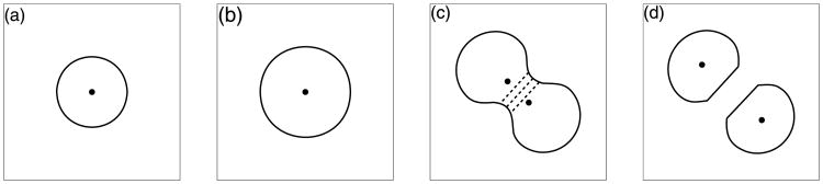
Main phases of cell proliferation: (a) cell ready to grow, (b) doubling of the cell area, (c) formation of the contractile ring (dashed lines), (d) cellular division into two daughter cells.

The orientation of cell division depends on the cell shape, its location within the cell cluster and on cell polarisation status (Section 3.7). In a dividing unpolarised cell, two new nuclei are located along the cells longest axis and the contractile ring is placed between them orthogonally to this axis in such a way as to split the cell into two approximately equal parts, Fig. 7(a). Since the location of the axis of cell division depends entirely on cell shape, unpolarised cells may have random planes of cell division. The partially polarised cell, however, acquires only one orientation of the axis of cell division that is orthogonal to the part of cell membrane that is in contact with the ECM. Two new daughter nuclei are then placed orthogonal to the axis of cell division. This gives rise to two lumenal daughter cells, Fig. 7(b).

Fig. 7.

Orientation of the axes of cell division in unpolarised (a) and polarised (b) cells, shown in dark grey with two daughter nuclei (dots), the cell longest axis (thin lines passing through daughter nuclei) and the axis of cell division (thick dashed line) that is orthogonal to the cell longest axis.

The contractile forces F_div(i) in the dividing ith cell are defined between two opposite boundary points X_i,l(t) and X_i,k(t). They act on the cell boundaries until the opposite points reach a distance ${ℒ}_{\text{div}}^{min}$, and then the dividing cell is split into two daughter cells. Each contractile force satisfies Hooke's law with the constant resting length _div and constant spring stiffness _div:

$${\mathbf{\text{F}}}_{\text{div}(i)}(l,t)={ℱ}_{\mathbf{\text{div}}}\frac{\Vert {\mathbf{\text{X}}}_{i,k}(t)-{\mathbf{\text{X}}}_{i,l}(t)\Vert -{ℒ}_{\mathbf{\text{div}}}}{\Vert {\mathbf{\text{X}}}_{i,k}(t)-{\mathbf{\text{X}}}_{i,l}(t)\Vert }({\mathbf{\text{X}}}_{i,k}(t)-{\mathbf{\text{X}}}_{i,l}(t)),$$ (9)

provided that $\Vert {\mathbf{\text{X}}}_{i,l}(t)-{\mathbf{\text{X}}}_{i,k}(t)\Vert \ge {ℒ}_{\text{div}}^{min}$ and is zero otherwise. All constants: ${ℒ}_{\text{div}}\ge {ℒ}_{\text{div}}^{\mathbf{\text{min}}}$ and _div are positive.

3.6. Cell apoptosis

An apoptotic cell undergoes very characteristic changes in its morphology, including detachment from the neighbouring cells, shrinkage of the cell volume, collapse of the cytoskeleton and alternations in the cell surface resulting in a bubbling appearance (Ardens and Wyllie, 1991). We model the process of cell apoptotic death by a gradual shrinkage of the cell area due to release of the fluid to the outside environment. This is achieved first by disassembling all cell adherens junctions and blocking them from further cell–cell contacts (Section 3.3) and by placing the sink-source couplets along the membrane of the whole cell with sinks located inside the cell and the balancing sources outside, Fig. 5(b). The resulting fluid flow causes the cell boundary to collapse and the cell area is gradually reduced until it reaches a prescribed minimal value, that we assume to be 15% of the initial cell area. At this time, the cell is considered to be dead (it is still kept in the system, but is not allowed to interact with other cells). Four stages of cell apoptotic death are manifested by a gradual reduction in cell area and changes in shape are shown in Figs. 8(a)–(d).

Fig. 8.

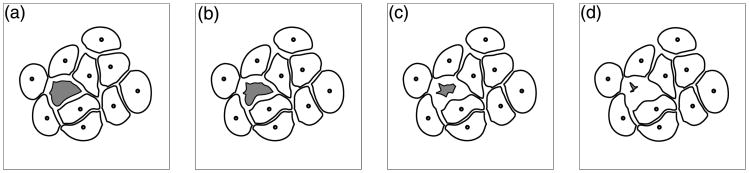
Four stages (a)–(d) of cell apoptotic death showing gradual reduction of the cell area, changes in the cell shape and shrinkage of the cell membrane.

3.7. Cell polarisation

The mature epithelial cells acquire three different cell membrane domains: an unbounded apical side facing free space inside the epithelium (lumen) and two bounded sides that are in direct contact with either the extracellular matrix (a basal side) or the membranes of other cells (lateral sides), compare Nelson (2003) and Fig. 9. During the formation of an epithelial layer in growing acini, the cells must distinguish between these different domains in order to undergo the process of cell epithelial polarisation. Since a layer of polarised cells is established before formation of the lumen (Debnath et al., 2002), cell partial polarity is determined by recognising lateral and basal sides only, whereas full polarity is acquired by developing the apical side and tight junctions along its lateral sides.

Fig. 9.

Three kinds of cell membrane domains: basal (thick grey lines) in direct contact with the extracellular matrix; lateral (thick black lines) between two neighbouring outer cells; apical (thin black lines) facing the hollow lumen.

We model cell polarisation as a multi-step process via the development of three distinct membrane domains using the following conditions (for specific details on implementation see Section 4.1):

• The cell can determine its basal side by sensing contact with the extracellular matrix (Section 3.2), all membrane receptors that express contact with the extracellular matrix constitute the basal membrane domain.

• A lateral side between two outer neighbouring cells ith and jth is formed by transforming the cell–cell connections defined between their receptors X_i,k and X_j,l into lateral connections; we introduce lateral adhesive springs F_lat(i,j) between them (Section 3.3).

• The cell is considered to be partially polarised, if it has developed an adequately long basal domain (we assume at least 25% of cell receptors), two lateral domains (each containing at least 10% of cell receptors), and if it has the potential to develop an apical side, that is, if it has contacts, with some inner cells that may be transformed into apical sites.

• The partially polarised cell becomes fully polarised when a certain percent (we assume here 75%) of its lateral connections are transformed into tight junctions (Section 3.3). Then the cell develops its free apical side by disassembling all adherens junctions expressed on the side opposite to the basal domain and disjoint from the lateral domains. Once the cell is fully polarised, it maintains a free apical side by blocking all potential adherent contacts.

Figure 9 shows different cell membrane domains in the developing acini. The basal domains (thick grey lines) occupy parts of the cell membrane that are in direct contact with the extracellular matrix. The lateral sides (thick black lines) are developed between two outer neighbouring cells in the form of short adhesive forces. The apical membrane domains (thin black lines) are located opposite to the basal domains and face the hollow lumen.

4. Mathematical framework

Our mathematical model is based on the immersed boundary method and captures interactions between elastic cells and a viscous incompressible fluid representing the cytoplasm inside the cells, the extracellular matrix outside the tissue and the lumen inside the hollow acinar structure. The fluid flow is influenced by couplets of fluid sources and sinks used to model transport of fluid across the cell membranes, as well as forces generated by the elastic cell boundaries, while at the same time the elastic structures move at the local fluid velocity. The strength of this method is that it can handle the complicated and time dependent geometry of the elastic immersed boundaries which interact with the fluid, and that it does so while using a fixed regular lattice for the fluid computation.

The model is defined on a two-dimensional domain Ω with Cartesian coordinates x = (x₁, x₂). The elastic membranes of all cells form a collection Γ of closed curves defined in the curvilinear coordinates X_i(l, t), where l is a position along the boundary of the ith cell. The fluid inside and outside the cells is modelled as a homogeneous continuum with the same constant density ρ and viscosity μ. The sources and sinks used to model the transport of fluid across the cell membrane are placed in the fluid domain along the cell boundaries. The boundary forces arise from elasticity of the cell plasma membrane (adjacent and supportive forces), division of a host cell into two daughter cells (contractile forces) and from interactions between distinct cells (lateral and repulsive forces). We assume that the fluid motion is governed by the Navier–Stokes equations:

$$\rho (\frac{\partial \mathbf{\text{u}}(\mathbf{\text{x}},t)}{\partial t}+(\mathbf{\text{u}}(\mathbf{\text{x}},t)\cdot \nabla )\mathbf{\text{u}}(\mathbf{\text{x}},t))=-\nabla p(\mathbf{\text{x}},t)+\mu \Delta \mathbf{\text{u}}(\mathbf{\text{x}},t)+\frac{\mu }{3\rho }\nabla s(\mathbf{\text{x}},t)+\mathbf{\text{f}}(\mathbf{\text{x}},t),$$ (10)

where ρ is the fluid density, p is the fluid pressure, μ is the fluid viscosity, s is the local fluid expansion, and f is the external force density. The source-sink distribution and the external forces are taken around each cell separately and then collectively applied to the fluid, that is s(x, t) = Σ_is_i(x, t) and f(x, t) = Σ_if_i(x, t).

The continuity equation with a source term describes the law of mass balance, where the source distribution s is identically equal to zero on the whole fluid domain except at the isolated point sources and sinks that are used to model the growth and death of cells:

$$\rho \nabla \cdot \mathbf{\text{u}}(\mathbf{\text{x}},t)=s(\mathbf{\text{x}},t).$$ (11)

Conservation of mass must be preserved globally in the fluid domain Ω at each time t; that is, ∫_Ωs dx = ρ ∫_Ω (∇ · u)dx = 0.

The source-sink distribution for the ith cell is composed of point sources Y_i,k and point sinks Z_i,m located around the cell boundary and then transmitted to the surrounding fluid using the two-dimensional Dirac delta function, δ(x) = δ(x₁) · δ(x₂):

$$s_i(\mathbf{\text{x}},t)=\sum _{k\in {\Xi }_i^{+}}{S}_{+}({\mathbf{\text{Y}}}_{i,k},t)\delta (\mathbf{\text{x}}-{\mathbf{\text{Y}}}_{i,k})+\sum _{m\in {\Xi }_i^{-}}{S}_{-}({\mathbf{\text{Z}}}_{i,m},t)\delta (\mathbf{\text{x}}-{\mathbf{\text{Z}}}_{i,m}).$$ (12)

The boundary forces F_i(l, t) in the ith cell X_i(l, t) represent the sum of five different forces arising from the elasticity of cell plasma membrane (adjacent F_adj(i) and supportive F_sup(i) forces), division of a host cell into two daughter cells (contractile forces F_div(i)) and from interactions between distinct cells (repulsive F_rep(i) and lateral adhesion F_lat(i) forces):

$${\mathbf{\text{F}}}_i(l,t)={\mathbf{\text{F}}}_{\text{adj}(i)}(l,t)+{\mathbf{\text{F}}}_{\text{sup}(i)}(l,t)+{\mathbf{\text{F}}}_{\text{div}(i)}(l,t)+{\mathbf{\text{F}}}_{\text{rep}(i)}(l,t)+{\mathbf{\text{F}}}_{\text{lat}(i)}(l,t).$$ (13)

They are then transmitted to the surrounding fluid using the two-dimensional Dirac delta function δ:

$${\mathbf{\text{f}}}_i(\mathbf{\text{x}},t)=\underset{\Gamma \iota }{\int }{\mathbf{\text{F}}}_i(l.t)\delta (\mathbf{\text{x}}-{\mathbf{\text{X}}}_i(l,t))\mathit{\text{dl}}.$$ (14)

The no-slip condition of a viscous fluid implies that the material points on cell boundaries are carried along with the fluid:

$$\frac{\partial {\mathbf{\text{X}}}_i(l,t)}{\partial t}=\mathbf{\text{u}}({\mathbf{\text{X}}}_i(l,t),t)=\underset{\Omega }{\int }\mathbf{\text{u}}(\mathbf{\text{x}},t)\delta (\mathbf{\text{x}}-{\mathbf{\text{X}}}_i(l,t))d\mathbf{\text{x}}$$ (15)

and the same takes place for the cell point nuclei.

4.1. Numerical implementation

In order to numerically implement the model described above, we discretise the fluid domain Ω using a uniform square grid with a constant mesh width h. Similarly, the cell membranes are represented by Lagrangian points X_l with boundary points separation of Δl ≈ h/2. The computation proceeds in time steps of duration Δt. For convenience, we use the superscript notation, that is uⁿ(x) = u(x, n Δt). At the end of time step n, the fluid velocity field uⁿ and the configuration of the boundary points ${\mathbf{\text{X}}}_l^n$ are known. These values are updated at the next time step in the following way:

1. Determine the source-sink distribution Sⁿ at points Y_k and Z_m located along the boundaries of all expanding or shrinking cells (growing, dying or resting cells which areas exceed homeostatic limits); spread these values to the neighbouring grid points to find the local expansion rate sⁿ of the fluid:

   $$s^n(\mathbf{\text{x}})=\sum _i(\sum _{k\in {\Xi }_i^{+}}{S}_{+}^n({\mathbf{\text{Y}}}_{i,k},t){\delta }_h(\mathbf{\text{x}}-{\mathbf{\text{Y}}}_{i,k})+\sum _{m\in {\Xi }_i^{-}}{S}_{-}^n({\mathbf{\text{Z}}}_{i,m},t){\delta }_h(\mathbf{\text{x}}-{\mathbf{\text{Z}}}_{i,m})).$$ (16)

2. Calculate the total force density Fⁿ from the configuration of cell boundaries; spread those values to the neighbouring grid points to determine the forces fⁿ acting on the fluid:

   $${\mathbf{\text{f}}}^n(\mathbf{\text{x}})=\sum _i(\sum _i{\mathbf{\text{F}}}_i^n(l,t){\delta }_h(\mathbf{\text{x}}-{\mathbf{\text{X}}}_{i,l})\Delta l),$$ (17)

   where

   $${\mathbf{\text{F}}}_i^n(l,t)={\mathbf{\text{F}}}_{\text{adj}(i)}^n(l,t)+{\mathbf{\text{F}}}_{sup(i)}^n(l,t)+{\mathbf{\text{F}}}_{\text{div}(i)}^n(l,t)+{\mathbf{\text{F}}}_{\text{rep}(i)}^n(l,t)+{\mathbf{\text{F}}}_{\text{lat}(i)}^n(l,t).$$

3. Solve the Navier–Stokes equations for the fluid velocity field uⁿ⁺¹ by using the fast Fourier transform algorithm with periodic boundary conditions imposed on the fluid domain. The equations are discretised using the first order finite difference scheme with the spatial difference operators: forward D⁺, backward D⁻, centred D⁰ and upwind D^±; r = 1, 2 denotes the first and second vector field components, respectively:

   $$\{\begin{array}{l}\rho (\frac{u_r^{n+1}-u_r^n}{\Delta t}+{\sum }_{s=1}^2{u}_s^n{D}_s^{\pm }{u}_r^n)=-D_r^0{p}^{n+1}+\mu {\sum }_{s=1}^2{D}_s^{+}{D}_s^{-}{u}_r^{n+1}+\frac{1}{3}\frac{\mu }{\rho }{D}_r^0{s}^n+f_r^n,\hfill \\ \rho {\sum }_{s=1}^2{D}_s^0{u}_s^{n+1}=s^n.\hfill \end{array}$$ (18)

4. Interpolate the fluid velocity field uⁿ⁺¹ to each immersed boundary point and compute their new positions ${\mathbf{\text{X}}}_l^{n+1}$ by moving them at the local fluid velocity using a forward Euler step:

   $$\begin{array}{c}{\mathbf{\text{u}}}^{n+1}({\mathbf{\text{X}}}_l^n)=\sum _{i,j}{\mathbf{\text{u}}}^{n+1}({\mathbf{\text{x}}}_{i,j}){\delta }_h({\mathbf{\text{x}}}_{i,j}-{\mathbf{\text{X}}}_l^n)h^2,\\ {\mathbf{\text{X}}}_l^{n+1}={\mathbf{\text{X}}}_l^n+\Delta t\cdot {\mathbf{\text{u}}}^{n+1}\left({\mathbf{\text{X}}}_l^n\right).\end{array}$$ (19)

Interactions between the fluid grid and the material points are implemented using the discrete approximation δ_h(x) to the Dirac delta function, where δ_h(x) = δ_h(x₁) δ_h(x₂), and

$${\delta }_h(\mathbf{\text{r}})=\{\begin{array}{ll}\frac{1}{4h}(1+cos(\frac{\pi r}{2h}\left)\right)\hfill & \text{if}\left|r\right|<2h,\hfill \\ 0\hfill & \text{if}\left|r\right|\ge 2h.\hfill \end{array}$$ (20)

More details about the numerical implementation of this algorithm and the numerical solution of the Navier–Stokes equations can be found in Rejniak (2002), Rejniak et al. (2004).

In principle, it is enough to store only the positions of all boundary points for each cell to be able to re-compute the cell phenotypic state, and all cell–cell and cell–ECM connections. For example, after discretisation, the microenvironment of each cell receptor contains only finitely many points that can be directly inspected. However, to simplify computations and to reduce usage of searching algorithms, we remember type of each cell receptor by using the following markers: zero denotes a free receptor; a positive number identifies an index of the co-adherent point located on the boundary of the neighbouring cell; −1 represents contact with the extracellular matrix; −0.5 denotes the blocked receptor. Since we start each simulation with a single cell, all of its receptors initially are in contact with the ECM. They can be transformed into cell–cell adhesive connections as a result of cell division and the emergence of daughter cells. The cell–cell adhesive connections are updated after each cell division and new connections are determined by inspecting receptors of neighbouring cells whose nuclei are located within two cell diameters of the host cell. The cell–cell adhesive connections between outer cells are considered tight junctions if they are sufficiently close. Free receptors are created during cell growth as a result of expansion of the cell membrane where new points are introduced between already existing receptors. Blocked receptors emerge as a result of removal of adherent connections on an apical membrane domain and along the boundary of each apoptotic cell.

4.2. Scaling of the equations

In order to cast the governing equations into dimensionless form, we introduce the characteristic length L and velocity U scales. The scaled variables are then defined as follows: τ = t/T, x̂ = x/L, X̂ = X/L, û= u/U, p̂ = p/P, ŝ= s/S, where we set T = L/U. The dimensionless equations have then the following form:

$$\begin{array}{l}\frac{\partial \stackrel{\wedge }{\mathbf{\text{u}}}}{\partial \tau }+(\stackrel{\wedge }{\mathbf{\text{u}}}\cdot \nabla )\stackrel{\wedge }{\mathbf{\text{u}}}=-\nabla \stackrel{\wedge }{p}+\frac{1}{\mathit{\text{Re}}}(\Delta \stackrel{\wedge }{\mathbf{\text{u}}}+\frac{1}{3}\nabla \stackrel{\wedge }{s})+\stackrel{\wedge }{\mathbf{\text{f}},}\hfill \\ \nabla \cdot \stackrel{\wedge }{\mathbf{\text{u}}}=\stackrel{\wedge }{s},\hfill \\ \stackrel{\wedge }{\mathbf{\text{f}}}(\stackrel{\wedge }{\mathbf{\text{x}}},\tau )=\int \stackrel{\wedge }{\mathbf{\text{F}}}(\sigma ,\tau )\delta (\stackrel{\wedge }{\mathbf{\text{x}}}-\stackrel{\wedge }{\mathbf{\text{X}}}(\sigma ,\tau ))d\sigma ,\hfill \\ \stackrel{\wedge }{s}(\stackrel{\wedge }{\mathbf{\text{x}}},\tau )=\sum {\stackrel{\wedge }{S}}_{+}(\stackrel{\wedge }{\mathbf{\text{Y}}},\tau )\delta (\stackrel{\wedge }{\mathbf{\text{x}}}-\stackrel{\wedge }{\mathbf{\text{Y}}})+\sum {\stackrel{\wedge }{S}}_{-}(\stackrel{\wedge }{\mathbf{\text{Z}}},\tau )\delta (\stackrel{\wedge }{\mathbf{\text{x}}}-\stackrel{\wedge }{\mathbf{\text{Z}}}),\hfill \\ \frac{\partial \stackrel{\wedge }{\mathbf{\text{X}}}(\sigma ,\tau )}{\partial \tau }=\stackrel{\wedge }{\mathbf{\text{u}}}(\stackrel{\wedge }{\mathbf{\text{X}}}(\sigma ,\tau ),\tau ),\hfill \end{array}$$ (21)

where Re = ρLU/μ is the Reynolds number and the remaining quantities are defined as p̂ = p/(ρU²), f̂ =fL/(ρU²), ŝ = sL/(ρU) and σ = l/L. For a characteristic length-scale, we take the diameter of a well-developed acinus L = 65 μm (from figures in Debnath et al. (2002)). The characteristic velocity-scale reflects an increase in the diameter of the acinar cluster from 35 μm to 65μm over a period of 3 days, as reported in Debnath et al. (2002) for in vitro experiments on the MCF-10A cells. This gives a characteristic time scale of T = 6.5 days, and one step of the computational algorithm corresponds to about 2 minutes of real time. Following Dembo and Harlow (1986) and Laurent et al. (2003), we take values of fluid density ρ = 1.35 g/cm³ and fluid viscosity μ = 100 g/(cms), that both correspond to the rheological properties of the network part of the cytoplasm. This gives a near-zero Reynolds number indicating that the viscous effects dominate the inertial ones in the cytoplasmic flow during the acinar development. The values of other parameters are chosen to fit known qualitative behaviour of the growing acini. The rigidity of the elastic cortical cytoskeletal network associated with the plasma membrane in the adherent epithelial cells is in the range of 490–850 g/(cms²) (Laurent et al., 2003), and we take _adj = _sup = 500 g/(cms²) as a stiffness constant of all adjacent and supporting force densities. Similarly, stiffness constants _rep of the repulsive and _lat of the lateral contractile force densities are taken equal to _adj to equalise their impact on the common boundary point. The value of the contractile spring stiffness and the strength of fluid sources and sinks for each channel have been determined computationally to match the dynamics of proliferating and dying cells, respectively. A good match for the average time needed for growth and division of several cells in a small cluster and for apoptotic death of a single cell, as well as for acquiring cell shapes during these processes has been achieved for source and sink strengths of ${\mathcal{\text{S}}}_{+}^0={\mathcal{\text{S}}}_{=}^0=5\times {10}^{-10}\text{g}/\text{s}$, and a contractile spring stiffness of _div = 50 × _adj. All other computational parameters are defined in terms of the mesh width h and a boundary point separation Δl as follows: the resting length of all adjacent springs is equal to the initial cell separation _adj = Δl, whereas the resting length of all supportive springs is twice as long, i.e. _sup = 2Δl. The resting length of all repulsive forces is equal to the mesh width _rep = h, and the resting length of all lateral springs is equal to half of the mesh width, i.e. _lat = 0.5h. The resting length of all contractile springs is L_div = 5Δl. The radius of a local microenvironment for assembling cell–cell connections is equal to ${ℒ}_{\text{adh}}^{max}=2h$, whereas the radius of a local microenvironment for fluid transport equals a mesh width ε_tr = h.

5. Computational results

We first present a detailed simulation of our model showing several stages of acinar development, starting from a single cell which gives rise to a cluster of randomly oriented cells, that subsequently either transform into polarised cells or die leading to the formation of a stable hollow structure, Section 5.1. In Section 5.2, we analyse the dynamics of acinar development by discussing cellular processes occurring in two distinct regions occupied either by inner or outer cells and their role in the formation of the epithelial layer and the hollow lumen. A more detailed look at changes in the proportions of phenotypically different cells that arise during the acinar development is presented in Section 5.3 together with the evidence for biologically realistic timing of the processes of cell growth, division and apoptosis. In Section 5.4, we present results of several simulations of distinct epithelial acini and discuss relations between cell maturation, duration of cell proliferation and the time of initiation of cell polarisation that can lead to the formation of epithelial acini of different sizes and of regular or degenerate shapes.

5.1. Development of a typical hollow acinus

Dynamical development of a typical hollow acinus is presented in a series of snapshots in Fig. 10 that allow for simultaneous comparison of two different types of data at the same time points. Figures 10(a1)–(j1) show colour-coded subpopulations of cells of different phenotypes: growing cells are shown in green, outer resting cells are yellow, inner resting cells are blue, partially polarised cells are pink, fully polarised cells are red, apoptotic cells are grey, and dead cells are represented by black points. Figures 10(a2)–(j2) show intracellular elements for each individual cell and intercellular elements between separate cells and between cells and the extracellular matrix. The nuclei of living cells are stained in blue, the nuclei of apoptotic cells are red, cell membranes are shown in green, lateral membrane domains between neighbouring cells are stained in white, tight cell–cell junctions are yellow, and the basal membrane domains are shown in pink. This side-by-side comparison of two different sets of snapshots from the very same simulation allows one to observe how interactions between separate cells and between the cells and their microenvironment determine the cell phenotype. The presented simulation follows a typical pathway of acinar development—starting from a single cell, Fig. 10(a), that upon consecutive divisions gives rise to a small cluster of randomly oriented cells, Fig. 10(b). Further proliferations lead to the formation of a larger group of cells that self-organise into a two-population cluster containing outer and inner cells, Figs. 10(c)–(d). The outer cells acquire an apical-basal polarisation due to the interactions with their neighbours, Figs. 10(e)–(f), that is followed by their differentiation leading to the formation of one layer of polarised cells, Figs. 10(g)–(j). This in turn triggers the inner cells to die by apoptosis, Figs. 10(f)–(i), which results in the formation of the hollow lumen, Figs. 10(i)–(j). Due to suppression of the growth of fully polarised cells the final structure stabilises in the form of a hollow acinus, Fig. 10(j), in which the inner lumen is surrounded by a single layer of eukaryotic cells forming an epithelium.

Fig. 10.

Development of a typical epithelial acinus. Left and right columns show different subpopulations of epithelial cells: green—growing, yellow—resting outer, blue—resting inner, pink—partially polarised, red—fully polarised, grey—apoptotic, black points—dead. Two middle columns show inter- and intra-cellular elements: blue—nuclei of living cells, red—nuclei of apoptotic cells, green—cell membranes, white—lateral membrane domains, yellow—tight junctions, pink—basal membrane domains. A hollow epithelial acinus develops from a single cell (a) that upon consecutive divisions gives rise to a small cluster of cells (b), further growth leads to the formation of phenotypes of outer and inner cells (c)–(d), due to interactions with neighbouring cells the phenotypes of partially and fully polarised cells emerge (e), first apoptotic cells arise in the neighbourhood of fully polarised cells (f), centrally located inner cells die due to lost of adhesive support from neighbouring cells (g)–(h), the growth of fully polarised cells is suppressed that leads to structure stabilisation (i)–(j). The time points shown correspond to real time: (a) 9.25 hours, 13 μm in diameter; (b) 3.85 days, 21 μm; (c) 8 days, 38 μm; (d) 10.75 days, 50 μm; (e) 13.85 days, 64 μm; (f) 15 days, 69 μm; (g) 15.75 days, 71 μm; (h) 16.5 days, 72 μm; (i) 17.5 days, 72 μm; (j) 19.25 days, 72 μm in diameter. A supplementary movie is available online: http://www.maths.dundee.ac.uk/∼rejniak/BMBmovie.html.

The ten different snapshots presented in Fig. 10 show specific stages of acinar development that represent important time points at which certain subpopulations of phenotypically different cells change their dynamics—for instance, a new cell phenotype can emerge, or it can disappear, or some cell phenotypes start dominating the whole cell cluster. In Fig. 10(a), one single round cell is shown at time corresponding to 9.25 hours of its real growth. Initially, the cell had a diameter of 10 μm and during the time considered here, it gained an additional 3 μm. Note, that this cell remains circular due to the uniform distribution of fluid channels around the cell boundary. Figure 10(b) shows a cluster of four resting cells after 3.85 days of real time. All four cells have contact with the extracellular matrix, so all of them are classified as outer cells. Each pair of neighbouring cells has already developed cell–cell connections and some of them are close enough to form tight junctions (white and yellow staining of common cell boundaries in Fig. 10(b2)). The slight asymmetry of the whole cluster is an effect of uneven cell growth and division. Small differences in the location of fluid sources and sinks along the boundary of growing cells results in an asymmetric fluid flow, and then in an asymmetrically shaped daughter cells that can have different numbers of boundary points—here, cells contain from 64 to 68 points. This is further amplified leading to irregularly shaped acini that, however, resemble real experimental data. Figure 10(c) shows a small asymmetric, cluster of an average diameter of 38 μm after 8 days of development. A newly emerged subpopulation of three inner cells (green here, since they are growing) is surrounded by ten outer resting cells (yellow). This cluster expands further over the next 2.75 days reaching 21 cells and an average diameter of 50 μm, Fig. 10(d). At this stage, the cluster contains resting inner cells (blue), resting outer cells (yellow) and a few growing cells (green) at different locations within the cluster. Figure 10(e) shows two new cell phenotypes—partially polarised cells (pink) and fully polarised cells (red).

To become partially polarised, the outer cells must develop two lateral sides with other outer cells, an adequately long basal side facing the extracellular matrix and have the potential to develop an apical side, for instance, by expressing the adhesive connections with inner cells. Note, that two other non-growing outer cells (yellow) are not transformed into the partially polarised phenotype, since they either are not in contact with enough of the external medium (the left yellow cell), or have no potential to develop an apical side—being in contact only with two other outer cells (the right yellow cell). The cell transformation into a fully polarised phenotype requires a development of tight junctions on each lateral membrane domain and creation of a free apical side by breaking all cell– cell connections along its apical membrane domain. All other outer cells in Fig. 10(e) are actively proliferating and even if they satisfy polarity conditions, they must first complete any initiated process of growth and division. Note, that many of them become polarised (compare Fig. 10(f)) and remain fully polarised in all subsequent snapshots. Nine inner resting cells (blue) have insufficient free space to grow, since they are too crowded by other cells. The whole cluster is 64 μm in diameter and corresponds to 13.85 days of real time. Figure 10(f) shows the initial formation of a layer of partially and fully polarised cells around the perimeter of the whole cluster. The two first apoptotic cells (grey) arise due to the loss of adhesive connections. This happens in the neighbourhood of one fully polarised cell as a result of the development of its free apical membrane domain. Again, numerous inner cells are resting due to insufficient space for growth. All others are actively proliferating. Note two dividing cells that possess two daughter nuclei, Fig. 10(f2). Both of them are located on the cluster boundary, but due to their different shapes after doubling their areas, one of the cells divides parallel and the other perpendicular to the extracellular matrix. The cell in the upper-left part of the cell cluster will give rise to one inner and one outer daughter cell, whereas the cell located in the lower-right part of the cell cluster will give rise to two outer daughter cells. The whole cluster reaches 69 μm in diameter and it corresponds to the formation of an epithelial cluster after 15 days of real time. Figure 10(g) shows further development of an outer layer of fully polarised epithelial cells. Note, that two of the partially polarised cells from a previous snapshot have started a process of cell growth, but all others turned into fully polarised cells. Two apoptotic cells from the previous snapshot died (black dots), similarly for four previously inner resting cells in the upper part of the lumen. Seven other inner cells started the process of cell apoptotic death due to loss of adhesive support either from the fully polarised cells in their neighbourhood or from other dying cells. This leads to the expansion of the hollow lumen. Note that since some of the inner cells are still growing, multiple lumens are created inside the acinar cluster. The average diameter of the presented structure is 71 μm and corresponds to acinar development at 15.75 days of real time. Figure 10(h) shows an acinus after 16.5 days of development. Its average diameter of 72 μm is almost unchanged compared to the previous snapshot. There are still a few proliferating cells inside the cell cluster and on its boundary, but most of inner cells are apoptotic and most of outer cells are already fully polarised. The further lumen expansion and increase in the number of fully polarised cells is shown in Fig. 10(i), corresponding to 17.5 days of acinar development. The full stabilisation of the acinar structure is achieved at 19.25 days and is shown in Fig. 10(j). The whole cluster reaches 72 μm in diameter, the outer epithelial layer contains 24 fully polarised cells. Note the well developed tight junctions between neighbouring polarised cells (yellow staining of common cell boundaries in Fig. 10(j2)).

The presented simulation shows the formation of a generic hollow acinus that follows all the developmental stages observed in biological experiments (O'Brien et al., 2002; Debnath and Brugge, 2005; Debnath et al., 2003). The snapshots presented in Fig. 10 are in good qualitative agreement with pictures of real acini shown in Fig. 1. In particular, Fig. 1(a) and Fig.10(c), both show small clusters of randomly oriented cells at time corresponding to day 8 of real time. Figure 1(b) shows two real acini after 16 days of growth. The formation of one layer of outer cells and the emergence of hollow lumen is more pronounced in the upper acinus. Figures 10(g)–(h) show simulated acini at time points 15.75 days and 16.5 days. In both cases, the outer epithelial layer is partially formed and the free space inside the structure is still partially filled by inner cells. The fully formed hollow structure is shown in Fig. 1(c) and Fig. 10(j) for a real acinus at day 20th, and for a simulated acinus at time corresponding to 19.25 days, respectively.

5.2. Dynamics of acinar development

Comparing several acinar configurations shown in Fig. 10, it is clear that some complex processes must occur in order to dynamically develop two acinar regions occupied by cells with very distinct fates. The cells in the outer region, having access to the extracellular matrix, remain alive and must organise themselves into one layer of tightly packed epithelial cells. The cells in the inner region contribute to the formation of the lumen by committing apoptotic death without causing any damage to the surrounding epithelium. The areas of the regions occupied by the whole acinar cluster, by the living cells and by the emerging lumen are shown in Fig. 11(a). For comparison, the evolution of the total number of cells, the count of outer cells, the number of living inner and a cumulation of dead inner cells are shown in Fig. 11(b). The simultaneous investigation of both graphs allows us to analyse the dynamics of acinar development, the progress in formation of the hollow lumen and the stability of the complete structure. Figures 11(c)–(d) show the proportions of growing and non-growing cells in each region, the non-growing cells include either the outer polarised cell or the inner resting cells.

Fig. 11.

(a) Dynamical changes in the total area of the cluster (1), the area of a subregion occupied by the living cells (2), and a subregion occupied by the lumen (3); (b) evolution of the total number of cells in the whole cluster (1), the accumulation of dead cells (2), the number of inner living cells (3), the number of outer cells (4); (c) evolution of the number of outer cells: (4) total, (4p) polarised, (4g) growing cells; (d) evolution of the number of inner cells: (3) total, (3r) resting, (3g) growing cells; horizontal lines below the graph indicate time intervals in which particular cell subpopulations are present in the system.

The area of the whole acinus is calculated as the space enclosed by the basal membrane, a curve composed from basal membrane domains of all outer cells (the pink curve in Figs. 10(a2)–(j2)). The area occupied by all living cells is calculated as the sum of areas of those cells that are not dead, including the diminished apoptotic cells. The area that is not occupied by the cells but it is enclosed by the basal membrane is considered to be filled with the lumen. Note that the lumen is present inside the acinar structure from a very early stage of its development (line (3) in Fig. 11(a)), but initially it is created as a result of small lumenal spaces between newly born daughter cells (compare Figs. 10(b1)– (c1)). The total amount of the lumen is, however, insignificant until the 5th day when the first inner cells emerge and then it increases slowly but steadily until the 15th day when the first apoptotic cells arise. After this time, the amount of the lumen inside the acinar cluster grows rapidly in accordance with the increased cell death, compare line (3) in Fig. 11(a) and line (2) in Fig. 11(b) after day 15. Finally, the area filled by the lumen overtakes the area occupied by outer polarised cells by about 10% and both values saturate after day 17, compare lines (2) and (3) in Fig. 11(a). Moreover, the number of outer cells becomes unchanged over the same period of time, that confirms final stabilisation of the whole acinar structure. Before the initiation of apoptotic events at day 15, almost all space inside the acinus was occupied by the living cells that is verified by almost overlapping area curves (1) and (2) in Fig. 11(a). The wavy appearance of both of them is a result of alternating periods of cell proliferation (oblique segments) and cell maturation before entering in the new growing period (plateaus), compare yellow resting cells and green growing cells in Figs. 10(b1)–(e1). After day 15, the area occupied by living cells decreases rapidly due to the increased rate of cell death and decreased rate of cell birth. Finally, it stabilises around day 17, as does the number of cells in the outer layer; compare curves (2) in Fig. 11(a) and (1) in Fig. 11(b).

Changes in cell counts from growing acini are shown in Fig. 11(b) for three different groups: outer, living inner and dead cells, and additionally for the total number of cells in the cluster. Figures 11(c)–(d) show the further partition into growing and resting subpopulations of the inner and outer cells, respectively. Each horizontal line below the graphs corresponds to a particular subpopulation of cells and indicates the time interval at which this subpopulation is present in the whole acinar cluster. Initially, the acinar cluster contains only outer cells, since all of them are in contact with the extracellular matrix. The general tendency in the increase of the number of outer cells during the whole time of acinar development has a linear characteristics since these cells are located in a single layer along the cluster perimeter and, except for a short time needed for cell maturations just after they are born, they grow instantly due to the available space in the surrounding extracellular matrix, compare lines (4) and (4g) in Fig. 11(c). The long plateaus indicate periods of time when the outer cells are either maturating or actively growing, so the overall number of cells is unchanged. Note, that for the maturation periods, the curve (1) in Fig. 11(a) showing the total area of the cell cluster has also small plateaus, whereas for the proliferation periods, it shows increase in the total area. At the later stages of the acinar development, the plateaus of outer cells include the partially and fully polarised cells and the saturation after the 17th day which includes only fully polarised cells. At a few points a sharp decrease in the number of outer cells is visible. This is due to the passive dislocation of those outer cells towards the middle of the cell cluster followed by the loss of their connections with the extracellular medium that results in the change of their phenotypes into inner cells. Note that the number of the inner cells increases at these very points. The reason for such dislocation of some outer cells is their weak contact with the extracellular matrix that is easily lost due to the tension from their growing neighbours. However, such dislocation is in general a quite rare event and the majority of inner cells arise due to cell unpolar division. First inner cells emerge shortly after the 5th day, and the initial phase of its development is characterised by long periods of constant cell counts due to the fact that growing cells need time to double their areas and to divide, compare curves (3) and (3g) in Fig. 11(d). Then the total number of cells increases exponentially since the majority of cells are actively growing (compare also Fig. 10(e1)). These dynamics change when the apoptotic cells emerge, as this results in a rapid decrease in the number of inner cells since most of them die by apoptosis, curve (3r) in Fig. 11(d). However, cell growth is still present in the subpopulation of inner cells, curve (3g) in Fig. 11(d). Finally, the number of inner cells falls to zero, and the saturation of the number of total cells coincides with the number of outer cells.

5.3. Evolution of emerging cell subpopulations

Development of the whole hollow acinus from a single eukaryotic cell requires first an extensive cell proliferation to build a solid spherical structure, then transformation of all outer cells into an epithelial layer, and finally a massive death of inner cells to form the lumen. In this section, we consider subpopulations of cells that differ in their activities independent of their location within the cluster. The dead cells will be disregarded since they do not contribute to any changes in the acinar structure. Therefore, we focus our attention on four cell subpopulations—the growing, apoptotic, partially and fully polarised cells. We look more closely at changes in the proportions of these phenotypically different cell subpopulations during the acinar development. We also discuss evidence that the timing of cell growth, division and apoptosis is modelled within biologically realistic limits.

Figure 12 shows the time evolution of cell counts for four different cell subpopulations: the growing, apoptotic, partially and fully polarised cells. In each horizontal line below, the graphs correspond to a particular subpopulation of cells and indicates the time interval at which this subpopulation is present in the whole acinar cluster. The underlying assumption of our model is that each undifferentiated cell (inner or outer) maintains its cell cycle by continuously checking if there is enough free space around it to acquire the fluid necessary for its growth. The transport of fluid only takes place along the part of the cell membrane that is not in contact with other cells. Therefore, the time needed to double the cell area depends on cell shape and location, and on the number of water channels that are available. If the growing cell becomes too crowded by other cells and its membrane receptors become blocked by adhesive contacts with other cells, the host cell stops growing. All these assumptions imply that the growth curve (line (2) in Fig. 12) spans the time interval from the beginning of the acinar development to the time of acinar stabilisation, when all outer cells acquire the polarised phenotype, and all inner cells become extinct. Since cell growth in our model is time dependent, the growing curve contains multiple periods alternating between long plateaus (when the cells are growing, so their number is constant) and short steeply increasing segments (when the new daughter cells enter into the growing period after their maturation). The sharp short decreases in the number of growing cells in the first half of the acinar development indicate these times at which the inner cells are too crowded to be able to start or continue the growth process, so their phenotype changes from growing to resting. The steady decrease in the number of growing cells arising around the 14th day coincides with the emergence of fully polarised cells that are growth-suppressed, this decrease persists due to the increased apoptotic death of inner cells, Figs. 10(f)–(g). However, the incidentally proliferating cells are present to the very end of the acinar development, Fig. 10(i). The apoptotic cells are present in our system only for a short period of time between days 15 and 18, and at their peak, there are as much as 10 cells simultaneously dying. The partially polarised cells arise first around day 11 and reach their first peak value of 7 cells at day 13. Most of them, however, enter again into the growing phase without differentiation into the fully polarised phenotype. The second peak value of 5 partially polarised cells is reached at day 15, but this time the majority of cells undergo a transformation into the fully polarised phenotype. The number of fully polarised cells is very small between the 12th and 14th days, but then increases steadily up to the 19th, when the entire outer layer is composed of fully polarised cells forming the epithelium.

Fig. 12.

Evolution of four subpopulations of phenotypically distinct cells leading to the formation a hollow epithelial acinus: (1) apoptotic cells, (2) proliferating cells, (3) partially polarised cells, (4) fully polarised cells; horizontal lines below the graph indicate time intervals in which particular cell subpopulations are present in the whole system.

Since model parameters were chosen to match the dynamics of cell processes in a small cluster of individual cells, but then were applied to larger populations of interacting cells, all growing and dying cells in our system were traced to determine distributions of the time needed for completion of three life cycle processes: cell growth, division and apoptosis. Figures 13(a)–(c) show the data obtained for 54 proliferating and 31 dying cells. The mean time needed for doubling of the area of a growing cell shown in Fig. 13(a) is about 39.8 hours, but the actual time for different cells varies from 10 to 70 hours and strongly depends on the location of the growing cell within the acinar cluster. We assume that each water channel used to transport the water from the extracellular matrix to the cell interior has a constant flow rate, and therefore, the speed of cell growth depends on the number of available water channels (Section 3.4). The first growing cell doubles its area in only 10 hours, since it is surrounded entirely by the extracellular matrix and can acquire water through its whole membrane. Its two daughter cells need about 30 hours each for doubling their areas, since some boundary receptors are in contact with the other cell and thus are blocked from transporting the water from the extracellular space. A few cells located inside the cell cluster require more than 60 hours to double their areas. They were able to sense enough free space around them to initiate the process of cell proliferation, but their growth is significantly slower due to cell overcrowding. Figure 13(b) shows the distribution of times needed to complete the division of the mother cell into two daughter cells. The average time of cell division is about 8.2 hours, but the actual time varies for different cells and strongly depends on the cell shape and on its location within the acinar cluster. The contractile ring splitting the cell into two daughters is defined as a collection of contractile forces of a constant strength, thus the time needed for bringing two opposite sides of the cell boundary together depends on the distance between them (Section 3.5). Since cells from a few initial generations are quite roundish in shape, they require more then 10 hours each to complete the process of their division. A very short time of cell mitosis was observed in those cells that were already narrow and elongated, so the distance between opposite sides of their contractile rings was small. Figure 13(c) shows a distribution of the time needed for completion of cell apoptosis, which is assumed, in our model, to take place when the cell area shrinks to 15% of its initial value (Section 3.6). The average time of cell apoptotic death takes 9.3 hours and does not appear to vary too much among all dying cells. This is due to the fact that apoptotic cells release the water to the extracellular space through water channels located along the whole cell membrane. Slight differences in the time of cell apoptotic death result from differences in cell shape, and thus slightly variable numbers of active water channels on the cell membranes.

Fig. 13.

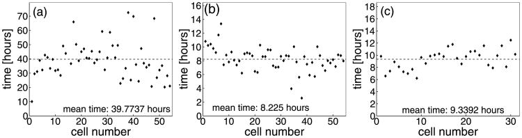
Distributions of times needed for completion of processes of cell growth (a), cell division (b), cell apoptosis (c) for 54 proliferating and 31 dying cells from the simulation in Fig. 10.

The times of cell growth, division and apoptosis observed in our simulation are biologically realistic. However, a direct comparison with the experimental data is impossible due to limited ability to trace single growing or dying cells in the acinar and other biological systems and to observe dynamical changes in cell morphology over long enough periods of time. The available experimental data on apoptotic cells (Bowen and Lockshin, 1981; Ardens and Wyllie, 1991) reveal that the first stage of cell apoptotic death resulting in a sudden cell shrinkage lasts only a few minutes, but the apoptotic cells remain recognisable within a tissue over a period of next 4–9 hours. A series of light micrographs published in Alberts et al. (2002) shows that division of a living cell from the lung epithelium of a newt takes about 6 hours. The time of cell growth and of the entire cell cycle are usually reported in the form of a cell doubling time that is determined by planting a large number of cells on flat wells and then counting them at equal time intervals to find the time point where the initial number of cell has doubled. It is believed that the cycle of normal mammalian cells lasts from 12 to 24 hours. It is also known, however, that most of cells in the living body are in the quiescent non-growing phase. Our simulation deals with cells that from the beginning are imposed to interactions with other cells and to signals that lead to their self-reorganisation, first into a compact cluster, then into an epithelial layer. Therefore, their behaviour may more closely resemble living cells within a tissue than individual cells planted on the laboratory well. Thus, the times needed for such cells to double their areas may be significantly different than that reported from experimental studies where all cells have enough space to grow before they are counted. Nevertheless, the average times of cell growth, division and apoptosis predicted by our model are biologically reasonable. However, it should be noted that by varying some model parameters these times can also be adjusted if more detailed experimental data were to become available.

5.4. The importance of epithelial polarisation

The epithelial acini stabilise in the form of hollow structures surrounded by a continuous layer of polarised epithelial cells. The epithelial polarisation of all outer cells in the fully developed biological acini has been confirmed through a selective staining of some intracellular components. Several specific antibodies that recognise certain proteins characteristic for tight junctions, Golgi apparatus, apical or basal-lateral domains of the cell plasma membrane have been reported in Debnath et al. (2002, 2003), Wang et al. (1990a, 1990b) to confirm polarity of epithelial cells in MDCK cysts and MCF-10A mammary acini in vitro. However, no experimental data are available that show the dynamical development of such cell polarity. Little is also known about the temporal and spatial regulations of the formation of distinct membrane domains during the morphogenesis of a polarised epithelium in vivo. In particular, no specific time regimes are known, for neither the time of initiation of the polarised transformation nor for its duration.

Using our model of acini development, we can address the question of how initiation of cell polarity affects the overall development of the acinar structure. We take into account two parameters: the time of initiation of partial cell polarisation and the duration of cell resting phase, and discuss a range of values of these two parameters that lead to the development of normal functional acini or to structures degenerate in their shape and size. The time needed for a cell to maturate right after its birth, that we also call the cell resting period represents a cell state during which no growth is allowed. Since we consider in this paper a general acinar model not adjusted to any particular cell line, this parameter is defined as a percentage of the average time of cell growth. Shortening this period of cell maturation results in an elevated frequency of cell proliferation, a higher mitotic index, a shorter doubling time, and thus a more malignant cell phenotype. Note, that the more frequent proliferation can also be a result of some selective pressure from the cell environment or some cell genetic mutations (see Anderson, 2005; Anderson et al., 2006).

The process of cell partial polarisation is not assumed to occur automatically, but we introduce a time delay that relates the initiation of the partial polarisation process with the size of the whole growing cluster. Then, the process of cell full polarisation is completed as soon as the cell develops its basal and lateral membrane domains. Such a global time delay in starting the partial polar transformation in biological acini may result from the secretion of a certain amount of the basal lamina on the contact side of the outer cells and the external medium around the whole acinar cluster. For instance, a sufficiently high concentration of the basal membrane is needed to properly define the cell apical-basal axis. Inclusion of such a time delay allows us to investigate the relationship between the frequency of initiation of cell growth in the whole cluster with the time of growth suppression due to polarisation of outer cells. We will show that by varying this two parameters our model can produce either small afunctional acini, or degenerate mutants, or normal acini of various sizes but regular shapes. Figure 14 shows four distinct regions in the considered parameter space together with representative shapes of acinar structures and the average time at which such structures become stable.

Fig. 14.

Four regions of distinct acinar development. Prolonged cell maturation together with early cell polarisation leads to small afunctional acini; fast proliferation with early cell polarisation results in degenerate mutants; coordination between cell maturation and initiation of polarisation leads to normal acini; if cell polarisation is initiated late, the acinar structures grow larger but look normal. The time needed to acquire a stable acinar structure varies: small acini stop growing very fast (14 days on average), normal and large acini need similar times (about 19 days on average), but for degenerate acini it takes longer to stabilise (23 days on average).

The results show that normal acini are formed when there is a coordination between the speed of cell growth and the time at which cell polarisation is started. All combinations of the indicated parameters were used to generate final stable acinar structures that were subsequently classified into four different groups in Fig. 14. Note that all representative acini are composed of one layer of epithelial cells enclosing the hollow lumen, however their sizes and shapes are very distinct, as is the time at which such acinar structures become stable. Generally, the longer the time of cell maturation and the later the switch in the initiation of epithelial polarisation leads to the formation of more regularly shaped acini, since the whole acinar cluster has time to gain sufficient cell mass and the individual cells have time to establish distinct membrane domains and to assemble tight cell–cell junctions. However, if such slowly maturated cells are allowed to polarise very early, when the cell cluster contains about 10 cells, the whole acinar structure stabilises quickly (14 ± 4 days). Since these cells are not forced to grow due to the long period of their maturation, they have time to adapt their shapes and to build up the proper cell–cell connections, that together with early cell polarisation results in the growth arrest of very small clusters (the average acinar cluster in this category has an area of 1829 μm² with the lumen accounting for only 37%), compare progression in cell polarisation (dark grey cells) in Figs. 15(a1)–(a3). In contrast, if cell maturation period is very short, but they polarise very early, the acinar structure acquires a degenerate form. This is because some cells were able to develop all membrane domains and cell–cell connections required for full polarisation early on, and thus their further growth is suppressed (compare early development of degenerate acini with small acini, Figs. 15(a1) and (b1), whereas other cells are forced to grow instantaneously before they are able to undergo the polarised transformation. In Fig. 15(b1), almost all cells are fully polarised (dark grey cells), but some outer cells (light grey cells) are pushed to grow giving rise to the new daughter cells that again start the proliferation process before they are able to develop polarity, Fig. 15(b2). The final stable shape, Fig. 15(b3), is reached late (23 ± 2 days) and is very irregular and quite elongated when compared to the acini classified as small, however, it also contains a small amount of lumen (the average acinar cluster in this category has area of 3566 μm² with the lumen accounting for 38% on average). This kind of degenerate mutant acini has been observed in biological experiments when the cells are treated with certain oncogenes (Debnath et al., 2002, Mills Shaw et al., 2004 and private communication with members of the ViCBC), however, it is not known why these acini acquire such irregular shapes and we hypothesise here that this may be a consequence of a lack of coordination between the timing of cell growth and cell polarisation. Frequent cell proliferation together with a late initiation of cell polarisation leads to the development of a normal acinar structure, however much larger than those observed in biological experiments (the average acinar cluster in this category has a diameter of 200 μm and area of 4757 μm² with the lumen accounting for more than 50%). This is a consequence of a natural separation of the two stages in development of the acinar structure—first, fast expansion of the cell cluster and then rapid parallel cell polarisation. The extensive outgrowth of the whole cell cluster is due to the frequent cell proliferation and no suppression of cell growth before the cell polarisation is switched on, Fig. 15(c1). This allows the outer cells to develop tight connections with their neighbours that leads to their fast full polarisation after this process is switched on, Fig. 15(c2). A range of parameters for which normal acini are formed is quite wide leading to the conclusion that the cells naturally form a polarised epithelium if they are not forced to grow continuously. The average acinar cluster in this category has a diameter of 60 μm and area of 3183 μm² with the lumen accounting for 43% on average. Our basic acini in Fig. 10 is in the normal region with maturation period equal to 65% of the average time of cell growth and with polarisation initiated when the cell cluster reaches 27 cells. Stabilisation of this acinar structure takes about 18 days, and its final area is 3848 μm² with the lumen accounting for 52%. The difference between the acini classified as normal vs. large is in the dynamics of emerging subpopulation of polarised cells. In normal acini, the full polarisation occurs in individual cells, Fig. 15(d1), whereas in the large acini the fully polarised cells emerge in an almost synchronous way, Fig. 15(c2). It shows that in large clusters the outer cells are ready to acquire a polarised phenotype and they do so almost as soon as this process is switched on.

Fig. 15.

Different stages of acinar development. (a) Small acini—slow growth and early polarisation leads to growth arrest after about 14 days of the real time; (b) degenerate acini—very fast growth does not allow for full polarisation to be accommodated, so the acinar stabilisation is achieved after about 23 days; (c) large acini—fast growth and late polarisation result in round but large acini stabilising after about 19 days of their growth; (d) normal acini—coordination between the time of cell growth and cell polarisation leads to acinar stability after about 19 days of the real time. Dark grey cells represent fully polarised cells, black dots inside the lumen represent dead cells.

6. Conclusions and discussion

We have presented a two-dimensional model of the cross section of a typical mammary acinus—an experimental culture system that resembles the architecture of normal epithelium in the breast glands and lobules. When fully developed, this in vitro multi-cellular system is composed of one layer of epithelial cells enclosing the hollow lumen. However, it has been formed from a single cell that upon consecutive divisions produces a cluster of randomly oriented cells that consequently differentiate into polarised cells along the cluster perimeter, or die by apoptosis inside the cluster to create the lumen. Since various tumours originate from epithelial cells by disrupting such a well-organised structure, it is important to investigate the transformation, of individual eukaryotic cells, that lead to their successful arrangement into an epithelium and which of them must be preserved in order to keep the epithelial structure intact. To simulate the development of an acinar structure, we employed a single-cell-based model that captures the bio-mechanical processes of individual cells and various cell-to-cell interactions. Each cell is defined as an elastic deformable body filled with a viscous incompressible cytoplasm and immersed in the extracellular matrix modelled as a homogeneous fluid. Several time-dependent cell processes, such as cell growth, division, apoptotic death and epithelial polarisation, are also explicitly defined within this framework—by introducing fluid sources and sinks to model fluid transport across the cell membrane; and additional springs to model cell division, polarisation and cell-to-cell adhesion. This enables individual cells to compete or collaborate with one another and leads to phenotypic transformations, physical change in shape and to self-arrangement into one layer of polarised epithelial cells surrounding a hollow lumen.

We have shown that it is sufficient to consider five different subpopulations of resting cells (outer, inner, dead, partially and fully polarised) undergoing various cell processes (growth, division, apoptotic death, epithelial polarisation) in order to achieve a stable acinar structure. Every viable cell in our system is constantly inspecting its microenvironment to decide if there is sufficient free space to grow. This is done by determining how many cell membrane receptors are free, i.e. not connected to other cells (we assume that at least 20% are needed for cell growth). Cells located on the cluster perimeter (outer cells) have access to free space in the extracellular matrix and thus can grow continuously, unless they become fully polarised. Cells located inside the cluster (inner cells) are completely surrounded by other cells, and thus may become too crowded to be able to grow. However, the accumulating cells do not simply remain passively stuck together, instead, they actively maintain selective adhesion with other cells and with the extracellular matrix that may result in phenotype change. The cells can recognise contact with distinct environments, such as different components of the extracellular matrix, the lumen or contact with other cells by expressing adequate and selective proteins in their membrane receptors that, in turn, causes the formation of distinct cell membrane domains. Each outer cell in our system can become partially polarised by developing a basal-lateral membrane domain composed of membrane receptors in contact with the extracellular matrix (at least 25%) and with two other outer cells (each at least 10%). Further transformations of lateral connections into tight junctions and the development of an apical side facing the hollow lumen result in full cell polarisation and suppression of growth. The development of the apical membrane domain in the fully polarised cells results in a breakage of all cell-to-cell connections with inner cells that are then triggered to die by apoptosis. This, in turn, leads to other inner cells loosing cell-to-cell connections and causes further apoptotic death. A series of computer simulations was performed by varying the time of initiation of cell polarisation and the frequency of cell proliferation and in each case a stable hollow acinar structure was produced, although these comprised of a range of shapes and sizes (Section 5.4).

Using our model of acinar development, we classified growing acini into four different groups by varying two important parameters: the time of initiation of partial cell polarisation (in terms of the size of cell cluster when the polarisation is switched on) and the duration of cell resting phase (the time between cell birth and initiation of proliferation, also termed the cell maturation period). We identified a wide region in parameter space where normal functional acini are formed, and two small regions where either degenerate or diminished acinar structures emerge. In general, shortening of the resting period results in an elevated frequency of cell proliferation, a higher mitotic index and shorter doubling time. A longer period of cell maturation allows for cell accommodation and self-arrangement within the developing structure, and increased cell-to-cell interactions that lead to the development of lateral connections and tight junctions. An early switch in cell polarisation leads to sporadic changes in cell phenotype and to growth suppression of individual cells located on the perimeter of the acinar cluster. In contrast, late initiation of cell polarisation results in fast, almost simultaneous, suppression of the growth of numerous cells due to the fact that they had already developed basal-lateral membrane domains and tight junctions, and were ready to change phenotype. A combination of these two factors leads to different final acinar structures. When cells grow slowly, but are allowed to polarise very early, they form quickly very small acinar structures. Early cell polarisation together with very fast cell growth result in growth suppression in one part of the cluster and in further fast expansion of other parts, leading to irregularly shaped structures that stabilise very slowly resembling degenerate acinar mutants. Finally, when cell growth and polarisation are coordinated in such a way that simultaneously allows for an expansion of the whole multi-cellular cluster and for a development of proper cell-to-cell interactions, the developing structure stabilises in the form of large round hollow acini. This shows that individual eukaryotic cells derived from epithelial tissues or possessing an epithelial characteristics naturally tend to form epithelial layers by interacting with their neighbours, and that there is only a small window in parameter space that leads to afunctional structures.

We have developed a general model of acinar growth that reproduces all of the developmental phases known from in vitro research, but which has not been tailored to any particular experimental cell line. However, by altering some of the model parameters, it is possible to match data acquired from in vitro models, such as the counts of different cell subpopulations. Typical experimental data (compare Fig. 1) shows tissue slices with a selective staining for the nuclei of viable cells, nuclei of apoptotic cells, nuclei of proliferating cells and for intracellular elements showing cell polarisation. We now discuss briefly how the model results can be tuned to match the evolution of these four cell populations. Figure 16 shows the total number of cells (1), and counts of growing (2), apoptotic (3) and polarised cells (4) from the simulation discussed in Sections 5.1–5.3. Six different features (A)–(F) of these graphs have been identified and we show below how they may be altered by changing relevant model parameters.

Fig. 16.

Adjustment of model parameters to match experimental data: A—steepness of the cell counts curve (1); B—maximal value of the cell counts curve (1); C—length of the pre-polarisation period, curve (3); D—steepness of the polarisation curve (3); E—length of the apoptotic period, curve (4); F—decrease in cell counts curve (1). All data are extracted from curves generated from the example simulation shown in Fig. 10.

The curve representing total number of cells (1) includes all resting, growing and dying cells, but does not include cells that are already dead. Its steepness during the initial phase of acinar growth (A) depends on the frequency of cell proliferation, that is, on the time of cell maturation. Note, that until day 10, curve (1) completely overlaps the curve representing the number of growing cells (2) because all cells are actively proliferating. After day 10, a new subpopulation of inner resting cells emerges, and therefore, curves (1) and (2) diverge, but both of them continue to increase. By shortening the cell maturation period, cells will grow more frequently and the steepness of both curves will increase. The maximal number of total cells (B) is reached shortly after the emergence of a subpopulation of apoptotic cells an is due to two factors: growth suppression of fully polarised cells and the emergence of a subpopulation of dead cells that are a result of cell apoptosis induced by fully polarised cells. This value (and the size of the whole acinar cluster) can be increased by simultaneously shortening the cell maturation period and by increasing the time of polarisation switch. Change in the latter parameter will also influence the length of the pre-polarisation period (C). The steepness of the polarisation curve (D) can be lowered by introducing a time delay in initiation of the polarisation process in an individual cell (similar in a concept to the cell maturation time), this may be justified biologically by incorporating the time needed for relocation of proteins defining the different cell membrane domains and for the rearrangement of the cytoskeleton. Similarly, introducing a time delay in cell apoptosis will increase the length of the apoptotic period (E) and decrease the apoptotic index (rate of cell apoptotic death). Time delay in the initiation of apoptotic death may again be justified by the need for the cell to remodel its internal structure. Such a delay in initiation of cell apoptosis will result in a decreased rate of cell death and a change in the steepness of the decreasing curve of total cells (F). Both parameters—time delay in cell polarisation and time delay in cell apoptosis will also imply a longer period before saturation of the acinar cluster size is observed (overlapping lines (1) and (3) after day 18).

In the follow-up paper, “A computational study of the development of epithelial acini. II. Necessary conditions for structure and lumen stability”, we will investigate what morphological changes are observable in the growing acini when some assumptions of the model presented here are relaxed. In particular, we are interested in understanding how alterations in normal cell behaviour lead to the growth of different degenerate acini or tumours. We will explore mechanisms of the initiation of cell apoptosis that result in different patterns of dying cells, as well as various conditions for the regrowth of inner cells and repopulation of the hollow lumen. We will also consider the stability of the whole acinar structure in relation to the emergence of polarised cells and their growth suppression. Moreover, in future research, we will investigate how the basal lamina around the cell cluster is formed and what role it plays in the final shape and structure of the acinus. Our ultimate goal is to construct a three-dimensional model of the developing acinus that can be used as a predictive experimental tool to aid in the understanding of how both normal and cancerous epithelial structures evolve.

References

- Alberts B, Johnson A, Lewis J, Raff M, Roberts K, Walter P. Molecular biology of the cell. 4th Garland Science; 2002. [Google Scholar]
- Anderson ARA. A hybrid mathematical model of solid tumour invasion: the importance of cell adhesion. Math Med Biol. 2005;22:163–186. doi: 10.1093/imammb/dqi005. [DOI] [PubMed] [Google Scholar]
- Anderson ARA, Weaver AM, Cummings PT, Quaranta V. Tumor morphology and phenotypic evolution driven by selective pressure from the microenvironment. Cell. 2006;127:905–915. doi: 10.1016/j.cell.2006.09.042. [DOI] [PubMed] [Google Scholar]
- Ardens MJ, Wyllie AH. Apoptosis: mechanisms and roles in pathology. Int Rev Exp Pathol. 1991;32:223–254. doi: 10.1016/b978-0-12-364932-4.50010-1. [DOI] [PubMed] [Google Scholar]
- Bowen ID, Lockshin RA. Cell Death in Biology and Pathology. Kluwer Academic; Dordercht: 1981. [Google Scholar]
- Debnath J, Brugge JS. Modelling glandular epithelial cancers in three-dimensional cultures. Nat Rev Cancer. 2005;5:675–688. doi: 10.1038/nrc1695. [DOI] [PubMed] [Google Scholar]
- Debnath J, Mills KR, Collins NL, Reginato MJ, Muthuswamy SK, Brugge JS. The role of apoptosis in creating and maintaining luminal space within normal and oncogene-expressing mammary acini. Cell. 2002;111:29–40. doi: 10.1016/s0092-8674(02)01001-2. [DOI] [PubMed] [Google Scholar]
- Debnath J, Muthuswamy SK, Brugge JS. Morphogenesis and oncogenesis on MCF-10A mammary epithelial acini grown in three-dimensional basement membrane cultures. Methods. 2003;30:256–268. doi: 10.1016/s1046-2023(03)00032-x. [DOI] [PubMed] [Google Scholar]
- Dembo M, Harlow F. Cell motion, contractile networks, and the physics of interpenetrating reactive flow. Biophys J. 1986;50:109–121. doi: 10.1016/S0006-3495(86)83444-0. [DOI] [PMC free article] [PubMed] [Google Scholar]
- Dillon R, Othmer HG. A mathematical model for outgrowth and spatial pattering of the vertebrate limb bud. J Theor Biol. 1999;197:295–330. doi: 10.1006/jtbi.1998.0876. [DOI] [PubMed] [Google Scholar]
- Ferguson DJP. Ultrastructural characterisation of the proliferative (stem?) cells within the parenchyma of the normal “resting” breast. Virchows Arch Pathol Anat. 1985;407:379–385. doi: 10.1007/BF00709985. [DOI] [PubMed] [Google Scholar]
- Ferguson DJP. An ultrastructural study of mitosis and cytokinesis in normal “resting” human breast. Cell Tissue Res. 1988;252:581–587. doi: 10.1007/BF00216645. [DOI] [PubMed] [Google Scholar]
- Ferguson DJP, Anderson TJ. Ultrastructural observations on cell death by apoptosis in the “resting” human breast. Virchows Arch Pathol Anat. 1981;393:193–203. doi: 10.1007/BF00431076. [DOI] [PubMed] [Google Scholar]
- Laurent VM, Planus E, Fodil R, Isabey D. Mechanical assessment by magnetocytometry of the cytosolic and cortical cytoskeletal compartments in adherent epithelial cells. Biorheology. 2003;40:235–240. [PubMed] [Google Scholar]
- Mills Shaw KR, Wrobel CN, Brugge JS. Use of three-dimensional basement membrane cultures to model oncogene-induced changes in mammary epithelial morphogenesis. J Mammary Gland Biol Neoplasia. 2004;9:297–310. doi: 10.1007/s10911-004-1402-z. [DOI] [PMC free article] [PubMed] [Google Scholar]
- Nelson CM, Bissell MJ. Modeling dynamic reciprocity: engineering three-dimensional culture models of breast architecture, function, and neoplastic transformation. Semin Cancer Biol. 2005;15:342–352. doi: 10.1016/j.semcancer.2005.05.001. [DOI] [PMC free article] [PubMed] [Google Scholar]
- Nelson WJ. Adaptation of core mechanisms to generate cell polarity. Nature. 2003;422:766–774. doi: 10.1038/nature01602. [DOI] [PMC free article] [PubMed] [Google Scholar]
- O'Brien LE, Zegers MMP, Mostov KE. Building epithelial architecture: insights from three-dimensional culture models. Nat Rev Mol Cell Biol. 2002;3:531–537. doi: 10.1038/nrm859. [DOI] [PubMed] [Google Scholar]
- Peskin CS. Flow patterns around heart valves: a numerical method. J Comput Phys. 1972;10:252–271. [Google Scholar]
- Peskin CS. Numerical analysis of blood flow in the heart. J Comput Phys. 1977;25:220–252. [Google Scholar]
- Peskin CS. The immersed boundary method. Acta Numer. 2002;11:479–517. [Google Scholar]
- Rejniak KA. PhD thesis. Tulane University; 2002. A computational model of the mechanics of growth of a trophoblast tissue. [Google Scholar]
- Rejniak KA. A single-cell approach in modeling the dynamics of tumor microregions. Math Biosci Eng. 2005;2:643–655. doi: 10.3934/mbe.2005.2.643. [DOI] [PubMed] [Google Scholar]
- Rejniak KA. An immersed boundary framework for modelling the growth of individual cells: an application to the early tumour development. J Theor Biology. 2007a;247:186–204. doi: 10.1016/j.jtbi.2007.02.019. [DOI] [PubMed] [Google Scholar]
- Rejniak KA. Modelling the development of complex tissues using individual viscoelastic cells. In: Anderson ARA, Chaplani MAJ, Rejniak KA, editors. Single Cell Based Models in Biology and Medicine. Birkhäuser; Basel: 2007b. [Google Scholar]
- Rejniak KA, Anderson ARA. A computational study of the development of epithelial acini II Necessary conditions for structure and lumen stability. 2007 doi: 10.1007/s11538-008-9308-3. in preparation. [DOI] [PMC free article] [PubMed] [Google Scholar]
- Rejniak KA, Dillon RH. A single cell based model of the ductal tumor microarchitecture. Comput Math Methods Med. 2007;8(1):51–69. [Google Scholar]
- Rejniak KA, Kliman HJ, Fauci LJ. A computational model of the mechanics of growth of the villous trophoblast bilayer. Bull Math Biol. 2004;66:199–232. doi: 10.1016/j.bulm.2003.06.001. [DOI] [PubMed] [Google Scholar]
- Wang AZ, Ojakian GK, Nelson WJ. Steps in the morphogenesis of a polarised epithelium I. Uncoupling the roles of cell–cell and cell-substratum contact in establishing plasma membrane polarity in multicellular epithelial (MDCK) cysts. J Cell Sci. 1990a;95:137–151. doi: 10.1242/jcs.95.1.137. [DOI] [PubMed] [Google Scholar]
- Wang AZ, Ojakian GK, Nelson WJ. Steps in the morphogenesis of a polarised epithelium II. Disassembly and assembly of plasma membrane domains during reversal of epithelial cell polarity in multicellular epithelial (MDCK) cysts. J Cell Sci. 1990b;95:153–165. doi: 10.1242/jcs.95.1.153. [DOI] [PubMed] [Google Scholar]