

Abstract
The characteristic signals observed in NMR spectra encode essential information on the structure of small molecules. However, extracting all of this information from complex signal patterns is not trivial. This report demonstrates how computer-aided spectral analysis enables the complete interpretation of 1D 1H NMR data. The effectiveness of this approach is illustrated with a set of organic molecules, for which replicas of their 1H NMR spectra were generated. The potential impact of this methodology on organic chemistry research is discussed.
NMR spectroscopy is acknowledged as a powerful, versatile tool to obtain structural information at the molecular level. For small organic molecules, solution-state NMR is the mainstay for structure elucidation and relative configuration, as well as conformational analysis. Moreover, NMR can simultaneously provide quantitation.
Although 2D/3D NMR techniques have facilitated structural analysis, the interpretation of complex resonance patterns observed in 1D 1H spectra is still a challenge. Difficulties in analyzing these complex patterns originate from the intrinsically limited dispersion of the 1H dimension. Therefore, although these resonance patterns contain a wealth of structural information, a rigorous computational analysis is needed to mine it. Several computer programs for the analysis of high-resolution NMR spectra have been developed,1–3 but have found limited application among non-NMR specialists. This may result from a widespread lack of awareness of their value, or perhaps because the software packages are perceived as being user-unfriendly. Consequently, the development of platforms for semi-automated analysis of “multiplets” will provide scientists with new means to understand complex NMR spectra.
Inspired by the pioneering work of Raymond J. Abraham and Ted Schaefer,1,4,5 this study describes how modern computational tools for spectral prediction, simulation, and iteration can decode resonance patterns and allow the use of 1H NMR data to portray molecular structures. The application of 1H iterative Full Spin Analysis (HiFSA)6 using PERCH software7,8 and the Automated Consistency Analysis (ACA)9,10 module enables a thorough analysis of 1H NMR spectra, as demonstrated for a series of increasingly complex organic molecules. This approach produces replicas of 1H NMR spectra (i.e., 1H fingerprints), provides complete assignments, and extracts important spectral parameters including chemical shifts (δ), coupling constants (J), and effective linewidths (Δν½). These elements form a comprehensive profile that links molecular structure and NMR spectrum.
The development of characteristic HiFSA profiles relies on two essential components: First, the molecular structure, from which preliminary spectral parameters are predicted; and second, the 1D 1H NMR spectrum, used as reference during the assignment and iteration processes. The following paragraphs describe the preparation of these components and their role in the overall HiFSA workflow.
Molecular structures can be built from scratch using PERCH’s Molecular Modeling Software (MMS) or other 3D molecular editors.11,12 Alternatively, X-ray structures deposited in the Cambridge Structural Database,13 the Crystallography Open Database,14 and the Protein Data Bank (PDB)15 can be used as starting points. Particular attention must be paid to stereochemistry conformation, and dynamics, as both affect the outcome of the subsequent prediction step. This also provides an interface to the probing of alternatives structures of the target molecule, e.g., stereoisomers. In addition, alternative minimum energy structures must be considered, as well as multiple forms of the analyte in solution (e.g., anomers in reducing sugars).
The acquisition of high-quality NMR data is also critical. Careful sample preparation plus meticulous attention to acquisition parameters and post-acquisition processing is necessary to achieve good lineshape and high signal-to-noise ratio. Alternatively, NMR data can be obtained from web-based resources. The Human Metabolome Database (HMDB),16 the Madison-Qingdao Metabolomics Consortium Database (MMCD),17 the Biological Magnetic Resonance Data Bank,18 and the Birmingham Metabolite Library19 maintain repositories of raw NMR data for common metabolites. In addition, ChemSpinder20 and the Spectral Database for Instructors21 contain growing collections of NMR spectra of small molecules.
ACA creates the nexus between molecular structure and NMR spectrum in a sequential manner. The structure is analyzed using molecular mechanics geometry optimization, Monte Carlo and molecular dynamic simulations to explore the conformational space. A subset of the conformers generated is used to define average chemical environments for each nucleus, which are utilized by PERCH’s prediction engine to calculate δ values, as well as the magnitude and sign of J-couplings. The prediction process is based on a semi-empirical model that considers relative configuration, potential intra-molecular interactions, solvent, pH, and ionic strength. Subsequently, coupling networks are generated and a trial spectrum is calculated using the predicted parameters and quantum mechanical formalisms. This process includes the application of the X-approximation1 and splitting large spin systems into manageable subsystems to reduce computation time.10
ACA evaluates potential sets of assignments (i.e., solutions) by comparing and refining the predicted spectral patterns against those in the experimental NMR spectrum. This process involves the use of quantum-mechanical total-line-shape (QMTLS) iterators.10 Two main fitting modes are utilized: the integral transform mode for fast correction of δ and J values, and the total-line-shape mode for fine adjustment of δ, J, and Δνν parameters.7 The analysis is repeated until the calculated spectrum resembles the experimental observations, and potential solutions are ranked according to the similarities between predicted and optimized parameters.
If the automated process is unable to find a consistent solution, the analysis can be repeated using 1D 13C NMR spectra and 2D 1H,13C–HSQC experiments as constraints. Moreover, an interactive spectral analysis can be performed through the ACA graphical user interface (ACA GUI), allowing the user to modify peak lists and integration areas, revise assignments, and manually adjust spectral parameters using information from additional NMR experiments (e.g., 1D 1H TOCSY, 2D 1H,1H–COSY, and 1H,13C–HMBC). This procedure also can be performed using the spectral parameter editor and the parameter iterator built within the PERCH shell.
To exemplify the applicability of this approach, comprehensive HiFSA profiles of a set of organic compounds with molecular weights ranging from 150 to 1000 Da were generated. The examination of galactitol illustrates the analysis of chemical equivalence and higher order effects. The 1H NMR spectrum in DMSO-d6 exhibits distorted signals at 3.448 and 4.034 ppm (Figure 1A). The former corresponds to the chemically equivalent (and spin-coupled) protons H-3 and H-3′, whereas the latter belongs to the exchangeable protons OH-3 and OH-3′, which are also affected by the strong coupling between H-3 and H-3′. In this case, HiFSA enabled a complete depiction of the unusual resonance patterns and the determination of difficult to measure coupling constants such as 3JH-3,OH-3 and 3JH-3,H-3′ (7.4 and 8.8 Hz, respectively).
Figure 1.
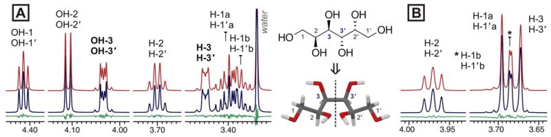
The 1H fingerprints of galactitol in different solvents. (A) NMR spectrum in DMSO-d6 (22 mM, 600 MHz); and (B) NOESY spectrum in water (12 mM, 10% D2O, pH 7.0, 600 MHz). The calculated and observed NMR spectra are shown in red and blue, respectively. Residuals are shown in green.
Although HiFSA profiles are inherently solvent-dependent, they can be used as foundation to build new profiles in different solvents. For instance, the HiFSA profile of galactitol in DMSO-d6 was used to explain the 1D NOESY spectrum in D2O (Figure 1B). The spectral parameters from DMSO-d6 were fitted to the NOESY spectrum and iterated, thereby creating a 1H fingerprint of galactitol in D2O despite extensive signal overlap in the 3.6–3.8 ppm region (Figure 1B).
The analysis of L-lysine demonstrated that HiFSA can provide a detailed description of spin systems containing multiple coupled methylenes (Figure 2A). HiFSA enabled the relative assignment of prochiral protons and the determination of coupling constants in signals that, otherwise, would be described as multiplets. As the identification of spectral patterns is essential in NMR-based metabolomic studies,22,23 the development of HiFSA profiles for endogenous metabolites will facilitate the NMR analysis of biofluids. Moreover, this approach can be used to refine an existing profile to consider variations in chemical shifts due to changes in analyte concentration, pH, and temperature (Figure 2B). The proposed assignments for L-lysine correspond to the best solution obtained by ACA, which not only yielded spectral parameters consistent with the molecular structure, but also exhibited the lowest root-mean squared deviation (rmsd) from the experimental results. Alternative solutions and their corresponding rmsd values are summarized in the Supporting Information.
Figure 2.

Comparison of two 1H fingerprints of L-lysine. (A) NMR spectrum (100 mM, 99.9% D2O, pH 7.4, 400 MHz); and (B) NOESY spectrum (5.5 mM, 10% D2O, pH 7.0, 500 MHz). The HiFSA profile of (A) was used to generate the profile of (B). The calculated spectra, observed spectra, and residuals are shown in red, blue, and green, respectively. (*) denotes impurity signals.
This example also indicates that HiFSA profiles can reproduce NMR spectra recorded at different field strengths. This concept was introduced by Tiainen et al., who used adaptive spectral libraries to simulate the NMR spectra of amino acid isotopomers.24 We extended these results by using the 600 MHz HiFSA profile of ginkgolide A25 to calculate the corresponding NMR spectrum at 60 MHz. Remarkably, the calculated low-field spectrum was in excellent agreement with the experimental data (Figure 3). This correlation between high-field spectra and calculated low-frequency fingerprints should have considerable applications in reaction and process monitoring.26,27
Figure 3.
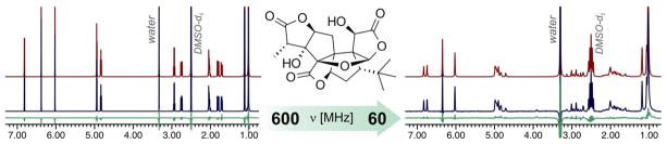
Simulation of NMR spectra of ginkgolide A in DMSO-d6 at different field strengths. Spectral parameters obtained at 600 MHz were used to calculate the NMR spectrum at 60 MHz. In both cases, excellent agreement between the calculated (red) and observed (blue) spectra was observed. Residuals are shown in green.
To test this approach on more complex molecules, a thorough spectral analysis of progesterone and atosiban was performed. Progesterone contains a spin network that comprises 23 protons and more than 40 coupling constants, including ubiquitous geminal and vicinal couplings (2,3J) and several long-range couplings (>4J) that are essential in the interpretation of the experimental data.28,29 The complex resonance patterns observed in the NMR spectrum, even at 900 MHz (Figure 4), were fully characterized using only the 1D 1H NMR data and a 2D 1H,1H–COSY experiment. This methodology enabled the assignment of all axial and equatorial protons in the ring system. Furthermore, HiFSA facilitated the analysis of distorted multiplets due to higher order effects (Figure 4). For instance, although H-9 (1.032 ppm) is affected by the strongly coupled protons H-11β and H-12α (1.519 and 1.504 ppm, respectively), all its δ and J values were readily determined (see Supporting Information).
Figure 4.
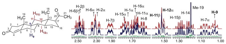
Sections of the calculated (red) and observed (blue) NMR spectra of progesterone (45 mM, methanol-d4, 900 MHz). Residuals are shown in green.
The analysis of atosiban demonstrates the characterization of individual amino acids in a moderately sized peptide. Semi-automated spectral analysis was carried out with ACA using the 1D 1H NMR spectrum and a 2D 1H,13C–HSQC experiment. Additional 2D NMR experiments (1H,1H–COSY and 1H,13C–HMBC) were used to verify all assignments, and the final optimization was carried out with the PERCH shell. As a result, HiFSA enabled the description of the NMR spectrum of atosiban, revealing the contribution of each constituent unit to the overall signal profile. HiFSA also facilitated the detection of impurities, including acetic acid and a structurally related peptide (Figure 5).
Figure 5.
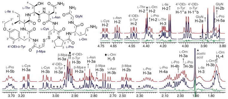
Sections of the calculated (red) and observed (blue) NMR spectra of atosiban (28 mM, methanol-d4, 600 MHz). Residuals are shown in green. (*) denotes impurity signals.
The examples described provide compelling evidence for the ability of HiFSA to resolve and fully assign individual resonances in complex NMR signal patterns. However, although the use of ACA is convenient, the automated analysis has limitations. Imperfections in the spectra (e.g., poor shimming or phasing) or sample impurities can affect the iteration process. Spectroscopic imperfections can be minimized by careful manual or gradient shimming and the use of proper post-acquisition processing such as that proposed for qHNMR analysis.30 While impurities may require specific attention, HiFSA is capable of addressing them both qualitatively and quantitative, as recently demonstrated for mixtures of natural products.6,31 Similarly, the success of automated assignment protocol relies on the accuracy of the spectral prediction. Using a database of fully analyzed experimental data, ACA takes into account averaging on the NMR time scale by mapping the conformational space and correlating conformational parameters. Therefore, HiFSA does not require iterative optimization of NMR parameters for each single conformer. As any method producing indirect structural evidence, ACA solutions must be reviewed to ensure that (i) an excellent fit is achieved; (ii) the assignments are correct; and (iii) the spectral parameters are consistent with the molecular structure.
A major strength of HiFSA fingerprinting is the ability to distinguish between closely related molecules, as recently shown for four silybin isomers with near-identical NMR spectra.31 Moreover, HiFSA profiles are stored in manageable, easy-to-share text files (2–20 kB in size). These profiles are especially suitable for rapid identification of known structures, with a broad range of applications for monitoring synthetic reactions and, as databases of HiFSA profiles pass critical size thresholds,32–34 for structural dereplication in natural product research. This approach also complements the information obtained from 2D NMR experiments in the characterization of new molecular entities, reducing the exploration of the configurational and conformational space to those structures compatible with the extracted spectral parameters. Moreover, as the recognition of characteristic 1H resonances becomes critical for mixture analysis in organic chemistry, forensic science, foodstuff quality assessment, and metabolomic research, the development of reproducible, digital NMR profiles will enable full exploitation of 1D 1H NMR for qualitative and quantitative analysis.
In summary, the computational approach described enhances the description of small molecules and generates highly reproducible 1H fingerprints, while it yields comprehensive NMR profiles including all assignments and spectral parameters. Overall, these profiles are highly descriptive and provide insight into the relative configuration and conformation of small molecules in solution, and ultimately represent a means of portraying molecular structures.
EXPERIMENTAL SECTION
Materials and Sample Preparation
High-purity analytes, deuterated solvents, and NMR tubes were obtained from commercial suppliers. All organic compounds were used as received without further purification. Samples for NMR analysis were prepared by precisely weighing 1–10 mg of the analyte in an analytical balance (±0.01 mg), followed by the addition of 600 μL of deuterated solvent. The samples were placed in a vortex mixer for 2 min to ensure complete dissolution as judged by visual inspection and transferred to 5-mm NMR tubes using gas-tight syringes. NMR spectra were recorded without sealing the NMR tubes, nor degassing the samples (see additional comments in the Supporting Information).
Molecular Structures
The 3D molecular structures of galactitol and L-lysine were built from scratch in PERCH’s MMS module. The structure of progesterone was obtained from its crystal structure bound to the human progesterone receptor (PDB ID: 1A28).35 The 3D molecular model of atosiban was generated with Maestro software (v.9.0.211) using the crystal structure of deamino-oxytocin as a template (PDB ID: 1XY2).36
NMR Spectroscopy
The 1D 1H NMR spectrum of L-lysine recorded in 99.9% D2O was downloaded from MMCD (http://mmcd.nmrfam.wisc.edu; entry: cq_00029; expnmr_00082). The 1D NOESY spectra of galactitol and L-lysine, acquired in water with 10% D2O and water presaturation, were downloaded from HMDB (http://www.hmdb.ca; ID: HMDB00107 and HMDB00182, respectively).
NMR measurements were recorded at 600.13 and 899.94 MHz (14.1 and 21.1 T static magnetic fields, respectively) on NMR spectrometers equipped with 5-mm, triple resonance inverse detection TXI and TCI cryoprobes, respectively. NMR experiments were acquired under temperature-controlled conditions at 298 K (25°C), and the probes were frequency tuned and impedance matched prior to each sample run. The 60 MHz 1H NMR spectrum of ginkgolide A was recorded on a permanent magnet NMR spectrometer operating at 60.01 MHz (1.4 T) with a dual channel (C/H) probe maintained at 303 K (30°C). Chemical shifts (δ) are expressed in ppm with reference to internal TMS or DSS (0.000 ppm). In cases when no internal reference is present, the residual solvent signal was used as reference. Scalar coupling constants (J) and effective linewidths (Δν½) are given in Hertz.
The 1D 1H NMR spectra were recorded under quantitative conditions using a 90° pulse experiment. The 90° pulse was calibrated by evaluating the null at 360° and back-calculating the corresponding pulse width. The following acquisition parameters were used: spectral width (sw) of 30 ppm, center of the spectral window (o1p) at 7.5 ppm, acquisition time (aq) of 4.0 s, and a relaxation delay (d1) of 60.0 s (more than five times the longest T1). For NMR experiments recorded at 900 MHz, eight transients were collected with 216,798 total data points, and a receiver gain of 64. NMR experiments at 600 MHz were recorded with 64 transients, 143,882 total data points, and a receiver gain of 16.
NMR data were processed with TopSpin software (v.3.2) or NUTS software (v.201004) using a Lorentz-to-Gaussian window function for resolution enhancement (line broadening = −0.3 Hz, Gaussian factor = 0.05). Zero filling was applied prior to Fourier transformation to increase the number of data points to 256K and 1024K in experiments recorded at 600 and 900 MHz, respectively. The resulting NMR spectra were subjected to manual phase adjustment and automatic baseline correction using polynomial functions.
The 2D NMR experiments were recorded at 600.13 MHz with 2K data points in F2 and 256 increments in F1. Magnitude-mode 1H,1H–COSY experiments were recorded using the following parameters: sw = 12 ppm in both F1 and F2, aq = 0.29 s in F2, and d1 = 1.0 s. Phase-sensitive 1H,13C–HSQC and 1H,13C–HMBC experiments were recorded with sw = 12 ppm in F2, aq = 0.29 s in F2, and d1 = 1.5 s. In HSQC and HMBC experiments, the spectral width in F1 was set to 170 and 220 ppm, respectively. In HMBC experiments, the inter-pulse delay for evolution of long-range heteronuclear coupling constants (d6) was set to 0.065 sec (i.e., 2,3JC,H = 7.7 Hz). Subsequent 2D NMR processing was carried out with TopSpin software. Zero filling was applied to both dimensions to obtain matrices of 4K × 4K spectral data points. After Fourier transformation, the 2D NMR experiments were phase-adjusted (if necessary) and baseline-corrected using polynomial functions.
Computer-aided NMR Spectral Analysis
Semi-automated NMR analysis was carried out with PERCH NMR tools (v.2011.1). The experimental NMR data (i.e., the 1D 1H NMR spectrum and, optionally, a 1D 13C NMR spectrum and/or a 2D 1H,13C–HSQC experiment) were imported into PERCH’s ACA module, together with the 3D molecular structure file (either in MDL Molfile format or prepared in PERCH’s MMS module). ACA performed the complete spectral analysis largely in automation. This process includes post-processing operations (peak picking and integration), conformational analysis, conformational sampling, and prediction of spectral parameters. Next, ACA evaluated potential solutions by fitting and honing the predicted spectral parameters of each solution against the observed 1H NMR spectrum using the QMTLS iterators. In cases where a consistent solution was not achieved in full automation (which is generally affected by spectral quality, molecular dynamics, purity, and overall complexity), the predicted spectral parameters were adjusted manually in the ACA-GUI or PERCH shell. The iteration process was then repeated until convergence was reached and the rmsd was ≤0.1%.
Supplementary Material
Acknowledgments
The authors acknowledge the vision and founding work of Dr. R. Laatikainen in establishing tools for QMTLS analysis. We also thank Dr. B. Ramirez for his assistance in the NMR facility at the UIC Center for Structural Biology (CSB), and Dr. A. Abe (Lake Forest College) for collecting the 60 MHz 1H NMR spectrum of ginkgolide A. This research work was funded by NIH through grant RC2 AT005899, awarded to Dr. G. F. Pauli by NCCAM. During the preparation of this manuscript, Dr. J. G. Napolitano was financially supported by the United States Pharmacopeial Convention through the 2012/2013 USP Global Fellowship Awards Program. The construction of the UIC CSB and the 900 MHz NMR spectrometer were funded by NIH through grant P41 GM068944, awarded to Dr. P. G. W. Gettins by NIGMS.
Footnotes
Contains spectral profiles and 1H NMR fingerprints. This material is available free of charge via the Internet at http://pubs.acs.org.
References
- 1.Abraham RJ. The Analysis of High Resolution NMR Spectra. Elsevier; Amsterdam: 1971. pp. 124–261. [Google Scholar]
- 2.Haigh CW. Annu Rep Nucl Magn Reson Spectrosc. 1971;4:311–362. [Google Scholar]
- 3.Abraham RJ, Mobli M. Modelling 1H NMR Spectra of Organic Compounds: Theory, Applications and NMR Prediction Software. Chapter 2. Wiley; Chichester: 2008. pp. 23–65. [Google Scholar]
- 4.Parr WJE, Schaefer T. Acc Chem Res. 1980;13:400–406. [Google Scholar]
- 5.Schaefer T. In: Encyclopedia of Magnetic Resonance (eMagRes) Harris RK, Wasylishen RE, editors. Wiley; Chichester: 2012. pp. 4726–4736. [Google Scholar]
- 6.Napolitano JG, Gödecke T, Rodríguez-Brasco MF, Jaki BU, Chen SN, Lankin DC, Pauli GF. J Nat Prod. 2012;75:238–248. doi: 10.1021/np200949v. [DOI] [PMC free article] [PubMed] [Google Scholar]
- 7.Laatikainen R, Niemitz M, Weber U, Sundelin J, Hassinen T, Vepsalainen J. J Magn Reson Ser A. 1996;120:1–10. [Google Scholar]
- 8.Laatikainen R, Niemitz M, Malaisse WJ, Biesemans M, Willem R. Magn Reson Med. 1996;36:359–365. doi: 10.1002/mrm.1910360306. [DOI] [PubMed] [Google Scholar]
- 9.Thiele H, McLeod G, Niemitz M, Kühn T. Monatsh Chem. 2011;142:717–730. [Google Scholar]
- 10.Laatikainen R, Tiainen M, Korhonen S-P, Niemitz M. In: Encyclopedia of Magnetic Resonance (eMagRes) Harris RK, Wasylishen RE, editors. Wiley; Chichester: 2011. pp. 1–12. [Google Scholar]
- 11.Boyd DB. In: Reviews in Computational Chemistry. Lipkowitz KB, Boyd DB, editors. Vol. 6. VCH Publishers; New York: 1995. pp. 317–354. [Google Scholar]
- 12.Hanwell MD, Curtis DE, Lonie DC, Vandermeersch T, Zurek E, Hutchison GR. J Cheminf. 2012;4:1–17. doi: 10.1186/1758-2946-4-17. [DOI] [PMC free article] [PubMed] [Google Scholar]
- 13.Allen FH. Acta Crystallogr, Sect B Struct Sci. 2002;B58:380–388. doi: 10.1107/s0108768102003890. [DOI] [PubMed] [Google Scholar]
- 14.Gražulis S, Chateigner D, Downs RT, Yokochi AFT, Quirós M, Lutterotti L, Manakova E, Butkus J, Moeck P, Le Bail A. J Appl Crystallogr. 2009;42:726–729. doi: 10.1107/S0021889809016690. [DOI] [PMC free article] [PubMed] [Google Scholar]
- 15.Berman HM, Westbrook J, Feng Z, Gilliland G, Bhat TN, Weissig H, Shindyalov IN, Bourne PE. Nucleic Acids Res. 2000;28:235–242. doi: 10.1093/nar/28.1.235. [DOI] [PMC free article] [PubMed] [Google Scholar]
- 16.Wishart DS, Tzur D, Knox C, Eisner R, Guo AC, Young N, Cheng D, Jewell K, Arndt D, Sawhney S, Fung C, Nikolai L, Lewis M, Coutouly MA, Forsythe I, Tang P, Shrivastava S, Jeroncic K, Stothard P, Amegbey G, Block D, Hau DD, Wagner J, Miniaci J, Clements M, Gebremedhin M, Guo N, Zhang Y, Duggan GE, MacInnis GD, Weljie AM, Dowlatabadi R, Bamforth F, Clive D, Greiner R, Li L, Marrie T, Sykes BD, Vogel HJ, Querengesser L. Nucleic Acids Res. 2007;35:D521–D526. doi: 10.1093/nar/gkl923. [DOI] [PMC free article] [PubMed] [Google Scholar]
- 17.Cui Q, Lewis IA, Hegeman AD, Anderson ME, Li J, Schulte CF, Westler WM, Eghbalnia HR, Sussman MR, Markley JL. Nat Biotechnol. 2008;26:162–164. doi: 10.1038/nbt0208-162. [DOI] [PubMed] [Google Scholar]
- 18.Ulrich EL, Akutsu H, Doreleijers JF, Harano Y, Ioannidis YE, Lin J, Livny M, Mading S, Maziuk D, Miller Z, Nakatani E, Schulte CF, Tolmie DE, Kent Wenger R, Yao H, Markley JL. Nucleic Acids Res. 2008;36:D402–D408. doi: 10.1093/nar/gkm957. [DOI] [PMC free article] [PubMed] [Google Scholar]
- 19.Ludwig C, Easton JM, Lodi A, Tiziani S, Manzoor SE, Southam AD, Byrne JJ, Bishop LM, He S, Arvanitis TN, Günther UL, Viant MR. Metabolomics. 2012;8:8–18. [Google Scholar]
- 20.Pence HE, Williams A. J Chem Educ. 2010;87:1123–1124. [Google Scholar]
- 21.Kalstabakken KA, Harned AM. J Chem Educ. 2013;90:941–943. [Google Scholar]
- 22.Verpoorte R, Choi YH, Kim HK. Phytochem Rev. 2007;6:3–14. [Google Scholar]
- 23.Lindon JC, Nicholson JK. Annu Rev Anal Chem. 2008;1:45–69. doi: 10.1146/annurev.anchem.1.031207.113026. [DOI] [PubMed] [Google Scholar]
- 24.Tiainen M, Maaheimo H, Niemitz M, Soininen P, Laatikainen R. Magn Reson Chem. 2008;46:125–137. doi: 10.1002/mrc.2140. [DOI] [PubMed] [Google Scholar]
- 25.Napolitano JG, Lankin DC, Chen SN, Pauli GF. Magn Reson Chem. 2012;50:569–575. doi: 10.1002/mrc.3829. [DOI] [PMC free article] [PubMed] [Google Scholar]
- 26.Edwards JC, Giammatteo PJ. In: Process Analytical Technology: Spectroscopic Tools and Implementation Strategies for the Chemical and Pharmaceutical Industries. 2. Bakeev KA, editor. Wiley; Chichester: 2010. pp. 303–335. [Google Scholar]
- 27.Dalitz F, Cudaj M, Maiwald M, Guthausen G. Prog Nucl Magn Reson Spectrosc. 2012;60:52–70. doi: 10.1016/j.pnmrs.2011.11.003. [DOI] [PubMed] [Google Scholar]
- 28.Kolehmainen E, Laihia K, Laatikainen R, Vepsalainen J, Niemitz M, Suontamo R. Magn Reson Chem. 1997;35:463–467. [Google Scholar]
- 29.Niemitz M, Laatikainen R, Chen SN, Kleps R, Kozikowski AP, Pauli GF. Magn Reson Chem. 2007;45:878–882. doi: 10.1002/mrc.2061. [DOI] [PubMed] [Google Scholar]
- 30.Pauli GF, Gödecke T, Jaki BU, Lankin DC. J Nat Prod. 2012;75:834–851. doi: 10.1021/np200993k. [DOI] [PMC free article] [PubMed] [Google Scholar]
- 31.Napolitano JG, Lankin DC, Graf TN, Friesen JB, Chen SN, McAlpine JB, Oberlies NH, Pauli GF. J Org Chem. 2013;78:2827–2839. doi: 10.1021/jo302720h. [DOI] [PMC free article] [PubMed] [Google Scholar]
- 32.Moco S, Tseng LH, Spraul M, Chen Z, Vervoort J. Chromatographia. 2006;64:503–508. [Google Scholar]
- 33.Roslund MU, Tähtinen P, Niemitz M, Sjöholm R. Carbohydr Res. 2008;343:101–112. doi: 10.1016/j.carres.2007.10.008. [DOI] [PubMed] [Google Scholar]
- 34.Roslund MU, Säwén E, Landström J, Rönnols J, Jonsson KHM, Lundborg M, Svensson MV, Widmalm G. Carbohydr Res. 2011;346:1311–1319. doi: 10.1016/j.carres.2011.04.033. [DOI] [PubMed] [Google Scholar]
- 35.Williams SP, Sigler PB. Nature. 1998;393:392–396. doi: 10.1038/30775. [DOI] [PubMed] [Google Scholar]
- 36.Wood SP, Tickle IJ, Treharne AM, Pitts JE, Mascarenhas Y, Li JY, Husain J, Cooper S, Blundell TL, Hruby VJ, Buku A, Fischman AJ, Wyssbrod HR. Science. 1986;232:633–636. doi: 10.1126/science.3008332. [DOI] [PubMed] [Google Scholar]
Associated Data
This section collects any data citations, data availability statements, or supplementary materials included in this article.