Statistical Properties of the Site-Frequency Spectrum Associated with Λ-Coalescents

Abstract

Statistical properties of the site-frequency spectrum associated with Λ-coalescents are our objects of study. In particular, we derive recursions for the expected value, variance, and covariance of the spectrum, extending earlier results of Fu (1995) for the classical Kingman coalescent. Estimating coalescent parameters introduced by certain Λ-coalescents for data sets too large for full-likelihood methods is our focus. The recursions for the expected values we obtain can be used to find the parameter values that give the best fit to the observed frequency spectrum. The expected values are also used to approximate the probability a (derived) mutation arises on a branch subtending a given number of leaves (DNA sequences), allowing us to apply a pseudolikelihood inference to estimate coalescence parameters associated with certain subclasses of Λ-coalescents. The properties of the pseudolikelihood approach are investigated on simulated as well as real mtDNA data sets for the high-fecundity Atlantic cod (Gadus morhua). Our results for two subclasses of Λ-coalescents show that one can distinguish these subclasses from the Kingman coalescent, as well as between the Λ-subclasses, even for a moderate (maybe a few hundred) sample size.

LARGE offspring number population models have recently been proposed as appropriate models with which to investigate high-fecundity natural populations. Some marine populations may belong to the class of high-fecundity populations, including Pacific oysters (Crassostrea gigas) (Beckenbach 1994; Li and Hedgecock 1998; Boudry et al. 2002), white sea bream (Diplodus sargus) (Planes and Lenfant 2002), and Atlantic cod (Gadus morhua) (Árnason 2004). Oysters feature in Williams (1975)’s elm and oyster model as an example of a high-fecundity population. Indeed, high-fecundity populations are discussed at length by Williams (1975) when comparing the benefits of sexual vs. asexual reproduction. Avise et al. (1988) compare genetic distances for mitochondrial (mt)DNA variation for three vertebrate species, american eels (Anguilla rostrata), hardhead catfish (Arius felis), and red-winged blackbirds (Agelaius phoeniceus), and conclude that historical effective population sizes may have been much lower than current census size. Low effective population size compared to census population size observed for certain marine populations in particular (e.g., Hedgecock et al. 1992), and reviewed by Hedgecock and Pudovkin (2011), may be evidence of high variance in offspring distribution. Indeed, Hedrick (2005) observes that low effective population size results from high variance in reproductive success in a population with large census size. High fecundity may also be a way for certain marine organisms with broadcast spawning to compensate for high mortality rate among juveniles, thus exhibiting type III survivorship curves.

Multiple-merger coalescent processes, so-called Λ- and Ξ-coalescents, arise naturally from large offspring number models (Donnelly and Kurtz 1999; Sagitov 1999, 2003; Möhle and Sagitov 2001; Eldon and Wakeley 2006; Sargsyan and Wakeley 2008; Birkner and Blath 2009; Huillet and Möhle 2011a). A key assumption to obtain a multiple-merger coalescent process from a large offspring number model is that the number of offspring of an individual can be up to the order of the population size with nonnegligible probability. In contrast to the classical Kingman coalescent framework, which has served as the standard null model in population genetics since its introduction (Kingman 1982), Λ-coalescents allow multiple instead of only binary collisions of ancestral lineages, in which the group of lineages coalescing in a given instance may include anywhere from two to all of the current active lineages. Selective sweeps (Durrett and Schweinsberg 2004, 2005; Coop and Ralph 2012), or large-scale spatial extinction and recolonization events (Barton et al. 2010, 2013), can also give rise to multiple-merger coalescent processes. In some cases, one naturally encounters the even more general Ξ-coalescents (Schweinsberg 2000), allowing simultaneous multiple mergers at a time, i.e., when distinct groups of ancestral lineages coalesce at the same time to distinct ancestors. Models of severe bottlenecks (Birkner et al. 2009) or diploidy (Möhle and Sagitov 2003) and recombination in conjunction with distinct loci can give rise to Ξ-coalescents. By way of example, a Ξ-coalescent admitting up to quadrifold simultaneous mergers is obtained from a diploid multilocus model with a skewed (high variance) offspring distribution (Birkner et al. 2013). Möhle and Sagitov (2001) provide a full mathematical classification of coalescent limits (as population size tends to infinity) of Cannings’ exchangeable population models.

The statistical methodology to test for the presence and particularities of the effects of multiple mergers, or to distinguish between different underlying Λ- and Ξ-coalescents within a family of models, is, however, still largely missing. Hedgecock and Pudovkin (2011) argue that large offspring number models are the right framework in which to study high-fecundity marine populations. Some large offspring number models (e.g., Sagitov 2003; Eldon and Wakeley 2006) introduce new parameters (coalescence parameters) determining the size and intensity of large offspring number events, i.e., when individuals have very many offspring. Estimating the coalescence parameters from genetic data may give us a way to distinguish between different population models. Indeed, Hedgecock and Pudovkin (2011) call for the development of such inference methods, in particular to infer parameters, to assess the quality of the estimators, and to construct hypothesis tests and confidence bounds.

On one hand are summary-statistics-based estimators for the parameter of certain classes of Λ-coalescents (Eldon 2011) in the infinite-sites model, such as the number of segregating sites, which may not represent a sufficient statistic, but are computationally efficient, and could be used to obtain prior information. On the other hand, there are full-likelihood-based point estimators, derived via relatively complex recursions—which are, in principle, amenable to Monte Carlo methods—taking all available information into account, but whose practical treatment becomes computationally prohibitive even for medium-sized data sets (Birkner and Blath 2008; Birkner et al. 2011). A small empirical simulation study for the latter can be found in Steinrücken (2009). For both types of estimators, an analysis of their statistical properties in the Λ case is still largely missing.

A summary statistic that contains much of the essential (in particular, topological) information of the underlying genealogical tree of the data is the site-frequency spectrum (SFS) (however, one may want to consult, e.g., Myers et al. 2008 for theoretical limitations). The spectrum is a key quantity when applying coalescent theory in inference; see, e.g., Wakeley (2007) for an overview and a discussion of the relation of the SFS with various other (simpler) summary statistics. The statistical properties of the SFS under the Kingman coalescent have been investigated in several studies (Fu 1995; Griffiths and Tavaré 1998; Živković and Wiehe 2008; Achaz 2009; Sainudiin et al. 2011). Extending in particular the results of Fu (1995) to Λ-coalescents is our aim. Recursions for the expected value, the variance, and the covariance of the number of derived mutations in the SFS are derived for a general Λ-coalescent.

Substantial theoretical research has been undertaken to identify the asymptotic behavior of the frequency spectrum associated with Λ-coalescents, culminating in the recent convergence results, as sample size tends to infinity, contained in Berestycki et al. (2013). However, so far it is not known how large samples need to be for the spectrum to be well approximated by the limiting asymptotic results of Berestycki et al. (2013) or, indeed, whether the approximation is equally good for all values of the relevant coalescent parameter. This question is addressed using simulations.

Finally, as an illustration we apply our methods to site-frequency spectra obtained for Atlantic cod (Árnason et al. 2000; Sigurgíslason and Árnason 2003; Árnason 2004) and fit Λ-coalescents to the data. The problem of distinguishing between coalescent classes by means of observing a realization of the SFS is also addressed using simulations.

Setup and Previously Known Results

Notation

A formal definition of the SFS is our starting point. We assume the infinitely many-sites model (Kimura 1969; Watterson 1975) of population genetics, where the genealogy of a sample of size n is described by an n-Λ-coalescent. Mutations occur at a rate θ/2 on the coalescent branches. Suppose further that we can distinguish between mutant and wild type, e.g., with the help of an outgroup. Then, the SFS of an n sample is given by

$${\xi }^{\left(n\right)}:=\left({\xi }_1^{\left(n\right)},\dots ,{\xi }_{n-1}^{\left(n\right)}\right),$$

where the ${\xi }_i^{\left(n\right)},i=1,\dots ,n-1$ denote the number of sites at which variants appear i times in our sample. The ${\xi }_i^{\left(n\right)}$ are also referred to as the number of derived mutations in i copies, when the ancestral state is known. The vector ξ⁽ⁿ⁾ is called the unfolded site-frequency spectrum of the n sample.

In the case where the ancestral state (variant) is unknown, one often considers ${\eta }_i^{\left(n\right)}={\xi }_i^{\left(n\right)}$ for i = 1, … , , which is the number of sites at which the less frequent variant (the minor allele) is present in i sequences, and := 1_{(n even)}n/2 + 1_{(n odd)}(n−1)/2, where 1_(A) = 1 if event A is true and zero otherwise. The observed polymorphisms become “few and far between” with corresponding small expected values as i increases, at least for the Atlantic cod data we investigate. Thus, for $i>\widehat{ı}$ for some suitable $\widehat{ı}$, we lump them together into one class labeled as ${\widehat{ı}}_{+}$. Considering only the first few classes and lumping the rest also speeds up the computations.

Then, ${\eta }^{\left(n\right)}:=\left({\eta }_1^{\left(n\right)},\dots ,{\eta }_{(n/2)}^{\left(n\right)}\right)$ is called the folded site-frequency spectrum of an n sample.

A Λ-coalescent is a partition-valued (one can think of enumerated DNA sequences and their ancestral relationships) exchangeable coalescent process determined by a finite measure Λ on [0, 1] (Donnelly and Kurtz 1999; Pitman 1999; Sagitov 1999). For a comprehensive overview see, e.g., Berestycki (2009). If there are currently n blocks in the partition (i.e., n active ancestral lineages), any particular set of k blocks merges into one at rate

$${\lambda }_{n,k}={\displaystyle {\int }_{\left[0,1\right]}{x}^{k-2}{\left(1-x\right)}^{n-k}\Lambda \left(dx\right)},\hspace{1em}k=2,\dots ,n.$$ (1)

Certain special cases of a Λ-coalescent include the following, some of which we use in our examples below:

• One recovers the Kingman coalescent for

  $$\Lambda \left(dx\right)={\delta }_0\left(dx\right),$$ (2)

• i.e. when the measure Λ is concentrated at the point 0.

• The Beta(2 − α,α)-coalescent (Schweinsberg 2003) is a Λ-coalescent characterized by the Λ-measure

  $$\Lambda \left(dx\right)=\frac{\Gamma \left(2\right)}{\Gamma \left(2-\alpha \right)\Gamma \left(\alpha \right)}{x}^{1-\alpha }{\left(1-x\right)}^{\alpha -1}dx,$$ (3)

• with α ∈ (0, 2), i.e., when the measure Λ is associated with the Beta-distribution with parameters 2 − α and α. The limiting case α = 2 (in the sense of weak convergence of measures) corresponds to the Kingman coalescent.

• Eldon and Wakeley (2006) considered purely atomic Λ-coalescents of the types

  $$\Lambda \left(dx\right)={\delta }_{\psi }\left(dx\right)$$ (4)
• and

  $$\Lambda \left(dx\right)=\frac{2}{2+{\psi }^2}{\delta }_0\left(dx\right)+\frac{{\psi }^2}{2+{\psi }^2}{\delta }_{\psi }\left(dx\right),$$ (5)

• with ψ ∈ [0, 1], where ψ = 0 gives the Kingman coalescent.

In the application examples that follow, we are mainly concerned with coalescents (3) and (4). Thus, the parameter α (1 < α ≤ 2) refers exclusively to coalescent (3), and the parameter ψ (0 < ψ < 1) to coalescent (4).

For α, we focus our attention on the parameter range 1 < α < 2, since this corresponds to Beta-coalescents that “come down from infinity”, i.e., admit a unique most-recent common ancestor even in the infinite-sample limit (Pitman 1999; Schweinsberg 2000). It can be argued whether this property is necessary from a biological point of view. However, our empirical results for real data sets yield so far only estimates of α between 1 and 2. In addition, the coalescent process derived from Schweinsberg’s (2003) population model converges to coalescent (3) only when 1 ≤ α < 2. For 0 < α < 1, the coalescent process is a discrete-time Ξ-coalescent (Schweinsberg 2003).

Related asymptotic results

In inference, one often relies on asymptotic results. The asymptotic behavior of the site- and allele-frequency spectrum of Λ-coalescents for (very) large sample sizes (as n → ∞), as well as related asymptotic results concerning the distributions of tree lengths or the “speed of coming down from infinity”, i.e., when the sample size is infinite (a mathematical peculiarity), how long it takes the ancestral lineages to become finite in number, is an active field of mathematical research. The concept of coming down from infinity may yet have real implications for inference. By way of example, the point-mass coalescent (4) does not come down from infinity, which implies that external branches become more dominating as sample size increases, regardless of the value of ψ. On the other hand, the Beta-coalescent (3) does come down from infinity, as does the Kingman coalescent.

Important asymptotic results regarding the SFS are obtained by Berestycki et al, (2013, Theorem 3), who provide convergence results (in the almost sure sense), as sample size tends to infinity, of the scaled SFS for an important class of Λ-coalescents, including the Beta-coalescent (3), as is now explained. We say that the measure Λ has (strong) α-regular variation at zero if

$$\Lambda \left(dx\right)=f\left(x\right)dx,\hspace{1em}\text{where}f\left(x\right)\sim A{x}^{1-\alpha }\text{as}x\to 0,$$

for some α ∈ (1, 2) and A > 0. This holds for the Beta(2 − α, α)-coalescent from (3). Then, the almost sure asymptotic behavior of each ${\xi }_i^{\left(n\right)}$ as n → ∞ is determined by the behavior of f(x) as x ↓ 0 for a large class of Λ-coalescents.

Theorem 1 (Berestycki et al. 2013). Assume that Λ has (strong) α-regular variation at zero for some 1 < α < 2 and A > 0. Then, for the site-frequency spectrum of an n sample, where the underlying genealogy is governed by a Λ-coalescent and mutation rate θ/2,

$$\begin{array}{c}\underset{n\to \mathrm{\infty }}{\text{lim}}\frac{{\xi }_i^{\left(n\right)}}{n^{2-\alpha }}=\frac{\theta }{2}{C}_{A,\alpha }\frac{\left(2-\alpha \right)\Gamma \left(i+\alpha -2\right)}{i!\Gamma \left(\alpha -1\right)}\\ =\frac{\theta }{2}{C}_{A,\alpha }\left(2-\alpha \right)\frac{\left(\alpha -1\right)\cdots \left(\alpha +i-3\right)}{i!},\end{array}$$

in the almost sure sense, for i = 1, … , n, where

$$C_{A,\alpha }=\frac{\alpha \left(\alpha -1\right)}{A\Gamma \left(2-\alpha \right)\left(2-\alpha \right)}.$$

We formulate Theorem 1 with a mutation rate θ/2 instead of θ as in Berestycki et al. (2013) to be consistent with Fu (1995) and other literature. The asymptotic results should be of direct relevance for us in the case of large sample sizes. However, the rate of convergence of the asymptotic results in terms of sample size n and the parameter α seems to be unresolved. The issue of rate of convergence is investigated below, using simulations.

From a statistical point of view an ideal result would be an (asymptotic) result for the joint distribution of the normalized SFS for general Λ-coalescents, and this may well soon be within reach. For the Kingman case, this has already been achieved: There is asymptotic normality for the joint distribution of tree lengths. Kersting and Stanciu (2013) obtain an asymptotic normality result for the scaled branch lengths associated with the Kingman coalescent, from which Kersting and Stanciu deduce that the asymptotic joint distribution of the frequency spectrum is independent Poisson.

As a partial analog, Kersting et al. (2013) prove convergence of the total length of external branches of the Beta-coalescent (3) in distribution to a stable random variable with index α. Their result indicates that the joint distribution of the branch lengths associated with a Λ-coalescent will not be asymptotically normal, but might instead be a multivariate stable distribution. However, the rate of convergence is not known in the results of Kersting et al. (2013).

The Expected Value, Variance, and Covariance of Derived Mutations in the SFS Associated with a Λ-Coalescent

In this section we compute the expected value $\mathbb{E}\left[{\xi }_i^{\left(n\right)}\right]$, the variance $\text{Var}\left({\xi }_i^{\left(n\right)}\right)$, and the covariance $\text{Cov}\left({\xi }_i^{\left(n\right)},{\xi }_j^{\left(n\right)}\right)$ of the SFS associated with Λ-coalescents. While exact solutions for a finite sample size n appear quite hard to obtain due to the multiple-merger property of Λ-coalescents, we derive recursions for these quantities. Fu (1995) (cf. Theorem S1 in Supporting Information) obtained closed-form expressions for these quantities when associated with the Kingman coalescent.

As above, let ${\xi }_i^{\left(n\right)}$ denote the random number of derived mutations in i copies in an n sample with mutation rate θ/2 and genealogy governed by a Λ-coalescent. Before stating our first result, we recall some simple properties of the block-counting process associated with a Λ-coalescent from Birkner and Blath (2008). The block-counting process (Y_t) simply counts the number of ancestral lineages present each time. Recall the corresponding rates λ_n,k from (1). When we refer to number of “leaves” (n), we mean the initial sample size. Thus, a “leaf” refers to one sampled (DNA) sequence. By using leaves rather than sequences we emphasize that we are thinking of the sequences as vertices in a graph describing the ancestral relations of the leaves. Let (Y_t)_t≥0 be the block-counting process of our Λ-coalescent, which is a continuous-time Markov chain on ℕ with jump rates

$$q_{ij}=\left(\begin{array}{c}i\\ i-j+1\end{array}\right){\lambda }_{i,i-j+1},\hspace{1em}i>j\ge 1.$$

The total jump rate away from state i is $-q_{ii}={\displaystyle {\sum }_{j=1}^{i-1}{q}_{ij}}$. By

$$p_{ij}:=\frac{q_{ij}}{-q_{ii}}$$ (6)

we denote the transition probabilities of the embedded discrete skeleton chain. Let

$$g\left(n,m\right):={\mathbb{E}}_n\left[{\displaystyle {\int }_0^{\mathrm{\infty }}{\mathbf{1}}_{\left(Y_s=m\right)}ds}\right]\hspace{1em}\text{for }\hspace{1em}n\ge m\ge 2$$ (7)

be the expected amount of time that Y_t, starting from n, spends in m. Decomposing according to the first jump of Y_t gives a recursion for g(n, m),

$$\begin{array}{l}g\left(n,m\right)={\displaystyle \sum _{k=m}^{n-1}{p}_{nk}g\left(k,m\right)},\hspace{1em}n>m\ge 2,\\ \text{and}\\ g\left(m,m\right)=\frac{1}{-q_{mm}},\hspace{1em}m\ge 2.\end{array}$$ (8)

The expected value $\mathbb{E}\left[{\xi }_i^{\left(n\right)}\right]$ of derived mutations

For 1 < k ≤ n, as in Fu (1995), an important quantity is the probability

$$p^{\left(n\right)}\left[k,b\right],\hspace{1em}\text{for }b\in \left\{1,\dots ,n-\left(k-1\right)\right\},$$

that in a Λ-coalescent starting from n leaves, conditioned that there are at some point in time exactly k branches, a given one of these k branches (e.g., the first, if we think of some ordering) subtends exactly b leaves (see Figure 1).

Figure 1.

Illustration of the occurrence of an event with probability p⁽ⁿ⁾[k, b], with k = 2, and 2 ≤ b = n − 3. Ancestral lineage labeled as (2, 1), present when there are only two active ancestral lineages, is ancestral to b leaves (b sampled sequences). In this example, the first merger in the genealogical history of the n leaves is a 3 merger not involving any of the encircled b leaves. The second event is a b merger with b edges subtending the encircled b leaves merging to block (2, 1) (square). A “level” refers to the values of the lineage-counting process Y_t.

A recursion for p⁽ⁿ⁾[k, b] (Equation A2), given in the Appendix (Proposition A1), can be solved numerically, separately for each k. Equation (A2) allows us to derive a recursion for the expected frequency spectrum associated with Λ-coalescents, given in the following proposition.

Proposition 1. Under the above assumptions, we have, for i = 1, … , n − 1,

$$\mathbb{E}\left[{\xi }_i^{\left(n\right)}\right]=\frac{\theta }{2}{\displaystyle \sum _{k=2}^{n-i+1}{p}^{\left(n\right)}\left[k,i\right]\cdot k\cdot g\left(n,k\right)}.$$

The proof proceeds by decomposing according to the “level” (the values taken by the lineage-counting process Y_t) of the coalescent tree where a mutation arises—see the Appendix for details. Proposition 1 and its proof are a natural extension of the arguments of Griffiths and Tavaré (1998) to the multiple-merger case.

The expression in Proposition 1 can be used to define a quantity (ϕ_n(i)), the “expected normalized frequency spectrum”, which describes the shape of the genealogy and does not depend on θ, as follows. Let $B_i^{\left(n\right)}$ denote the random total length of branches subtending i leaves, for 1 ≤ i < n. Then, clearly, $\mathbb{E}\left[{\xi }_i^{\left(n\right)}\right]=\left(\theta /2\right)\mathbb{E}\left[B_i^{\left(n\right)}\right]$, with

$$\mathbb{E}\left[B_i^{\left(n\right)}\right]={\displaystyle \sum _{k=2}^{n-i+1}{p}^{\left(n\right)}\left[k,i\right]\cdot k\cdot g\left(n,k\right).}$$

If we now let B⁽ⁿ⁾ denote the random total length of the genealogy started from n leaves, and by ${\xi }^{\left(n\right)}={\xi }_1^{\left(n\right)}+.\hspace{0.17em}.\hspace{0.17em}.+{\xi }_{n-1}^{\left(n\right)}$ we denote the random total number of segregating sites in a sample of size n gene copies (DNA sequences), we have

$$\mathbb{E}\left[{\xi }^{\left(n\right)}\right]=\left(\theta /2\right)\mathbb{E}\left[B^{\left(n\right)}\right].$$

If T_ℓ denotes the random time during which there are ℓ active lineages, for 2 ≤ ℓ ≤ n, we have

$$\mathbb{E}\left[B^{\left(n\right)}\right]={\displaystyle \sum _{\ell =2}^n\ell \mathbb{E}\left[T_{\ell }\right].}$$

We define ϕ as

$${\varphi }_n\left(i\right):=\frac{\mathbb{E}\left[{\xi }_i^{\left(n\right)}\right]}{{\displaystyle {\sum }_{\ell =2}^n\ell \mathbb{E}\left[T_{\ell }\right]}}=\frac{{\displaystyle {\sum }_{k=2}^{n-i+1}{p}^{\left(n\right)}\left[k,i\right]\cdot k\cdot g\left(n,k\right)}}{{\displaystyle {\sum }_{\ell =2}^n\ell g\left(n,\ell \right)}}.$$ (9)

Loosely speaking, the probability that a mutation, under the infinitely many-sites assumption (Kimura 1969; Watterson 1975), with known ancestral types, appears i times in a sample of size n is ϕ_n(i). The quantity ϕ_n(i) is a quotient of expectations that can be interpreted as size biasing—it should not be confused with averaging over the quotient of these quantities, e.g., obtained from an empirical study, which has a different interpretation and will, at least for finite sample sizes, take different values. However, one can apply ϕ_n(i) as the main ingredient in a pseudolikelihood approach to infer coalescence parameters, as we do below.

The covariance $\text{Cov}\left({\xi }_i^{\left(n\right)},{\xi }_j^{\left(n\right)}\right)$ of derived mutations

To compute covariances one needs to compute the probability that two edges (ancestral lineages) drawn at random without replacement (ordered sampling) from the past, say from Y-states k and ℓ ≤ n, produce i (resp.) j subtended leaves. To this end, we need to distinguish three situations, namely whether our two edges are taken from the same “layer” (that is, when Y is in the same state k for both edges) or, if this is not the case, whether one of our two edges is a descendant of the other (“nested case”) or not (“unnested case”). In our calculations the leaves are unlabeled.

Case 1: Two edges in the same layer:

For 2 ≤ k ≤ n let $p_{\text{eq}}^{\left(n\right)}\left[k;i,j\right]$ be the probability that in an n-Λ-coalescent, conditioned on there being k ≥ 2 ancestral lineages at some time in the past, if we draw two of the k lines at random without replacement from these k (ordered sample), the first drawn line has i and the second j subtended leaves (see Figure 2). A recursion for $p_{\text{eq}}^{\left(n\right)}$ (Proposition A2) and proof are given in the Appendix.

Figure 2.

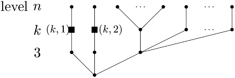
Illustration of the occurrence of the event with probability $p_{\text{eq}}^{\left(n\right)}\left[k;i,j\right]$ with i = j = 1. The ancestral lines (k, 1) and (k, 2) are each ancestral to one leaf. Level k is reached in one n − k + 1 merger not involving the two leaves subtended by (k, 1) or (k, 2).

Case 2: Two edges in different layers, unnested case:

For 2 ≤ k < ℓ ≤ n let $p_{\text{un}}^{\left(n\right)}\left[k,i;\ell ,j\right]$ be the probability that in an n-Λ-coalescent, conditioned on there being k lines at some time in the past and ℓ lines at some (other) time in the past, if we draw one of the k lines at random and independently one of the ℓ lines at random (ordered sample), the first drawn line has i and the second j subtended leaves, and the second is not a descendant of the first (see Figure 3). A recursion for $p_{\text{un}}^{\left(n\right)}$ (Proposition A3) is obtained in a similar way to that for $p_{\text{eq}}^{\left(n\right)}$, and is given in the Appendix along with a proof.

Figure 3.

Illustration of the occurrence of the event with probability $p_{\text{un}}^{\left(n\right)}\left[k,i;\ell ,j\right]$. Edge (ℓ, 1) in level ℓ subtends j leaves, while edge (k, 1) in level k subtends i leaves; 2 ≤ k < ℓ ≤ n, and the two encircled groups of i and j leaves are distinct. Level ℓ is reached in one merger including all of the j leaves. The following merger includes all of the i leaves.

Case 3: Two edges in different layers, nested case:

For 2 ≤ k < ℓ ≤ n let $p_{\text{ne}}^{\left(n\right)}\left[k,i;\ell ,j\right]$ be the probability that in an n-Λ-coalescent, conditioned on there being k lines at some time in the past and ℓ > k lines at some more recent time in the past, if we draw (ordered sample) one of the k lines at random [(k, 1), say, see Figure 4] and independently one of the ℓ lines [(ℓ, 1), say, see Figure 4] at random, the first drawn line has i and the second j subtended leaves, and the second (ℓ, 1) is a descendant of the first [(k, 1), so necessarily i ≥ j, and otherwise the probability is zero; see Figure 4]. The recursion for $p_{\text{ne}}^{\left(n\right)}$ is given in Proposition A4 in the Appendix, with the proof following similar arguments to proofs of Propositions A2 and A3.

Figure 4.

Illustration of the occurrence of the event with probability $p_{\text{ne}}^{\left(n\right)}\left[k,i;\ell ,j\right]$. Edge (ℓ, 1) in level ℓ subtends the encircled subset of j leaves, while edge (k, 1) in level k subtends (ℓ, 1) and the larger encircled set of i leaves necessarily containing the set of j leaves.

Unfortunately, the computational complexity of the recursions for $p_{\text{eq}}^{\left(n\right)}$ (Equation A4), $p_{\text{un}}^{\left(n\right)}$ (Equation A6), and $p_{\text{ne}}^{\left(n\right)}$ (Equation A8), as they stand, is O(n⁵), thus restricting numerical computations to relatively small values of n.

Second moments and covariance of the frequency spectrum:

Now we can put our recursions for $p_{\text{eq}}^{\left(n\right)}$, $p_{\text{un}}^{\left(n\right)}$, and $p_{\text{ne}}^{\left(n\right)}$ together to obtain the covariances $\text{Cov}\left({\xi }_i^{\left(n\right)},{\xi }_j^{\left(n\right)}\right)$. Our main result on the site-frequency spectrum associated with Λ-coalescents, an expression for $\mathbb{E}\left[{\xi }_i^{\left(n\right)}{\xi }_j^{\left(n\right)}\right]$ in terms of $p_{\text{eq}}^{\left(n\right)}$, $p_{\text{un}}^{\left(n\right)}$, $p_{\text{ne}}^{\left(n\right)}$, p⁽ⁿ⁾[k, i], and g(n, m), is now stated—a proof is in the Appendix.

Theorem 2. For 1 ≤ i, j < n, 2 ≤ i + j ≤ n, we have

$$\begin{array}{l}\mathbb{E}\left[{\xi }_i^{\left(n\right)}{\xi }_j^{\left(n\right)}\right]\\ =\frac{{\theta }^2}{4}{\displaystyle \sum _{k=2}^{n}k\left(k-1\right)p_{\text{eq}}^{\left(n\right)}\left[k;i,j\right]\frac{g\left(n,k\right)}{g\left(k,k\right)}\frac{2}{{\left(-q_{kk}\right)}^2}}\\ +\hspace{0.5em}{\mathbf{1}}_{(i=j)}{\displaystyle \sum _{k=2}^{n}k{p}^{\left(n\right)}\left[k,i\right]\frac{g\left(n,k\right)}{g\left(k,k\right)}\left(\frac{\theta }{2}\frac{1}{-q_{kk}}+\frac{{\theta }^2}{4}\frac{2}{{\left(-q_{kk}\right)}^2}\right)}\\ +\hspace{0.5em}\frac{{\theta }^2}{4}{\displaystyle \sum _{k=3}^n{\displaystyle \sum _{\ell =2}^{k-1}k\hspace{0.17em}{k}^{\prime }}}\\ \cdot \hspace{0.5em}\frac{p_{\text{un}}^{\left(n\right)}\left[k,i;\ell ,j\right]+p_{\text{ne}}^{\left(n\right)}\left[k,i;\ell ,j\right]+p_{\text{un}}^{\left(n\right)}\left[k,j;\ell ,i\right]+p_{\text{ne}}^{\left(n\right)}\left[k,j;\ell ,i\right]}{\left(-q_{kk}\right)\left(-q_{\ell \ell }\right)}\\ \cdot \hspace{0.5em}\frac{g\left(n,\ell \right)}{g\left(\ell ,\ell \right)}\frac{g\left(\ell ,k\right)}{g\left(k,k\right)}.\end{array}$$

In Figure 5 and Figure 6 we graph the covariances (Equation A17) of the branch lengths $B_i^{\left(n\right)}$ and $B_j^{\left(n\right)}$, where $B_i^{\left(n\right)}$ denotes the total length of branches subtending i of n leaves, and the coalescent process is the Beta(2−α, α)-coalescent. The variances and covariances become completely dominated by the variance of the length of external branches when multiple mergers are more prominent in the genealogy, i.e., when α is close to 1 (Figure 5). This means that the variances and covariances of the SFS will be dominated by the variance in the number of singletons, when associated with Λ-coalescents, and multiple mergers dominate the genealogy, as would occur in a high-fecundity population with frequent occurrence of large offspring number events. In the Beta-coalescent (Equation 3), large offspring number events become more prominent as α approaches 1 and less prominent as α approaches 2. And even when α is more “modest” at 1.5, the covariances are still quite small compared to the variances. Figure 6 shows the covariances on their own scale, i.e., with the variances and the diagonal covariances $\text{Cov}\left(B_i^{\left(n\right)},B_{n-i}^{\left(n\right)}\right)$ set at zero. These results suggest that one may model the site-frequency spectrum of an n-Λ-coalescent as composed of uncorrelated (but not independent) components ${\xi }_i^{\left(n\right)}$ for n large enough.

Figure 5.

The covariance $\text{Cov}\left(B_i^{\left(n\right)},B_j^{\left(n\right)}\right)\left(C\right)$ for sample size n = 40 for the Beta(2 − α, α)-coalescent with α as shown. The bottom panels show only the covariance terms, with the variance terms $\text{Var}\left(B_i^{\left(n\right)}\right)$ set equal to zero. The covariances range between −0.094 and 14.85 when α = 1.05 and between −0.045 and 2.06 when α = 1.5. One has $\text{Cov}\left({\xi }_i^{\left(n\right)},{\xi }_j^{\left(n\right)}\right)=\left({\theta }^2/4\right)\text{Cov}\left(B_i^{\left(n\right)},B_j^{\left(n\right)}\right)$ for i ≠ j, and $\text{Var}\left({\xi }_i^{\left(n\right)}\right)=\left(\theta /2\right)\mathbb{E}\left[B_i^{\left(n\right)}\right]+\left({\theta }^2/4\right)\text{Var}\left(B_i^{\left(n\right)}\right)$.

Figure 6.

The covariance $\text{Cov}\left(B_i^{\left(n\right)},B_j^{\left(n\right)}\right)$ (C) for sample size n = 40 for the Beta(2 − α, α)-coalescent with α as shown and with covariances $\text{Cov}\left(B_i^{\left(n\right)},B_{n-i}^{\left(n\right)}\right)$ and the variance terms set equal to zero.

For fixed n, the covariances between $B_i^{\left(n\right)}$ and $B_{n-i}^{\left(n\right)}$ seem to be larger than the covariances off the diagonals. As for the Kingman case, this can be explained by considering the first branching event in the coalescent history forward in time after the root. This has substantial probability to be a binary split, say in subfamilies of size i and n − i, which yields a positive correlation between $B_i^{\left(n\right)}$ and $B_{n-i}^{\left(n\right)}$.

Extending our results to the case of Ξ-coalescents and multiple loci is a natural follow-up task, but lies beyond the scope of the current discussion and will be part of future research.

Simulation Studies and Data Analysis

Reliability of the asymptotic results of Berestycki et al. (2013)

The asymptotic results obtained by Berestycki et al. (2013) (see Theorem 1) can be used to obtain estimates of α provided the asymptotic results are “close” to the true value and one has an estimate of θ. Ideally, such inference should take into account correlation between loci. Now we address the question of how large the sample must be for the SFS to be well approximated by the asymptotic results of Berestycki et al. (2013) and, indeed, whether one can trust the asymptotic results for all values of α.

Figure 7 compares the asymptotic results in Theorem 1 to simulated values for sample size n = 500 (left column) and n = 1000 (right column) and with α varying as shown. Even though we have recursions to obtain the exact expected values for finite n, we were not able, with present computer power, to compute covariances for n ≥ 100. The estimated expected values and the ones from the recursions are in agreement (results not shown). Even for n = 10⁴ (Figure 1 and Figure 2), which would be a rather large sample, the asymptotic results (Figure 7, shaded bars) match the simulated ones (Figure 7, open bars) rather poorly when α < 1.5, but the correspondence improves as α increases, and at α = 1.5 the match is already quite good. For more common sample sizes n ≤ 10³ (Figure 3 and Figure 7) the match is not very good for α ≤ 1.5. Relying on asymptotic results to estimate α might thus give misleading results, even when sample size is quite large, as demonstrated in Figure 8, which compares the asymptotic results for the singletons to the scaled (with n^α−2) exact expected values as sample size n and α vary as shown. The poor fit of the asymptotic results to exact values of the SFS, at least for lower values of α, suggests that exact results for the SFS, if only in the form of recursions, may be a better choice for inference methods.

Figure 7.

The results of Berestycki et al. (2013) (Theorem 1) regarding convergence of the scaled unfolded frequency spectrum (shaded bars) compared to simulations (open bars) varying over α as shown, with θ = 1. The left column is for sample size n = 100, and the right column is for sample size n = 250. The whiskers represent standard deviation.

Figure 8.

The asymptotic results of Berestycki et al. (2013) (Theorem 1) for the scaled singletons (lines) compared to the corresponding scaled exact expected values (symbols) as a function of sample size n ∈ {10, 20, 50, 100, 200, 300, 500, 1000, 2000, 10,000} on log-scale and varying over α as shown. Thus, the solid line and circles refer to α = 1.05, the short-dashed line and squares refer to α = 1.25, and so on.

Inference Methods and Data Analysis

Before we discuss our results on the analysis of the Atlantic cod data, we introduce our two inference methods, comparing observed and expected values using an ℓ² distance and a pseudolikelihood approach.

The ℓ² distance

The simplest way to find a value of α or ψ that gives the best fit to the data would be to compare the expected values of the frequency spectrum to the observed one and report the parameter value that minimizes the sum of squares (Equation 10). To avoid having to jointly estimate the mutation rate, we can define the scaled frequency spectrum ${\zeta }_i^{\left(n\right)}$ as

$${\zeta }_i^{\left(n\right)}:=\frac{{\eta }_i^{\left(n\right)}}{{\displaystyle {\sum }_{i=1}^{\lfloor n/2\rfloor }{\eta }_i^{\left(n\right)}}}.$$

The observed ${\zeta }_i^{\left(n\right)}$ are compared to the ratio of expected values

$$r_i^{\left(n\right)}:=\frac{\mathbb{E}\left[{\eta }_i^{\left(n\right)}\right]}{{\displaystyle {\sum }_{i=1}^{\lfloor n/2\rfloor }\mathbb{E}\left[{\eta }_i^{\left(n\right)}\right]}}.$$

Although clearly one should compare ${\zeta }_i^{\left(n\right)}$ to its actual expected value, simulation results indicate that our approximation is quite good (results not shown). A natural distance measure to compare ${\zeta }_i^{\left(n\right)}$ and $r_i^{\left(n\right)}$ is the ℓ² distance

$${\ell }^2=\sqrt{{\displaystyle \sum _{i=1}^{n/2}{\left({\zeta }_i-r_i\right)}^2}}.$$ (10)

A similar distance measure is the G_ξ statistic proposed by Fu (1996), in which each term in the sum is weighted by the variance of ${\xi }_i^{\left(n\right)}$ $\left({\eta }_i^{\left(n\right)}\right)$. The computational cost of computing the variances for a Λ-coalescent prevents us from considering an identical statistic for Λ-coalescents. A drawback of Fu’s (1996) G_ξ statistic is that it depends on the mutation rate θ. Ideally, one would want to apply a statistic that did not depend on θ. Instead, a statistic that reflects the underlying genealogy is desirable, since the processes that one usually tries to learn about in population genetics affect the topology and the branch lengths of the genealogy of a sample in one way or another. Determining statistical significance levels of the ℓ² distance is postponed for now; however, one may apply the approach of Fu (1996) to determine significance levels and statistical power.

The pseudolikelihood approach

A more fundamental statistical inference procedure than simply applying the ℓ² statistic is a likelihood inference. Ideally, in our case, to construct a likelihood function, one would have a way of writing down the probability of observing a mutation i times in a sample in terms of the coalescence parameters. However, these probabilities depend on the coalescence parameters in a way that is hard to make explicit, and therefore we approximate them with the quantity ϕ_n(i) (Equation 9). We interpret the observed site-frequency spectrum as an observation from a multinomial distribution, in which the probability of each class is estimated using ϕ_n(i). For 1 ≤ i < n, ϕ_n(i) is the expected number of mutations in i copies scaled by the expected total number of segregating sites, which corresponds to the expected total number of branches subtending i leaves scaled by the expected total size of the genealogy. Since we can compute ϕ_n(i) only numerically, Fisher information cannot be computed easily, and it would not be a priori clear whether the variance and confidence bounds derived therefrom via classical statistical theory would be valid. Finally, we refer to our likelihood approach as a pseudolikelihood inference.

Now we state our pseudolikelihood function. Let s denote the total number of segregating sites, and let s = (s₁, … , s_k, $s_{k_{+}}$) be the observed folded frequency spectrum, where $s_{k_{+}}$ denotes the collapsed class. Write ϕ_i := ϕ_n(i), and define ${\varphi }_{k_{+}}=1-{\varphi }_1-\dots -{\varphi }_k$. The pseudolikelihood function L_s(π) takes a multinomial form, in which π denotes the appropriate coalescence parameter (ψ or α):

$${\mathit{L}}_{\mathbf{s}}\left(\pi \right)=\left(\begin{array}{c}s\\ s_1\dots \hspace{0.17em}{s}_k{s}_{k_{+}}\end{array}\right){\varphi }_1^{s_1}\dots \hspace{0.17em}{\varphi }_k^{s_k}{\varphi }_{k_{+}}^{s_{k_{+}}}.$$ (11)

The form of L can be seen from the way we view the data s: as an observation from a multinomial distribution in which the probability of each class is estimated with ϕ_i. It suffices to consider the pseudo-log-likelihood function

$${\mathit{l}}_{\mathbf{s}}\left(\pi \right)=s_1 \log \left({\varphi }_1\right)+\dots +s_{k_{+}}\log \left({\varphi }_{k_{+}}\right).$$

As in the case of the statistics ${\zeta }_i^{\left(n\right)}$ and $r_i^{\left(n\right)}$, this pseudolikelihood approach does not require an estimate of θ. In Table 1 we do show that the pseudolikelihood performs as it should, when applied to the expected site-frequency spectrum of different coalescent processes.

Table 1. Pseudo-log-likelihood values and maximum-likelihood estimates ($\widehat{\alpha }$ and $\widehat{\psi }$) of coalescent parameters α and ψ for the pseudolikelihood (11) with $p_i:=\mathbb{E}\left[{\mathit{B}}_{\mathit{i}}^{\left(n\right)}\right]/\mathbb{E}\left[B^{\left(n\right)}\right]$.

n	π	$\widehat{\alpha }$	$\widehat{\psi }$	$\log L\left(\widehat{\alpha }\right)$	$\log L\left(\widehat{\psi }\right)$	log L(0)
10	0	1.96	0.02	−5.404	−5.405	−5.404
100		1.96	0.02	−19.027	−19.176	−19.021
1000		1.96	0.02	−38.868	−43.281	−38.847
10	1.05	1.06	0.30	−5.122	−5.159	−5.583
100		1.06	0.12	−26.179	−27.483	−35.3964
1000		1.04	0.04	−106.80	−120.525	−204.1335
10	1.5	1.50	0.14	−5.410	−5.419	−5.508
100		1.50	0.04	−23.731	−24.163	−25.272
1000		1.50	0.02	−71.143	−78.175	−81.3238
10	0.01	1.96	0.02	−54,110.92	−54,113.630	−54,113.59
100		1.90	0.02	−194,644.8	−194,884.834	−194,951.4
1000		1.62	0.02	−440,572.40	−432,453.967	−466,074.3
10	0.5	1.02	0.5	−19.219	−18.378	−23.28243
100		1.02	0.5	−85.749	−63.553	−207.8592
1000		1.02	0.5	−329.189	−130.413	−2,099.191

By L(0) we denote the log-likelihood associated with the Kingman coalescent. Data are the expected unfolded frequency spectrum associated with a particular coalescent with parameter π. Values associated with the Λ_ψ-coalescent (Equation 4) were computed for the range [0.02, 0.96], and those for Λ_α (Equation 3) in the range [1.02, 1.96]. One computes $\text{log}L\left(0\right)={\displaystyle {\sum }_{i=1}^{n-1}\left(1/i\right)\text{log}\left(\left(2/i\right)/\mathbb{E}\left[L_K\right]\right)}$, $\mathbb{E}\left[L_K\right]=2{\displaystyle {\sum }_{i=1}^{n-1}1/i}$.

Table 1 shows maximum-likelihood estimates of the coalescence parameters α and ψ, when the data are the expected values of the site-frequency spectrum, obtained for given values of the appropriate coalescent parameter, denoted by π in Table 1 and computed using our recursion (Proposition 1). Thus, π = α when π ∈ (1, 2) and π = ψ when π ∈ (0, 1). For each combination of sample size n and π, the log-likelihood values are compared with the ones obtained for the Kingman coalescent log L(0). Highest log-likelihood values are always obtained for the correct parameter value even for sample size n as low as 10. And for modest sample sizes, one should be able to correctly identify the Kingman coalescent (π = 0 in Table 1).

In Figures 14–16 in supporting information, File S1, we estimate the distribution of the maximum-likelihood estimator for different values of n, θ, and the coalescence parameters α and ψ. As one expects, the performance of the pseudolikelihood is better for larger values of n and θ.

A natural question to address is, How well do the probabilities ϕ_n(i) (Equation 9) actually fit with the correct values $\mathbb{E}\left[{\zeta }_i^{\left(n\right)}\right]$? In Figures 5 and 6 in File S1 we address this issue via simulations. The agreement between p_i and $\overline{R_i}$ is best when the number n of leaves (sample size) is large and α is closer to 2 than to 1.

The C code written to carry out the computations is available upon request.

Atlantic cod mtDNA data analysis

An application of the recursion (Proposition 1) for the exact expected values for the site-frequency spectrum is now illustrated using data on Atlantic cod obtained from various localities in the North Atlantic (Árnason et al. 2000; Sigurgíslason and Árnason 2003; Árnason 2004). The shallow gene genealogies observed among the haplotypes sampled, coupled with very high fecundity of Atlantic cod, led Árnason (2004) to argue that the Kingman coalescent may not be an appropriate null model for Atlantic cod. Later studies (Eldon 2011; Steinrücken et al. 2013) support that conclusion by finding a better match between the data and the Beta-coalescent than obtained for the Kingman coalescent. Eldon (2011) employ the asymptotic results of Berestycki et al. (2013) on the site-frequency spectrum obtained from Árnason (2004), while Steinrücken et al. (2013) employ full-likelihood methods on the sequence data of Atlantic cod data sets of smaller size than in Árnason (2004).

The Atlantic cod mtDNA data sets we analyze are summarized in Table 2. The sequence data from the Faroe Islands (Sigurgíslason and Árnason 2003) consist of a 250-bp segment from the mitochondrial cytochrome b gene in addition to 242- and 74-bp segments for a total of 566 bp. The data from Greenland and Iceland described in Árnason et al. (2000) consist of the 250-bp segment and so do the combined data described in Árnason (2004).

Table 2. The folded frequency spectrum for the Atlantic cod data in Árnason et al. (2000), Sigurgíslason and Árnason (2003), and Árnason (2004).

Source	s	η1	η2	η3	η4	η5	η6	η7	η8	η9	η10	η11+
Árnason et al. (2000)
Greenland (78)	9	3	1	0	1	0	0	1	1	1	0	1
Iceland (519)	23	12	1	4	1	0	0	0	0	0	0	5
Joint (597)	24	11	3	3	1	1	0	0	0	0	0	5
Sigurgíslason and Árnason (2003)
Faroe Islands (74)	44	23	9	1	1	1	0	9	0	0	0	0
Árnason (2004) (1278)	39	17	4	4	2	4	1	0	1	0	0	6

The sample size of each data set is given in parentheses. Mutations of frequency classes from 11 onward are lumped together in the 11+ class except for the data from Faroe Islands, in which mutations from 7 onward are lumped into the 7+ class. The symbol s denotes the total number of segregating sites.

In Figure 9 and Figure 10 the ℓ² distances comparing ${\zeta }_i^{\left(n\right)}$ and $r_i^{\left(n\right)}$ obtained for the different Atlantic cod data sets are compared. The corresponding parameter estimates are reported in Table 3. For the larger data sets one observes much “sharper” curves than for the smaller ones as one would expect, since the larger data sets carry more information. The difference in ℓ² distance between the coalescent processes is also biggest for the larger data sets, with the Beta-coalescent showing the best fit for all the data sets, although the difference between the two Λ-coalescents is not always large. However, based on this simple parameter estimation method, one would clearly prefer one of the two Λ-coalescents over the Kingman coalescent.

Figure 9.

The ℓ² distance between ζ_i and r_i for the five different Atlantic cod data sets, with expected values obtained for the Beta-coalescent. The values associated with the Kingman coalescent are obtained for α = 2. The A04 data set refers to the one in Árnason (2004).

Figure 10.

The ℓ² distance between ζ_i and r_i for the five different Atlantic cod data sets, with expected values obtained for the point-mass coalescent. See Figure 9 for explanation of symbols.

Table 3. The parameter values minimizing the ℓ² distance.

Data	$\widehat{\alpha }$	$\widehat{\psi }$	${\ell }^2\left(\widehat{\alpha }\right)$	${\ell }^2\left(\widehat{\psi }\right)$	ℓ2(0)
Faroe Islands	1.35	0.084	0.113	0.165	0.371
Greenland (G)	1.65	0.036	0.200	0.217	0.272
Iceland (I)	1.45	0.022	0.154	0.172	0.473
G + I	1.50	0.016	0.077	0.180	0.429
A04	1.50	0.012	0.121	0.278	0.569

The ℓ² distance ℓ²(0) associated with the Kingman coalescent is given for reference. The reference “A04” refers to the large data set in Árnason (2004).

The maximum-likelihood estimates (Table 4) agree quite well with the ℓ²-distance approach in Table 3. Steinrücken et al. (2013) apply full-likelihood methods on small Atlantic cod data sets, including the Faroe Islands data set (Sigurgíslason and Árnason 2003) and the Greenland subsample of Árnason et al. (2000), to obtain estimates of α. Their estimates of $\widehat{\alpha }=1.5$ for the Greenland subsample and $\widehat{\alpha }=1.3$ for the Faroe Islands sample agree with our estimates, in particular the Faroe Islands sample.

Table 4. Estimates $\left(\widehat{\alpha },\widehat{\psi }\right)$ based on the pseudolikelihood (11) for the Atlantic cod data in Árnason et al. (2000), Sigurgíslason and Árnason (2003), and Árnason (2004).

Data	$\widehat{\alpha }$	$\log L\left(\widehat{\alpha }\right)$	$\widehat{\psi }$	$\log L\left(\widehat{\psi }\right)$	log L(0)	$\widehat{\theta }$	${\ell }_B^2$	${\ell }_K^2$
Faroe Islands	1.28	−82.239	0.06	−89.634	−97.543	4.577	4.730	16.441
Greenland (G)	1.70	−21.445	0.03	−21.615	−21.963	1.409	2.394	2.470
Iceland (I)	1.38	−29.895	0.02	−32.452	−40.547	0.982	3.683	10.880
G + I	1.47	−55.557	0.01	−60.403	−68.523	1.179	5.204	13.247
Árnason (2004)	1.48	−71.099	0.005	−81.846	−90.594	1.373	4.625	19.448

The estimate $\widehat{\theta }$ of θ is the one associated with the Beta(2 − α, α)-coalescent. The maximum pseudo-log-likelihood values log L(⋅), along with the corresponding value log L(0) associated with the Kingman coalescent, are given. The ℓ² distances between the observed and expected site-frequency spectrum computed for the maximum pseudolikelihood estimates are given for the Beta-coalescent $\left({\ell }_B^2\right)$ and the Kingman coalescent $\left({\ell }_K^2\right)$. The estimate $\widehat{\theta }$ of θ is the one associated with the Beta-coalescent based on the total number of segregating sites.

The Beta-coalescent yields the highest likelihood for all the data sets (Table 4). The fit to the data set reported in Árnason (2004) is, in particular, much better than for the Kingman coalescent, as measured by the ℓ² distance. The superior fit of the Beta-coalescent is further illustrated in Figure 11, in which the expected site-frequency spectrum of the Beta-coalescent and the Kingman coalescent is compared to the observed one of Árnason (2004). A similar graph (Figure 4) for the Faroe Islands data of Sigurgíslason and Árnason (2003) is given in File S1. Comparing Akaike’s (1973) information criterion (Table 5) between models tells the same story (except for the Greenland data).

Figure 11.

The folded frequency spectrum (open bars) of the data of Árnason (2004) along with predictions of the Kingman coalescent (bars with light shading) and the Beta$\left(2-\widehat{\alpha },\widehat{\alpha }\right)$-coalescent (bars with dark shading). The vertical lines represent the standard deviation, obtained for the Beta$\left(2-\widehat{\alpha },\widehat{\alpha }\right)$-coalescent from 10⁵ iterations. The class labeled “11” represents the collated tail of the spectrum, from 11 to 1278/2.

Table 5. Akaike’s information criterion (AIC) for the five cod data sets.

Data	AIC(α)	AIC(ψ)	AIC(0)
Faroe Islands	166.478	181.268	195.086
Greenland (G)	44.89	45.23	43.926
Iceland (I)	61.79	66.904	81.094
G + I	113.114	122.806	137.046
Árnason (2004)	144.198	165.692	181.188

By AIC(0) we denote the AIC associated with the Kingman coalescent.

Discussion

Inferring coalescence parameters of Λ-coalescents from large samples is our main focus. To this end we derive recursions for the expected values and covariances of the site-frequency spectrum associated with a Λ-coalescent. The multiple-merger property of Λ-coalescents makes obtaining closed-form solutions, as done by Fu (1995) for the Kingman coalescent, prohibitively hard. The value of the recursions in obtaining point estimates of coalescent parameters for two specific Λ-coalescents is then illustrated in two ways, utilizing mtDNA data on Atlantic cod.

Asymptotic results play a key role in inference. Knowing for what regions of the parameter space the asymptotic results approximate the true values “well enough”, in some sense, in other words knowing the rate of convergence, is also quite important for inference. We investigate the rate of convergence for recent asymptotic results, as sample size n → ∞, of Berestycki et al. (2013) regarding the scaled site-frequency spectrum associated with Λ-coalescents, since we do not have an expression for the error in the asymptotic results. Our results show that the rate of convergence, in terms of sample size, is quite slow for low values of the coalescence parameter α. Thus, exact inference methods appear preferable.

A simple distance measure is employed on the scaled frequency spectrum, removing the need to jointly estimate the mutation rate. The observed spectrum is compared to the expected values for different values of the coalescence parameters, and the value that minimizes the distance is reported. A straightforward pseudolikelihood approach is also applied, where the probabilities of mutations to be in different classes are estimated from the recursions for the expected values of the spectrum. These two different approaches give very similar estimates for the two Λ-coalescents we consider. In addition, they are shown to be capable of distinguishing Λ-coalescents from the Kingman coalescent, as well as distinguishing between the two Λ-coalescents when sample size is not too small. Both approaches also show promise in distinguishing between different Λ-coalescents, and they do not require estimates of the mutation rate. Our results open up new possibilities to construct test statistics to test for “neutrality” when the underlying population model admits large offspring numbers, i.e., in highly fecund natural populations such as Atlantic cod (Árnason 2004). One could, by way of example, consider linear weighted combinations of the site-frequency spectrum to construct tests for neutrality in high-fecundity populations, in the spirit of Achaz (2009). The present discussion does not address the statistical power of different statistics one could construct using our recursions and their performance under various scenarios, such as population expansion. This will be the subject of future work. Our aim here is to illustrate the wide applicability of the recursions we obtain for the mean and variance of the site-frequency spectrum associated with Λ-coalescents.

Λ-Coalescents are essentially single-locus models, as they admit only one merger each time. Models for multiple loci would naturally involve Ξ-coalescents admitting simultaneous multiple mergers. Intuitively, one might think that multilocus inference methods would be better able to distinguish between different coalescent processes and, indeed, the underlying population models, than single-locus approaches. A natural question to address is the sample size, as well as the number of loci, one would recommend to identify the appropriate coalescent process. Such issues are truly relevant, not least in part by advances in DNA sequencing technology. Our partial response is that our results indicate that one may need only moderate sample sizes to distinguish between Λ-coalescents. The question of the number of loci required is still very much open, not least because the development of ancestral recombination graphs admitting simultaneous multiple mergers is only in its early stages (Eldon and Wakeley 2008; Birkner et al. 2013).

A key distinguishing feature of the site-frequency spectrum drawn from a large offspring number population is the excess of singletons compared to the spectrum one expects in an ordinary Wright–Fisher population. When data contain sequencing errors, some authors have proposed analyzing the data without the singletons, leading to corresponding test statistics that exclude the singletons (Achaz 2008). At present we do not address the issue of sequencing errors, but we point out that for many natural high-fecundity populations, and with advances in DNA sequencing techniques, this may not be an issue. However, the issue of sequencing errors remains an important subject for future analysis.

The role of mtDNA as a suitable genetic marker for studying population history in general has been subject to some criticism (Ballard and Whitlock 2004; Bazin et al. 2006; Balloux 2010). A single genetic marker may not be sufficient to infer population history, due to stochasticity in the effects of a population’s demography on the genome (Ballard and Whitlock 2004). Natural selection may be continuously acting on (at least) parts of the mitochondrial genome of Atlantic cod, thus biasing any inference made on supposedly “neutral” segments of the nonrecombining mitochondrial genome (Maynard Smith and Haigh 1974; Gillespie 2000; Durrett and Schweinsberg 2005). In addition, we have not compared the data to models of population growth, which may mimic the effects of high fecundity. However, overfishing of Atlantic cod may have significantly diminished cod stocks throughout its range in the North Atlantic, which suggests that population expansion may not be an appropriate model for Atlantic cod. In addition, as mtDNA is inherited maternally, and female cods may lay millions of eggs annually (May 1967; Árnason 2004), our fit with Λ-coalescents might represent sweepstakes reproduction. Whatever the main reasons for the observed patterns of genetic diversity observed (see Árnason 2004, in particular the discussion on pp. 1882 and 1883), we stress that our purpose is simply to illustrate our inference methods, rather than reach a firm conclusion on the main mechanism shaping mtDNA diversity in Atlantic cod.

The two specific Λ-coalescents we consider will certainly not (one hopes) be the only Λ-coalescents ever applied to highly fecund natural populations. Recent work (Huillet and Möhle 2011a,b; Möhle 2011) introduces specific Λ-coalescent processes not considered in the present discussion. It remains an important exercise to compare all those new processes to actual data. In conclusion, we emphasize that even though one finds that one particular coalescent process fits the data better than another one, this does not automatically mean that one has found the correct model. Biological knowledge and insight remain key factors in identifying appropriate population models for natural populations. By way of example, the haploid population models underlying the two Λ-coalescents we focus on—(4) and (3)—are very different. In the model underlying (3), the key assumption is about the distribution of the number of viable (potential) offspring each individual contributes to the population (Schweinsberg 2003). In the model underlying (4), a single parent contributes a fixed number of offspring in each reproduction event (Eldon and Wakeley 2006). Such assumptions about the population model must form an integral part of any inference study.

Appendix

A Recursion for p⁽ⁿ⁾[k, b]

Assume we start the block-counting process in some state Y₀ = n and denote its distribution by ℙ_n. Then, the probability that the first jump takes it to state n′ < n, conditionally on the event that it hits state k ≤ n′, is given by

$$\begin{array}{c}{\mathrm{\mathbb{P}}}_n\left\{Y\text{first}\hspace{0.17em}\text{jumps}\hspace{0.17em}\text{from }n\text{to}{n}^{\prime }|Y\text{hits}k\right\}=\frac{{\mathrm{\mathbb{P}}}_n\left\{Y\text{first}\hspace{0.17em}\text{jumps}\hspace{0.17em}\text{to }{n}^{\prime }\cap Y\text{hits}k\right\}}{{\mathrm{\mathbb{P}}}_n\left\{Y\text{hits}k\right\}}\\ =p_{n,n\prime }\frac{{\mathrm{\mathbb{P}}}_{n\prime }\left\{Y\text{hits }k\right\}}{{\mathrm{\mathbb{P}}}_n\left\{Y\text{hits }k\right\}}=p_{n,n\prime }\frac{g\left(n^{\prime },k\right)}{g\left(n,k\right)},\end{array}$$ (A1)

due to the Markov property of Y. This well-known observation will be useful later.

Decomposing according to the first jump of Y, starting from n, yields the following recursion for p⁽ⁿ⁾[k, b].

Proposition A1. For 1 < k ≤ n, we have

$$p^{\left(n\right)}\left[k,b\right]={\displaystyle \sum _{n^{\prime }=k}^{n-1}{p}_{n,n^{\prime }}\frac{g\left(n^{\prime },k\right)}{g\left(n,k\right)}\left({\mathbf{1}}_{\left(b>n-n^{\prime }\right)}\frac{b-\left(n-n^{\prime }\right)}{n^{\prime }}{p}^{\left(n^{\prime }\right)}\left[k,b-\left(n-n^{\prime }\right)\right]+{\mathbf{1}}_{\left(b<n^{\prime }\right)}\frac{n^{\prime }-b}{n^{\prime }}{p}^{\left(n^{\prime }\right)}\left[k,b\right]\right),}$$ (A2)

with the obvious boundary conditions p⁽ⁿ⁾[n, b] = δ_1b and p⁽ⁿ⁾[k, b] = 0 if b > n − (k − 1).

The boundary conditions allow us to replace the second indicator function on the right-hand side (rhs) by 1_{(b≤n−(k−1))}. In the case of the Kingman coalescent [indicated by an additional superscript, “(K)”], p⁽ⁿ⁾[k, b] becomes

$$p^{\left(n\right)\left(K\right)}\left[k,b\right]={\mathbf{1}}_{\left(b>1\right)}\frac{b-1}{n-1}{p}^{\left(n-1\right)\left(K\right)}\left[k,b-1\right]+{\mathbf{1}}_{\left(b<n-1\right)}\frac{n-1-b}{n-1}{p}^{\left(n-1\right)\left(K\right)}\left[k,b\right]$$

and Fu (1995) obtains a closed-form solution: $p^{\left(n\right)\left(K\right)}\left[k,b\right]=\left(\begin{array}{c}n-b-1\\ k-2\end{array}\right)/\left(\begin{array}{c}n-1\\ k-1\end{array}\right).$ A proof of Equation (A2) now follows.

Proof. Conditionally on Y hitting k, the first jump can take Y to any n′ ∈ {k, … , n − 1}. The probability of seeing a jump from n to n′, conditionally on hitting k, has probability $p_{n,n^{\prime }}(g\left(n^{\prime },k\right)/g\left(n,k\right))$, by (A1). Then, thinking “forward in time from n′ lineages”, either the initial (n − n′ + 1) split occurred to one of the [then necessarily b − (n − n′)] lineages subtended to the one we are interested in or it occurred to one of the (then necessarily n′ − b) others.

Proof of Proposition 1

Proof. Let $T_k:={\displaystyle {\int }_0^{\mathrm{\infty }}{\mathbf{1}}_{\left(Y_s=k\right)}ds}$ be the length of the time interval during which there are k lineages (which is possibly 0), and consider, in an n-Λ-coalescent,

$${\psi }_n\left(b\right):=\text{expected}\hspace{0.17em}\text{total}\hspace{0.17em}\text{length}\hspace{0.17em}\text{of}\hspace{0.17em}\text{all}\hspace{0.17em}\text{branches}\hspace{0.17em}\text{with }b\text{subtended}\hspace{0.17em}\text{leaves}.$$

One now obtains

$$\mathbb{E}\left[{\xi }_i^{\left(n\right)}\right]=\frac{\theta }{2}{\psi }_n\left(i\right)=\frac{\theta }{2}{\displaystyle \sum _{k=2}^{n-i+1}{p}^{\left(n\right)}\left[k,i\right]k\mathbb{E}\left[T_k\right]=\frac{\theta }{2}}{\displaystyle \sum _{k=2}^{n-i+1}{p}^{\left(n\right)}\left[k,i\right]kg\left(n,k\right).}$$ (A3)

A Recursion for $p_{\text{eq}}^{\left(n\right)}\left[k;i,j\right]$

Proposition A2. For 2 ≤ k < n and i, j ≥ 1; i + j ≤ n − k + 2, we have

$$\begin{array}{l}{p}_{\text{eq}}^{\left(n\right)}\left[k;i,j\right]={\displaystyle \sum _{m=k}^{n-1}{p}_{n,m}\frac{g\left(m,k\right)}{g\left(n,k\right)}[\frac{i-\left(n-m\right)}{m}{p}_{\text{eq}}^{\left(m\right)}\left[k;i-\left(n-m\right),j\right]{\mathbf{1}}_{\left(i>n-m\right)}}\\ +\frac{j-\left(n-m\right)}{m}{p}_{\text{eq}}^{\left(m\right)}\left[k;i,j-\left(n-m\right)\right]{\mathbf{1}}_{(j>n-m)}+\frac{m-i-j}{m}{p}_{\text{eq}}^{\left(m\right)}\left[k;i,j\right]{\mathbf{1}}_{\left(i+j>m\right)}],\end{array}$$ (A4)

and (as boundary condition)

$$p_{\text{eq}}^{\left(n\right)}\left[n;i,j\right]={\mathbf{1}}_{\left(i=j=1\right)},\hspace{1em}n\in \mathrm{\mathbb{N}}.$$ (A5)

Proof. Decompose according to the first jump of Y, conditionally on hitting k. As in the proof of Proposition A1, the probability of jumping to some state m ∈ {k, … , n − 1} is $p_{n,m}(g\left(m,k\right)/g\left(n,k\right))$, by (12). Thinking “forward in time from m lineages”, the initial (n − m + 1) split occurred to one of the i − (n − m) lineages subtended from the first sampled edge, or to one of the j − (n − m) lineages subtended from the second sampled edge, or to one of the m − i − b others.

One can derive a similar recursion for “labeled” leaves, where the order of the sample plays a role. For example, if we distinguish between individuals in our sample, we obtain for $p_{\text{eq}}^{\left(n\right)}\left(k;i,j\right)$, where the round brackets indicate that we refer to specific sets of i resp. j labeled leaves, the recursion

$$\begin{array}{l}{p}_{\text{eq}}^{\left(n\right)}\left(k;i,j\right)={\displaystyle \sum _{n^{\prime }=k}^{n-1}{p}_{n,n^{\prime }}\frac{1}{\left(\begin{array}{c}n\\ n-n^{\prime }+1\end{array}\right)}[\left(\begin{array}{c}i\\ n-n^{\prime }+1\end{array}\right)p_{\text{eq}}^{\left(n\prime \right)}\left(k;i-\left(n-n^{\prime }\right),j\right)}\\ \hspace{1em}\hspace{1em}+\left(\begin{array}{c}j\\ n-n^{\prime }+1\end{array}\right)p_{\text{eq}}^{\left(n\prime \right)}\left(k;i,j-\left(n-n^{\prime }\right)\right)+\left(\begin{array}{c}n-\left(i+j\right)\\ n-n^{\prime }+1\end{array}\right)p_{\text{eq}}^{\left(n^{\prime }\right)}\left(k;i,j\right)]\end{array}$$

for n > 2 [noting that $p_{\text{eq}}^{\left(n\right)}\left(k;i,j\right)=0$ if i < 1 or j < 1 or i + j ≥ n − k + 1].

A Recursion for $p_{\text{un}}^{\left(n\right)}\left[k,i;\ell ,j\right]$

Proposition A3. For 2 ≤ k < ℓ ≤ n we have

$$\begin{array}{l}{p}_{\text{un}}^{\left(n\right)}\left[k,i;\ell ,j\right]={\displaystyle \sum _{m=\ell }^{n-1}{p}_{n,m}\frac{g\left(m,\ell \right)}{g\left(n,\ell \right)}[\frac{i-\left(n-m\right)}{m}{p}_{\text{un}}^{\left(m\right)}\left[k,i-\left(n-m\right);\ell ,j\right]{\mathbf{1}}_{\left(i>n-m\right)}}\\ +\frac{j-\left(n-m\right)}{m}{p}_{\text{un}}^{\left(m\right)}\left[k,i;\ell ,j-\left(n-m\right)\right]{\mathbf{1}}_{\left(j>n-m\right)}+\frac{m-i-j}{m}{p}_{\text{un}}^{\left(m\right)}\left[k,i;\ell ,j\right]{\mathbf{1}}_{\left(m>i+j\right)}]\end{array}$$ (A6)

with boundary conditions

$$p_{\text{un}}^{\left(n\right)}\left[k,i;n,j\right]={\mathbf{1}}_{\left(j=1\right)}{p}^{\left(n\right)}\left[k,i\right]\frac{n-i}{n},\hspace{1em}2\le k<n,\hspace{1em}1\le i<n.$$ (A7)

Proof. As for the previous recursions, we decompose according to the first jump of Y, conditionally on hitting ℓ. Due to the Markov property we do not need to condition on hitting k as well. This second conditioning is “hidden” in the $p_{\text{un}}^{\left(m\right)}$ terms and in particular in the boundary terms (Equation A7). The rest of the argument is as usual.

A Recursion for $p_{\text{ne}}^{\left(n\right)}\left[k,i;\ell ,j\right]$

Proposition A4. For 2 ≤ k < ℓ ≤ n we have

$$\begin{array}{l}{p}_{\text{ne}}^{\left(n\right)}\left[k,i;\ell ,j\right]={\displaystyle \sum _{m=\ell }^{n-1}{p}_{n,m}\frac{g\left(m,\ell \right)}{g\left(n,\ell \right)}[\frac{i-j-\left(n-m\right)}{m}{p}_{\text{ne}}^{\left(m\right)}\left[k,i-\left(n-m\right);\ell ,j\right]{\mathbf{1}}_{\left(i-j>n-m\right)}}\\ +\frac{j-\left(n-m\right)}{m}{p}_{\text{ne}}^{\left(m\right)}\left[k,i-\left(n-m\right);\ell ,j-\left(n-m\right)\right]{\mathbf{1}}_{\left(j>n-m\right)}+\frac{m-i}{m}{p}_{\text{ne}}^{\left(m\right)}\left[k,i;\ell ,j\right]{\mathbf{1}}_{(m>i}]\end{array}$$ (A8)

with boundary conditions

$$p_{\text{ne}}^{\left(n\right)}\left(k,i;n,j\right)={\mathbf{1}}_{\left(j=1\right)}{p}^{\left(n\right)}\left[k,i\right]\frac{i}{n},\hspace{1em}2\le k<n,1\le i<n.$$ (A9)

The proof follows from arguments similar to the previous proofs.

The recursions for $p_{\text{eq}}^{\left(n\right)}$ (Equation A4), $p_{\text{un}}^{\left(n\right)}$ (Equation A6), and $p_{\text{ne}}^{\left(n\right)}$ (Equation A8) are (strictly) recursive in n and can be solved numerically in a straightforward way, starting from their respective boundary conditions (A5), (A7), and (A9). For numerical checking of implementations it may be useful to note that by definition,

$${\displaystyle \sum _{i,j}{p}_{\text{eq}}^{\left(n\right)}\left(k;i,j\right)}=1\hspace{1em}\text{for}\hspace{0.17em}\text{all }\hspace{0.5em}2\le k\le n,$$ (A10)

$${\displaystyle \sum _{i,j}\left(p_{\text{un}}^{\left(n\right)}\left(k,i;\ell ,j\right)+p_{\text{ne}}^{\left(n\right)}\left(k,i;\ell ,j\right)\right)}=1\hspace{1em}\text{for}\hspace{0.17em}\text{all}\hspace{0.5em} 2\le k<\ell \le n.$$ (A11)

Proof of Theorem 2

Consider an n-Λ-coalescent, and let, for 2 ≤ k ≤ n, ℓ ∈ [k],

$$L_{k,\ell }^{\left(n\right)}=\{\begin{array}{l}\text{No}.\hspace{0.5em}\text{leaves}\hspace{0.5em}\text{subtended}\hspace{0.5em}\text{to}\hspace{0.5em}\text{the}\hspace{0.5em}\ell \text{th}\hspace{0.5em}\text{edge}\hspace{0.5em}\text{while}\hspace{0.5em}k\hspace{0.5em}\text{blocks}\hspace{0.5em}\left(\text{in }n\text{-coalescent}\right),\hfill \\ 0\hspace{0.5em}\text{if }k\text{blocks}\hspace{0.5em}\text{are}\hspace{0.5em}\text{never}\hspace{0.5em}\text{realized}.\hfill \end{array}$$ (A12)

Now we think of labeled lines, as opposed to the unlabeled lines in the previous recursions. By symmetry, $\mathrm{\mathbb{P}}\left\{L_{k,\ell }^{\left(n\right)}=i\right\}$ does not depend on ℓ ∈ [k] := {1, … , k}. In fact

$$\mathrm{\mathbb{P}}\left\{L_{k,\ell }^{\left(n\right)}=i\right\}=p^{\left(n\right)}\left[k,i\right]\frac{g\left(n,k\right)}{g\left(k,k\right)},\hspace{1em}\text{for}\hspace{0.5em} 2\le k\le n,\ell \in \left[k\right].$$ (A13)

The factor g(n, k)/g(k, k) is the probability that the block-counting process Y, starting from n lines, ever hits the state of k lines and thus removes the conditioning from the definition of p⁽ⁿ⁾[k, ⋅]. Similarly, for 2 ≤ k ≤ n, ℓ, ℓ′ ∈ [k], ℓ ≠ ℓ′,

$$\mathrm{\mathbb{P}}\left\{L_{k,\ell }^{\left(n\right)}=i,L_{k,\ell \prime }^{\left(n\right)}=j\right\}=\mathrm{\mathbb{P}}\left\{L_{k,1}^{\left(n\right)}=i,L_{k,2}^{\left(n\right)}=j\right\}=p_{\text{eq}}^{\left(n\right)}\left[k;i,j\right]\frac{g\left(n,k\right)}{g\left(k,k\right)},$$ (A14)

and, for 2 ≤ k < k′ ≤ n, ℓ ∈ [k], ℓ′∈[k′],

$$\mathrm{\mathbb{P}}\left\{L_{k,\ell }^{\left(n\right)}=i,L_{k\prime ,\ell \prime }^{\left(n\right)}=j\right\}=\mathrm{\mathbb{P}}\left\{L_{k,1}^{\left(n\right)}=i,L_{k\prime ,1}^{\left(n\right)}=j\right\}=\left(p_{\text{un}}^{\left(n\right)}\left(k,i;k\prime ,j\right)+p_{\text{ne}}^{\left(n\right)}\left[k,i;k^{\prime },j\right]\right)\frac{g\left(n,k^{\prime }\right)}{g\left(k^{\prime },k^{\prime }\right)}\frac{g\left(k^{\prime },k\right)}{g\left(k,k\right)}.$$ (A15)

The random variables ${\xi }_i^{\left(n\right)}$ counting the number of (derived) mutations in i copies (for 1 ≤ i < n) can be expressed in terms of $L_{k,\ell }^{\left(n\right)}$ as follows. Write $M_{k,\ell }^{\left(n\right)}$ for the number of mutations that occur on the ℓth edge while there are k blocks in our n-Λ-coalescent, with $M_{k,\ell }^{\left(n\right)}\equiv 0$ if k blocks are never realized. Then

$${\xi }_i^{\left(n\right)}={\displaystyle \sum _{k=2}^n{\displaystyle \sum _{\ell =1}^k{\mathbf{1}}_{\left(L_{k,\ell }^{\left(n\right)}=i\right)}{M}_{k,\ell }^{\left(n\right)}}}.$$ (A16)

Proof. As in (A12), let $L_{k,\ell }^{\left(n\right)}$ denote the random number of leaves—of n—subtended to block ℓ when there are k blocks, with $L_{k,\ell }^{\left(n\right)}=0$ if k blocks are never realized.

Distinguishing cases as before, we obtain

$$\begin{array}{c}\mathbb{E}\left[{\xi }_i^{\left(n\right)}{\xi }_j^{\left(n\right)}\right]={\displaystyle \sum _{k=2}^n{\displaystyle \sum _{\ell =1}^k{\displaystyle \sum _{k^{\prime }=2}^n{\displaystyle \sum _{{\ell }^{\prime }=1}^{k^{\prime }}\mathrm{\mathbb{P}}\left\{L_{k,\ell }^{\left(n\right)}=i,L_{k\prime ,\ell \prime }^{\left(n\right)}=j\right\}\mathbb{E}\left[M_{k,\ell }^{\left(n\right)}{M}_{k\prime ,\ell \prime }^{\left(n\right)}\right]}}}}\\ ={\displaystyle \sum _{k=2}^{n}k\left(k-1\right)\mathrm{\mathbb{P}}\left\{L_{k,1}^{\left(n\right)}=i,L_{k,2}^{\left(n\right)}=j\right\}}\mathbb{E}\left[M_{k,1}^{\left(n\right)}{M}_{k,2}^{\left(n\right)}\right]\\ \hspace{1em}+{\mathbf{1}}_{\left(i=j\right)}{\displaystyle \sum _{k=2}^{n}k\mathrm{\mathbb{P}}\left\{L_{k,1}^{\left(n\right)}=i\right\}}\mathbb{E}\left[{\left(M_{k,1}^{\left(n\right)}\right)}^2\right]\\ \hspace{1em}+\mathbf{2}{\displaystyle \sum _{k=3}^n{\displaystyle \sum _{k^{\prime }=2}^{k-1}k{k}^{\prime }\mathrm{\mathbb{P}}\left\{L_{k,1}^{\left(n\right)}=i,L_{k^{\prime },1}^{\left(n\right)}=j\right\}\mathbb{E}\left[M_{k,1}^{\left(n\right)}{M}_{k^{\prime },1}^{\left(n\right)}\right]}}.\end{array}$$

The three expected values on the right-hand side can now be expressed in terms of the total jump rates of our block-counting process Y away from states k resp. k′. Indeed, for the first expectation on the rhs note that the time while there are k blocks is the same for both edges 1 and 2, but mutations are collected independently. Thus, the expected number of mutations can be computed as the second moment of an exponential random variable:

$$\begin{array}{c}\mathbb{E}\left[M_{k,1}^{\left(n\right)}{M}_{k,2}^{\left(n\right)}\right]={\displaystyle {\int }_0^{\mathrm{\infty }}\mathbb{E}\left[M_{k,1}^{\left(n\right)}{M}_{k,2}^{\left(n\right)} |k\hspace{0.17em}\text{blocks}\hspace{0.17em}\text{for}\hspace{0.17em}t\hspace{0.17em}\text{time}\hspace{0.17em}\text{units}\right]\left(-q_{kk}\right)e^{-\left(-q_{kk}\right)t}dt}\\ ={\displaystyle {\int }_0^{\mathrm{\infty }}{\left(\mathbb{E}\left[M_{k,1}^{\left(n\right)} |k\hspace{0.17em}\text{blocks}\hspace{0.17em}\text{for}\hspace{0.17em}t\hspace{0.17em}\text{time}\hspace{0.17em}\text{units}\right]\right)}^2\left(-q_{kk}\right)e^{-\left(-q_{kk}\right)t}dt}\\ ={\displaystyle {\int }_0^{\mathrm{\infty }}{\left(\frac{\theta }{2}t\right)}^2\left(-q_{kk}\right)e^{-\left(-q_{kk}\right)t}dt}\\ =\frac{{\theta }^2}{4}\frac{2}{{\left(-q_{kk}\right)}^2}.\end{array}$$

The second expectation is given by the second moment of a mixture of a Poisson random variable with an exponential distribution:

$$\begin{array}{c}\mathbb{E}\left[{\left(M_{k,1}^{\left(n\right)}\right)}^2\right]={\displaystyle {\int }_0^{\mathrm{\infty }}\mathbb{E}\left[{\left(M_{k,1}^{\left(n\right)}\right)}^2|k\hspace{0.17em}\text{blocks}\hspace{0.17em}\text{for}\hspace{0.17em}t\hspace{0.17em}\text{time}\hspace{0.17em}\text{units}\right]\left(-q_{kk}\right)e^{-\left(-q_{kk}\right)t}dt}\\ ={\displaystyle {\int }_0^{\mathrm{\infty }}\left[{\displaystyle \sum _{k=0}^{\mathrm{\infty }}{m}^2\frac{(\theta /2)t}{m!}{e}^{-(\theta /2)t}}\right]\left(-q_{kk}\right)e^{-\left(-q_{kk}\right)t}dt}\\ ={\displaystyle {\int }_0^{\mathrm{\infty }}\left[{\left(\frac{\theta }{2}t\right)}^2+\frac{\theta }{2}t\right]\left(-q_{kk}\right)e^{-\left(-q_{kk}\right)t}dt}\\ =\frac{\theta }{2}\frac{1}{-q_{kk}}+\frac{{\theta }^2}{4}\frac{2}{{\left(-q_{kk}\right)}^2}.\end{array}$$

The last expectation is (due to independence obtained from the memoryless property of coalescent jump times) just the product of the two individual expected values; i.e.,

$$\mathbb{E}\left[M_{k,1}^{\left(n\right)}{M}_{k^{\prime },1}^{\left(n\right)}\right]=\frac{1}{\left(-q_{kk}\right)\left(-q_{k^{\prime }{k}^{\prime }}\right)}.$$

Altogether, we arrive at

$$\begin{array}{c}\mathbb{E}\left[{\xi }_i^{\left(n\right)}{\xi }_j^{\left(n\right)}\right]=\frac{{\theta }^2}{4}{\displaystyle \sum _{k=2}^{n}k\left(k-1\right)\mathrm{\mathbb{P}}\left\{L_{k,1}^{\left(n\right)}=i,L_{k,2}^{\left(n\right)}=j\right\}\frac{2}{{\left(-q_{kk}\right)}^2}}\\ +{\mathbf{1}}_{\left(i=j\right)}{\displaystyle \sum _{k=2}^{n}k\mathrm{\mathbb{P}}\left\{L_{k,1}^{\left(n\right)}=i\right\}\left(\frac{\theta }{2}\frac{1}{-q_{kk}}+\frac{{\theta }^2}{4}\frac{2}{{\left(-q_{kk}\right)}^2}\right)}\\ +2\frac{{\theta }^2}{4}{\displaystyle \sum _{k=3}^n{\displaystyle \sum _{k^{\prime }=2}^{k-1}k\hspace{0.17em}{k}^{\prime }\hspace{0.17em}\mathrm{\mathbb{P}}\left\{L_{k,1}^{\left(n\right)}=i,L_{k\prime ,1}^{\left(n\right)}=j\right\}\frac{1}{\left(-q_{kk}\right)\left(-q_{k^{\prime }{k}^{\prime }}\right)}}},\end{array}$$

from which the result follows with the help of (A13), (A14), and (A15).

Let $B_i^{\left(n\right)}$ denote the total length of branches subtending i of n leaves. The covariance of $B_i^{\left(n\right)}$ and $B_j^{\left(n\right)}$ now follows immediately from previous results since

$$\begin{array}{c}\mathbb{E}\left[B_i^{\left(n\right)}{B}_j^{\left(n\right)}\right]={\displaystyle \sum _{k=2}^{n}k\left(k-1\right)\mathrm{\mathbb{P}}\left\{L_{k,1}^{\left(n\right)}=i,L_{k,2}^{\left(n\right)}=j\right\}\frac{2}{q_{kk}^2}}\\ +{\mathbf{1}}_{\left(i=j\right)}{\displaystyle \sum _{k=2}^{n}k\mathrm{\mathbb{P}}\left\{L_{k,1}^{\left(n\right)}=i\right\}\frac{2}{q_{kk}^2}}+{\displaystyle \sum _{k=3}^n{\displaystyle \sum _{k^{\prime }=2}^{k-1}k{k}^{\prime }\mathrm{\mathbb{P}}\left\{L_{k,1}^{\left(n\right)}=i,L_{k^{\prime },1}^{\left(n\right)}=j\right\}\frac{1}{q_{kk}{q}_{k^{\prime }{k}^{\prime }}}}}.\end{array}$$ (A17)

Literature Cited

- Achaz G., 2008. Testing for neutrality in samples with sequencing errors. Genetics 179: 1409–1424 [DOI] [PMC free article] [PubMed] [Google Scholar]
- Achaz G., 2009. Frequency spectrum neutrality tests: one for all and all for one. Genetics 183: 249–258 [DOI] [PMC free article] [PubMed] [Google Scholar]
- Akaike, H., 1973 Information theory and an extension of the maximum likelihood principle, pp. 267–281 in Second International Symposium on Information Theory, edited by B. N. Petrov and F. Czáki. Akademiai Kiadó, Budapest. [Google Scholar]
- Avise J. C., Ball R. M., Arnold J., 1988. Current vs. historical population sizes in vertebrate species with high gene flow: a comparison based on mitochondrial DNA lineages and inbreeding theory for neutral mutations. Mol. Biol. Evol. 5: 331–344 [DOI] [PubMed] [Google Scholar]
- Árnason E., 2004. Mitochondrial cytochrome b variation in the high-fecundity Atlantic cod: trans-Atlantic clines and shallow gene genealogy. Genetics 166: 1871–1885 [DOI] [PMC free article] [PubMed] [Google Scholar]
- Árnason E., Petersen P. H., Kristinsson K., Sigurgíslason H., Pálsson S., 2000. Mitochondrial cytochrome b DNA sequence variation of Atlantic cod from Iceland and Greenland. J. Fish Biol. 56: 409–430 [Google Scholar]
- Ballard J. W. O., Whitlock M. C., 2004. The incomplete natural history of mitochondria. Mol. Ecol. 13: 729–744 [DOI] [PubMed] [Google Scholar]
- Balloux F., 2010. The worm in the fruit of the mitochondrial DNA tree. Heredity 104: 419–420 [DOI] [PubMed] [Google Scholar]
- Barton N. H., Etheridge A. M., Véber A., 2010. A new model for evolution in a spatial continuum. Electron. J. Probab. 7: 162–216 [Google Scholar]
- Barton N. H., Etheridge A. M., Véber A., 2013. Modelling evolution in a spatial continuum. J. Stat. Mech. 2013: 1002 [Google Scholar]
- Bazin E., Glemin S., Galtier N., 2006. Population size does not influence mitochondrial genetic diversity in animals. Science 312: 570–572 [DOI] [PubMed] [Google Scholar]
- Beckenbach A. T., 1994. Mitochondrial haplotype frequencies in oysters: neutral alternatives to selection models, pp. 188–198 in Non-Neutral Evolution, edited by Golding B. Chapman & Hall, New York [Google Scholar]
- Berestycki, J., N. Berestycki, and V. Limic, 2013 Asymptotic sampling formulae for lambda-coalescents. ArXiv:1201.6512.
- Berestycki N., 2009. Recent progress in coalescent theory. Ensaios Mathématicos 16: 1–193 [Google Scholar]
- Birkner M., Blath J., 2008. Computing likelihoods for coalescents with multiple collisions in the infinitely many sites model. J. Math. Biol. 57: 435–465 [DOI] [PubMed] [Google Scholar]
- Birkner, M., and J. Blath, 2009 Measure-valued diffusions, general coalescents and population genetic inference, pp. 329–363 in Trends in Stochastic Analysis, edited by J. Blath, P. Mörters, and M. Scheutzow. Cambridge University Press, Cambridge. [Google Scholar]
- Birkner M., Blath J., Möhle M., Steinrücken M., Tams J., 2009. A modified lookdown construction for the Xi-Fleming-Viot process with mutation and populations with recurrent bottlenecks. ALEA Lat. Am. J. Probab. Math. Stat. 6: 25–61 [Google Scholar]
- Birkner M., Blath J., Steinrücken M., 2011. Importance sampling for Lambda-coalescents in the infinitely many sites model. Theor. Popul. Biol. 79: 155–173 [DOI] [PMC free article] [PubMed] [Google Scholar]
- Birkner M., Blath J., Eldon B., 2013. An ancestral recombination graph for diploid populations with skewed offspring distribution. Genetics 193: 255–290 [DOI] [PMC free article] [PubMed] [Google Scholar]
- Boudry P., Collet B., Cornette F., Hervouet V., Bonhomme F., 2002. High variance in reproductive success of the Pacific oyster (Crassostrea Gigas, Thunberg) revealed by microsatellite-based parentage analysis of multifactorial crosses. Aquaculture 204: 283–296 [Google Scholar]
- Coop G., Ralph P., 2012. Patterns of neutral diversity under general models of selective sweeps. Genetics 192: 205–224 [DOI] [PMC free article] [PubMed] [Google Scholar]
- Donnelly P., Kurtz T. G., 1999. Particle representations for measure-valued population models. Ann. Probab. 27: 166–205 [Google Scholar]
- Durrett R., Schweinsberg J., 2004. Approximating selective sweeps. Theor. Popul. Biol. 66: 129–138 [DOI] [PubMed] [Google Scholar]
- Durrett R., Schweinsberg J., 2005. A coalescent model for the effect of advantageous mutations on the genealogy of a population. Stoch. Proc. Appl. 115: 1628–1657 [Google Scholar]
- Eldon B., 2011. Estimation of parameters in large offspring number models and ratios of coalescence times. Theor. Popul. Biol. 80: 16–28 [DOI] [PubMed] [Google Scholar]
- Eldon B., Wakeley J., 2006. Coalescent processes when the distribution of offspring number among individuals is highly skewed. Genetics 172: 2621–2633 [DOI] [PMC free article] [PubMed] [Google Scholar]
- Eldon B., Wakeley J., 2008. Linkage disequilibrium under skewed offspring distribution among individuals in a population. Genetics 178: 1517–1532 [DOI] [PMC free article] [PubMed] [Google Scholar]
- Fu Y., 1995. Statistical properties of segregating sites. Theor. Popul. Biol. 48: 172–197 [DOI] [PubMed] [Google Scholar]
- Fu Y., 1996. New statistical tests of neutrality for DNA samples from a population. Genetics 143: 557–570 [DOI] [PMC free article] [PubMed] [Google Scholar]
- Gillespie J. H., 2000. Genetic drift in an infinite population: the pseudohitchhiking model. Genetics 155: 909–919 [DOI] [PMC free article] [PubMed] [Google Scholar]
- Griffiths R. C., Tavaré S., 1998. The age of a mutation in a general coalescent tree. Commun. Stat. Stoch. Models 14: 273–295 [Google Scholar]
- Hedgecock D., Pudovkin A. I., 2011. Sweepstakes reproductive success in highly fecund marine fish and shellfish: a review and commentary. Bull. Mar. Sci. 87: 971–1002 [Google Scholar]
- Hedrick P., 2005. Large variance in reproductive success and the Ne/N ratio. Evolution 59: 1596–1599 [PubMed] [Google Scholar]
- Huillet T., Möhle M., 2011a On the extended Moran model and its relation to coalescents with multiple collisions. Theor. Popul. Biol. 87: 5–14 [DOI] [PubMed] [Google Scholar]
- Huillet T., Möhle M., 2011b Population genetics models with skewed fertilities: forward and backward analysis. Stoch. Models 27: 521–554 [Google Scholar]
- Kersting, G., and I. Stanciu, 2013 The internal branch lengths of the Kingman coalescent. ArXiv:1303.4562.
- Kersting, G., I. Stanciu, and A. Wakolbinger, 2013 The total external branch length of beta-coalescents. ArXiv:1212.6070.
- Kimura M., 1969. The number of heterozygous nucleotide sites maintained in a finite population due to steady flux of mutations. Genetics 61: 893–903 [DOI] [PMC free article] [PubMed] [Google Scholar]
- Kingman J. F. C., 1982. The coalescent. Stoch. Proc. Appl. 13: 235–248 [Google Scholar]
- Li G., Hedgecock D., 1998. Genetic heterogeneity, detected by PCR-SSCP, among samples of larval Pacific oysters (Crassostrea gigas) supports the hypothesis of large variance in reproductive success. Can. J. Fish. Aquat. Sci. 55: 1025–1033 [Google Scholar]
- Hedgecock D., Chow V., Waples R. S., 1992. Effective population numbers of shellfish broodstocks estimated from temporal variance in allelic frequencies. Aquaculture 108: 215–232 [Google Scholar]
- May A. W., 1967. Fecundity of Atlantic cod. J. Fish. Res. Board Can. 24: 1531–1551 [Google Scholar]
- Maynard Smith J., Haigh J., 1974. The hitchhiking effect of a favorable gene. Genet. Res. 23: 23–35 [PubMed] [Google Scholar]
- Möhle M., 2011. Coalescent processes derived from some compound Poisson population models. Electron. Comm. Probab. 16: 567–582 [Google Scholar]
- Möhle M., Sagitov S., 2001. A classification of coalescent processes for haploid exchangeable population models. Ann. Probab. 29: 1547–1562 [Google Scholar]
- Möhle M., Sagitov S., 2003. Coalescent patterns in diploid exchangeable population models. J. Math. Biol. 47: 337–352 [DOI] [PubMed] [Google Scholar]
- Myers S., Fefferman C., Patterson N., 2008. Can one learn history from the allelic spectrum? Theor. Popul. Biol. 73: 342–348 [DOI] [PubMed] [Google Scholar]
- Pitman J., 1999. Coalescents with multiple collisions. Ann. Probab. 27: 1870–1902 [Google Scholar]
- Planes S., Lenfant P., 2002. Temporal change in the genetic structure between and within cohorts of a marine fish, Diplodus sargus, induced by a large variance in individual reproductive success. Mol. Ecol. 11: 1515–1524 [DOI] [PubMed] [Google Scholar]
- Sagitov S., 1999. The general coalescent with asynchronous mergers of ancestral lines. J. Appl. Probab. 36: 1116–1125 [Google Scholar]
- Sagitov S., 2003. Convergence to the coalescent with simultaneous mergers. J. Appl. Probab. 40: 839–854 [Google Scholar]
- Sainudiin R., Thornton K., Hallow J., Booth J., Stillman M., et al. , 2011. Experiments with the site frequency spectrum. Bull. Math. Biol. 73: 829–872 [DOI] [PubMed] [Google Scholar]
- Sargsyan O., Wakeley J., 2008. A coalescent process with simultaneous multiple mergers for approximating the gene genealogies of many marine organisms. Theor. Popul. Biol. 74: 104–114 [DOI] [PubMed] [Google Scholar]
- Schweinsberg J., 2000. Coalescents with simultaneous multiple collisions. Electron. J. Probab. 5: 1–50 [Google Scholar]
- Schweinsberg J., 2003. Coalescent processes obtained from supercritical Galton-Watson processes. Stoch. Proc. Appl. 106: 107–139 [Google Scholar]
- Sigurgíslason H., Árnason E., 2003. Extent of mitochrondrial DNA sequence variation in Atlantic cod from the Faroe Islands: a resolution of gene genealogy. Heredity 91: 557–564 [DOI] [PubMed] [Google Scholar]
- Steinrücken, M., 2009 Multiple merger coalescents and population genetic inference. Ph.D. Thesis, Technische Universität, Berlin. [Google Scholar]
- Steinrücken M., Birkner M., Blath J., 2013. Analysis of DNA sequence variation within marine species using Beta-coalescents. Theor. Popul. Biol. 87: 15–24 [DOI] [PMC free article] [PubMed] [Google Scholar]
- Wakeley J., 2007. Coalescent Theory. Roberts & Co, Greenwood Village, Colorado. [Google Scholar]
- Watterson G. A., 1975. On the number of segregating sites in genetical models without recombination. Theor. Popul. Biol. 7: 256–276 [DOI] [PubMed] [Google Scholar]
- Williams G. C., 1975. Sex and Evolution. Princeton University Press, Princeton, NJ. [Google Scholar]
- Živković D., Wiehe T., 2008. Second order moments of segregating sites under variable population size. Genetics 180: 341–357 [DOI] [PMC free article] [PubMed] [Google Scholar]
Associated Data
This section collects any data citations, data availability statements, or supplementary materials included in this article.