Abstract
Most methods for next-generation sequencing (NGS) data analyses incorporate information regarding allele frequencies using the assumption of Hardy–Weinberg equilibrium (HWE) as a prior. However, many organisms including those that are domesticated, partially selfing, or with asexual life cycles show strong deviations from HWE. For such species, and specially for low-coverage data, it is necessary to obtain estimates of inbreeding coefficients (F) for each individual before calling genotypes. Here, we present two methods for estimating inbreeding coefficients from NGS data based on an expectation-maximization (EM) algorithm. We assess the impact of taking inbreeding into account when calling genotypes or estimating the site frequency spectrum (SFS), and demonstrate a marked increase in accuracy on low-coverage highly inbred samples. We demonstrate the applicability and efficacy of these methods in both simulated and real data sets.
Next-generation sequencing (NGS) methods provide fast, cheap, and reliable large-scale DNA sequencing data. They are used in de novo sequencing, disease mapping, gene expression, and in population genetic studies, providing rapid and complete sequencing of candidate genes, exomes, transcriptomes, or even whole genomes (Nagalakshmi et al. 2008; Liti et al. 2009; The 1000 Genomes Project Consortium 2010; Li et al. 2010; Ng et al. 2010). Current NGS technologies produce short read sequences that are de novo assembled or mapped (aligned) to a reference genome and used for SNP or genotype calling. However, these data typically have high error rates due to multiple factors, from random sampling of homologous base pairs in heterozygotes, to sequencing or alignment errors. Furthermore, many NGS studies rely on low-coverage sequence data (<5× per site per individual), causing SNP and genotype calling to be associated with considerable statistical uncertainty.
Recent methods rely on probabilistic frameworks to account for these errors and accurately call SNPs and genotypes, even at low coverage (Martin et al. 2010; Li 2011; Nielsen et al. 2012). These methods integrate the base quality score together with other error sources (e.g., mapping or sequencing errors) to calculate an overall “genotype likelihood.” More specifically, the likelihood at each locus l and individual i is defined as
where Xil is the observed sequencing data and Gil the number of minor alleles in individual i at site l. Here and throughout the rest of this paper, we assume that a minor allele can be defined. There is no loss of generality in this because any arbitrary definition of major and minor allele can be used and switching the labeling of alleles does not affect the inference framework discussed in this paper.
The genotype likelihood can be calculated in several different ways (Li et al. 2009a,b; DePristo et al. 2011), usually by taking sequencing quality of the reads into account. Genotypes can then be called based on their likelihoods by selecting the one with the highest likelihood. Some studies use more stringent criteria and only call a genotype if the highest likelihood genotype is substantially more likely than the second one (common threshold is 10 times more likely); otherwise, the genotype is considered missing data (Kim et al. 2011).
To further improve genotype calling, the likelihood function can be combined with a prior, p(Gil), to calculate the genotype posterior probability, p(Gil|Xil). In this case, the genotype with the highest posterior probability is generally chosen, and this probability (or the ratio between the highest and the second highest probabilities) is used as a measure of confidence. This way it is possible to improve genotype calling, develop associated measures of statistical uncertainty, and provide a natural framework for incorporating prior information (Li et al. 2008; The 1000 Genomes Project Consortium 2010). Various types of information can be used as priors, including information from SNP databases, a reference genome, patterns of linkage disequilibrium (LD) and, most importantly, information regarding allele frequencies from a larger sample or from a reference panel (for review, see Nielsen et al. 2011). Incorporation of allele frequencies is usually based on the assumption of Hardy–Weinberg equilibrium (HWE). However, HWE assumes random mating, and, while this assumption might approximately hold for most species (e.g., humans), it is clearly violated in others like self-pollinating plants and domesticated species (due to inbreeding and clonal propagation), as well as species with asexual life cycles. This violation can result in the undercalling of homozygous genotypes and biases in downstream analyses, as we show below, but there are extensions to the HWE that account for these deviations, namely, the inclusion of an inbreeding coefficient (F) defined, for a di-allelic locus with alleles A and a, as
 |
where fpq is the frequency of genotype pq and f its minor allele (a) frequency (MAF). If the genotypes are known, the log-likelihood function (for a single locus and n individuals) for the parameters F and f is given by
 |
where nAA, nAa, and naa are the observed counts of genotypes AA, Aa, and aa, respectively (n = nAA + nAa + naa), and G is a vector of observed genotypes from which nAA, nAa, and naa can be calculated. A joint maximum likelihood (ML) estimate of F and f is obtained as
where HE and E[HE] are the observed and expected number of heterozygotes genotypes, respectively, and
Consider now a model in which the value of F may differ among individuals with individual i having inbreeding coefficient Fi, F = (F1, F2, … , Fn), and assume that allele frequencies fl are available for k loci, f = (f1, f2, … , fk). Assuming independence among sites, the joint likelihood function for F and f is then given by
 |
Here Ipq,il is an indicator function, which is equal to one if the genotype of individual i in locus l is equal to pq. This likelihood function has no simple solution and must be optimized numerically.
For this likelihood function, even in the simple case of a single site and a shared value of F, estimation requires the availability of known genotypes for each individual. This is a challenge in the analysis of NGS data, because the value of F in itself is important for genotype calling. To address this issue, we developed two algorithms for estimating inbreeding coefficients, both per individual (Find) and per site (Fsite), from NGS data under a probabilistic framework based directly on genotype likelihoods. These estimates can then be incorporated into the genotype-calling algorithm to provide improved calculations of genotype posterior probabilities. We demonstrate the accuracy of our method using simulation and show that the new method leads to increased accuracy in genotype calling and estimation of the site frequency spectrum (SFS). Finally, we apply our method to a previously published rice data set (Xu et al. 2011) and show marked improvements over previous methods.
Results
Estimating per-site inbreeding coefficients from simulated data
During standard NGS data analyses, one of the most crucial steps is quality control. Several different filters are usually applied to exclude anomalous sites, using base quality bias, strand quality bias, extremely high/low sequencing coverage, or deviations from HWE (Xia et al. 2009; The 1000 Genomes Project Consortium 2010; Xu et al. 2011). To test for deviations from HWE, the expected genotype frequencies under HWE (calculated using the observed allele frequencies) are compared with the observed frequencies through a χ2 or Fisher’s exact test. However, somewhat inconveniently, these tests can only be done after genotypes have been called. Here, we suggest a new method to jointly estimate, per site, both MAF and inbreeding coefficients (Fsite), using an expectation-maximization (EM) algorithm (Ceppellini et al. 1955; Smith and Thomson 1988). This method forms the basis for a likelihood ratio test of HWE (H0: F = 0) that can be applied to filter sites before genotypes have been called.
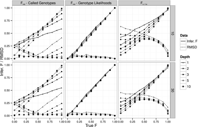
To assess the accuracy of our method, we applied it to a simulated data set of 10,000 variable sites under several different parameter combinations. For each of the 495 combinations of parameters, we estimated the inbreeding coefficients per site (Fsite) and plotted them together with their associated root mean square deviation (RMSD). Our results show that this method has reasonably good accuracy in estimating inbreeding coefficients per site with sequencing coverage >3×, sample sizes of 30 individuals, and an error rate of 0.5% (Fig. 1, right column). However, not surprisingly, high error rates, low coverage, and small sample sizes will result in reduced accuracy compared with estimates based on full knowledge of the genotypes (Supplemental Fig. 1). As typical for a bounded parameter, for small sample sizes the estimator becomes heavily biased when the true value is close to the boundary of the parameter space.
Figure 1.
Estimation of inbreeding coefficients. Performance of the EM method to infer Find from called genotypes (left column), Find from genotype likelihoods (center column), and Fsite (right column), for a sample size of 10 (first row) and 30 (second row) individuals and 10,000 variable sites simulated with a 0.5% error rate. Line styles and symbols represent different simulated sequencing coverages. Filled lines represent the inferred value for each simulated scenario (Infer. F), while dotted lines represent its RMSD.
Estimating individual inbreeding coefficients from simulated data
Although inbreeding coefficients per site can be useful for quality control (filtering sites that depart from HWE), a more interesting and biologically meaningful parameter is the inbreeding coefficient per individual. Estimates of this parameter can shed light into the species’ mating system and past history (domestication), as well as be used as a prior to improve genotype-calling algorithms. To this end, we extended a recently published algorithm by Hall et al. (2012) to estimate per-individual inbreeding coefficients directly from genotype likelihoods.
To assess the accuracy of this method, we applied it to the same simulated data set as in the previous section. For each of the 495 combination of parameters, we estimated inbreeding coefficients per individual (Find) and plotted them together with their associated RMSD. In all surveyed scenarios, the method presented here largely outperformed the original one, with lower RMSD and estimates closer to the true value (Fig. 1, left and center columns). This trend is even clearer in cases of extremely low coverage (1×), small sample sizes (10 individuals), and high error rates (Supplemental Figs. 2, 3). As an example, in a 1× data set with an average error rate of 0.5% and a sample size of 10 individuals, we obtain very accurate estimates, with the RMSD always smaller than 0.085, while the original method, applied to called genotypes, resulted in RMSDs as high as 0.41.
In these simulations, we assumed all sites to be independent. However, in real data, loci are linked, resulting in a lower number of available independent loci. In a partially selfing population, where S is the proportion of selfing, the effective population size is reduced by a factor of 1 − S/2 and the effective recombination rate is reduced by a factor of  (Golding and Strobeck 1980). As an example, with a selfing rate of S = 2/3, the effective recombination rate is reduced by a factor of 2, effectively reducing the number of independent loci. To assess the impact of a reduced number of effective sites on our estimates, we repeated the same simulations using half the effective number of independent variable sites (5000) and obtained similar results (Supplemental Fig. 4). Furthermore, and to fully address the impact of non-independence of sites, we simulated a more realistic 5-Mb genomic sequence, using as parameters previous estimates for rice populations and two realistic self-pollinating rates (S ∈ {0.7, 0.95}) (for details, see Methods). If all inbreeding is due to selfing, these rates correspond to theoretical inbreeding coefficient values of 0.54 and 0.90 (
 ) (Haldane 1924). Using our method, we obtained relatively accurate estimates of 0.64 and 0.84, respectively, demonstrating the robustness of the presented method even in the presence of linked sites. We notice that when sites are not independent the ML estimator is not truly a ML estimator and, therefore, should be considered a composite likelihood estimator. To form a proper ML inference procedure, data can be filtered to remove linked sites, but such filtering will lead to a loss of information.
This method turned out to be quite slow (on average 3.5 min and 147 iterations) and led us to develop a faster approximate algorithm that can be used for the initial iterations of the algorithm, greatly speeding up the analysis when analyzing large data sets (see Methods).
Effect of inbreeding on genotype calling
Several factors can bias genotype calling, including high error rates, inbreeding, sequencing coverage, and small sample sizes. To assess the impact of inbreeding on genotype call performance, we used the previously mentioned simulated data to call genotypes using a Bayesian approach under two different priors for the genotype frequencies: random mating (HWE; F = 0) and inferred inbreeding coefficient.
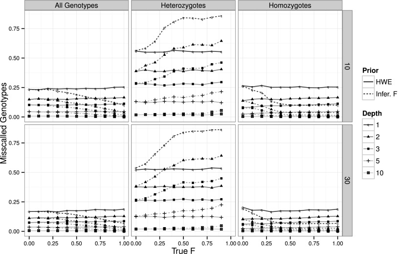
Assuming random mating in the prior yields constant genotype-calling error rates, independently of the sample inbreeding levels. When all sites are considered, proportions of miscalled genotypes are between 0.1 and 0.25, being unequally distributed between heterozygotes and homozygotes: 0.3–0.55 and 0.1–0.25, respectively (Fig. 2). However, in highly inbred samples, being able to incorporate inbreeding in the prior can greatly reduce genotype-calling errors, often to less than half of when assuming HWE (Fig. 2, left column). Considering homozygous and heterozygous genotypes separately provides additional insight into the effect of the priors. When assuming inbreeding, heterozygous genotype calling performs slightly worse (∼30%) since the prior assigns a lower probability on heterozygote genotypes (Fig. 2, center column). However, this increase in the heterozygous genotype-calling error rate is offset by the improvement in homozygous genotype calling, here assuming that inbreeding greatly reduces this error by as much as 60% (Fig. 2, right column). This level of improvement can be very important if we consider that highly inbred samples are almost exclusively homozygous (see also Supplemental Figs. 6–8).
Figure 2.
Effect of the inbreeding coefficient on genotype calling. Performance of genotype calling globally (left column), on just heterozygous genotypes (center column) and just homozygous genotypes (right column), on a sample size of 10 (first row) and 30 (second row) individuals and 10,000 variable sites simulated with a 0.5% error rate. Line styles and symbols represent different simulated sequencing coverages. Line types represent the level of inbreeding assumed in the priors: F = 0 (HWE; filled) and inferred value of F (Infer. F; large dashes). Missing F = 1 values reflect the absence of heterozygous genotypes on a totally inbred sample.
Effect of inbreeding on SFS
Allele frequencies and their distribution are important summaries of population genetic data analyses (Li 2011). Many widely used statistics such as Tajima’s D, Fu and Li’s D, Fay and Wu’s H, or FST (Nielsen 2005; Holsinger and Weir 2009) are direct functions of the SFS. These statistics can be used to infer demographic histories and to quantify the effect of natural selection. Given their importance in population genetic studies, it is of great interest to be able to estimate them reliably.
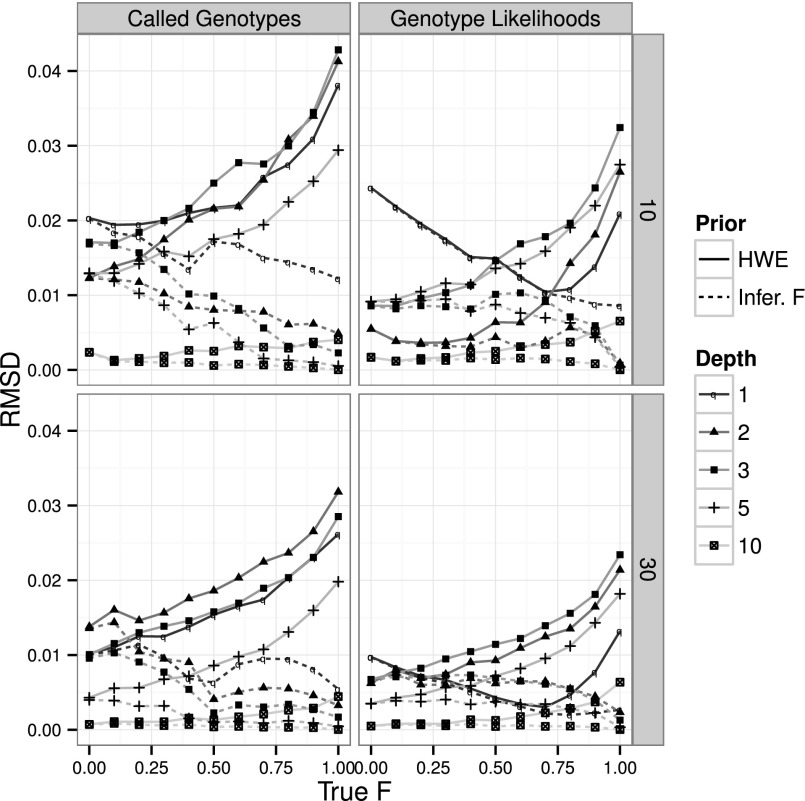
To assess the magnitude of inbreeding-related errors associated with SFS estimation, we inferred the SFS on the same simulated data set and under the same priors for the genotype frequencies as before: random mating (HWE; F = 0) and inferred inbreeding coefficient. We used both the standard approach based on called genotypes (see Methods) and a recent probabilistic method by Nielsen et al. (2012). High inbreeding coefficients have a marked effect on SFS estimation, and can increase the RMSD in the estimate of the SFS many fold (Fig. 3; Supplemental Figs. 9, 10). The inclusion of a correct prior will eliminate this problem, providing estimates of the SFS that are as good, or better, than the estimates obtained in the presence of no inbreeding. Not surprisingly, the probabilistic method performs overall better than using called genotypes. However, the difference between using called genotypes and the probabilistic approach is much smaller here than observed in other studies (Kim et al. 2011; Nielsen et al. 2012), because only true SNPs are included in these simulations, alleviating the problem of an excess of false singletons (and to a lesser degree doubletons) in methods based on genotype calling.
Figure 3.
Effect of the inbreeding coefficient on SFS estimation. Performance of SFS estimation from called genotypes (left column) and the Nielsen et al. (2012) method from GL and assuming inbreeding (right column), on a sample size of 10 (first row) and 30 (second row) individuals and 10,000 variable sites simulated with a 0.5% error rate. Line styles and symbols represent different simulated sequencing coverages. Line types depict the level of inbreeding assumed in the priors: F = 0 (HWE; filled) or inferred value of F (Infer. F; large dashes).
Application to real data
To illustrate the relevance of our method, we applied it to a publicly available data set of both wild and domesticated (cultivated) rice accessions (Xu et al. 2011). Cultivated rice (Oryza sativa) is classified into two major subspecies (O. s. japonica and O. s. indica) and further subdivided into genetically differentiated groups. There are also several species of wild rice, with the Oryza rufipogon species complex thought to be the closest to domesticated rice (e.g., Grillo et al. 2009; Wei et al. 2012). This species complex includes two forms: one perennial, photoperiod sensitive, and partially cross-fertilized (O. rufipogon); and another annual, photoperiod insensitive, and predominantly self-fertilized (Oryza nivara). The phenotypic differences between them have spurred a longstanding debate over the origins of cultivated rice, with some works assuming them to be different species (Sang and Ge 2007; Grillo et al. 2009), while others consider them as just ecotypes of a single species (Oka 1988; Zhu et al. 2007; Huang et al. 2012a; Wei et al. 2012).
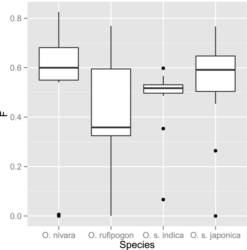
The diversity of mating systems, as well as the presence of both domesticated and wild forms, makes rice an interesting system for which to validate our newly developed methods. Among wild accessions the self-crossing rate is quite variable, although O. rufipogon tends to have lower rates than O. nivara: 50%–80% and 75%–95%, respectively (Morishima et al. 1984; Oka 1988; Gao et al. 2002; Phan et al. 2012). As for the cultivated accessions, they are thought to be almost totally inbred with self-crossing rates close to 95%, although O. s. indica has been described as having slightly lower rates (Oka 1988). Using our method, we aimed to estimate per-individual inbreeding coefficients of all studied 65 rice accessions. Since the level of population structure is not clear for these species, we analyzed each one of them separately. Our estimates show O. rufipogon with an intermediate level of inbreeding (Find ∼ 0.35), while Oryza nivara, O. s. indica, and O. s. japonica present significantly higher values around 0.6, 0.52, and 0.6, respectively (Fig. 4; Supplemental Table 1).
Figure 4.
Boxplot analysis of inferred per-individual inbreeding estimates. Each population was analyzed independently and the inferred inbreeding coefficients plotted.
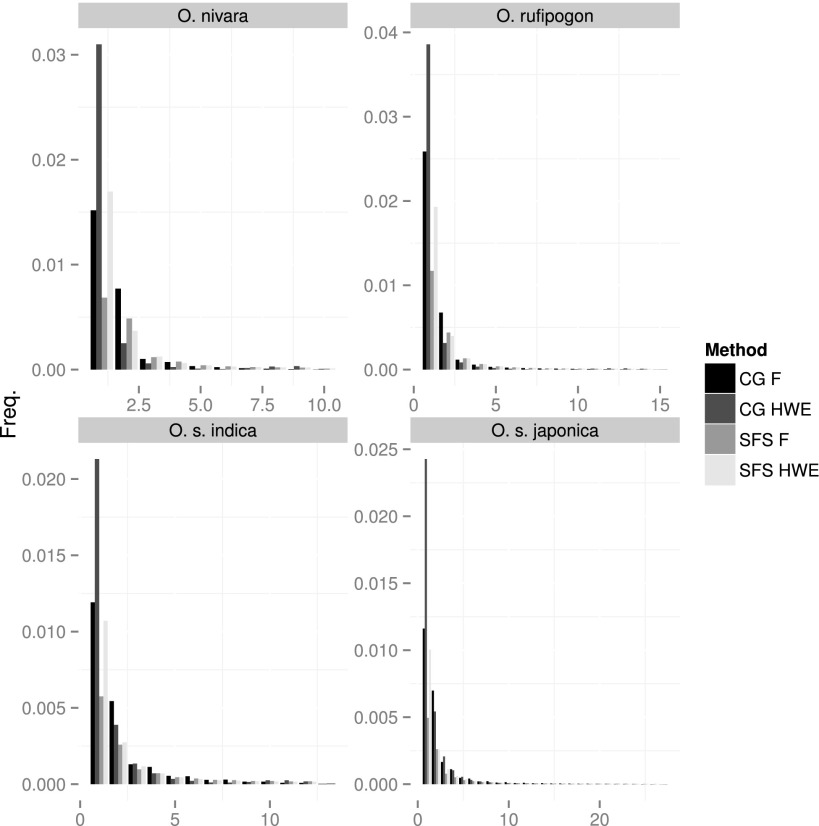
To assess the impact of explicitly assuming inbreeding on SFS estimation, we estimated it for each of the four rice species/subspecies. We used two different priors (random mating and estimated inbreeding coefficients) over two different methods (the probabilistic method by Nielsen et al. 2012 and using calling genotypes). Figure 5 shows that even for high coverage data (∼10×) (O. s. indica and O. s. japonica in Fig. 5), methods assuming HWE have an excess of singletons compared with methods that take inbreeding into account. This is a result of the greater weight the HWE prior gives to heterozygous genotypes, and the effect is stronger for genotype-calling methods than for the probabilistic method providing direct estimates of the SFS. In the data sets that also include low coverage samples (<5×) (Fig. 5, top row), the probabilistic method gives similar results irrespective of the prior used. However, the genotype-calling method, particularly assuming HWE, estimates many more singletons than other methods. However, both data sets contain high (10×) and low (2×–3×) coverage samples. To make sure the observed SFS differences were not caused by the presence of high-coverage accessions in the sample, we repeated the analysis on just the 10 low-coverage O. rufipogon accessions and found a similar trend (Supplemental Fig. 11). All in all, these results illustrate the importance of taking inbreeding into account when estimating allele frequencies, particularly in methods based on genotype calling.
Figure 5.
Estimated SFS on the analyzed rice population. SFS was estimated on the four populations using called genotypes (CG) and the Nielsen et al. (2012) method (SFS). In both cases, two priors were used: random mating (HWE) and inferred per-individual inbreeding estimates (F).
Discussion
While sequencing is becoming cheaper, there is an increasing demand for larger data sets, suggesting that low-coverage data will be common for years to come. When analyzing such data there can be considerable uncertainty, and inbreeding may, as illustrated by our results, have a marked effect on downstream analyses. Current NGS data analyses methods are mostly tuned for human populations and usually assume that the populations are in HWE. Although this is true for many species (e.g., human and mouse), there are self-pollinating plants (e.g., Arabidopsis) and domesticated species (e.g., rice, maize, dog), as well as species with asexual life cycles (e.g., daphnia, aphids, wasps) that are expected to have extremely high levels of inbreeding. Furthermore, many NGS data sets are being produced for domesticated species, due to their economic importance, and many of these species have significant amounts of inbreeding. It is therefore of great importance to include techniques for incorporating inbreeding when analyzing NGS data.
In this study, we developed algorithms to deal with inbred NGS data, either by estimating inbreeding coefficient per site or per individual. The per-site algorithm is mainly aimed at NGS quality control by removing sites that deviate from HWE. Usually, these deviations are done by comparing the expected genotype frequencies under HWE with the observed ones through a χ2 or Fisher’s exact test. However, in such analyses, genotypes need to be called first, possibly introducing biases in the downstream analyses. Our approach forms the basis for a likelihood ratio test for deviations from HWE (H0: F = 0) that can directly test the sites before calling genotypes.
Nevertheless, a more interesting and biologically meaningful parameter is the inbreeding coefficient per individual. This can shed light into the species’ mating system and past history (domestication), as well as be used as a prior in genotype calling, SFS, or other algorithms. Several methods have been published to infer per-individual inbreeding coefficients (Vogl et al. 2002; Leutenegger et al. 2003; Wang et al. 2006; Moltke et al. 2011), but all were designed for genotype (marker) data. Although all present slight improvements, Hall et al. (2012) recently incorporated most features into a single EM algorithm and showed that it outperformed previous methods. Here, we have modified this algorithm to accommodate for NGS data, as well as an approximate EM algorithm that can help speed up convergence. We notice that the rate of convergence can be further increased by using an accelerated EM approximation (Jamshidian and Jennrich 1993), although such an approach was not pursued here since we considered the running times to be acceptable (Supplemental Table 2).
In all scenarios examined, the new method presented here largely outperformed the original Hall et al. (2012) method based on called genotypes, especially in cases of extremely low coverage, small sample sizes, and high error rates. Because the original method has been previously shown to outperform other methods based directly on genotypes (Hall et al. 2012), the advantage of our method, in the presence of genotype uncertainty, should extend to these methods as well. Our analyses of simulated data further show that failing to use a correct prior can greatly affect downstream analyses. Genotype-calling errors can be more than twofold reduced by incorporating inbreeding into the genotype-calling algorithm, and there is an even more marked effect on the estimation of the SFS. Here, genotype-calling methods combined with erroneous assumptions of HWE when analyzing data from highly inbred species can lead to severe biases. Our real data analysis further supported these results.
We note that this manuscript distinguishes between inbreeding per site and per individual, with the main algorithm focusing on individual inbreeding coefficients and their application in genotype calling. The estimated inbreeding coefficient is a probability of identity by descent and is a property of an individual, implicitly assumed to be caused by cycles in the pedigree. As such, we do not attempt to assign particular individual segments as identical by descent (IBD) for genotype calling. Nevertheless, we note that the inference of individual IBD tracts, using hidden Markov model (HMM) style approaches, might improve both inferences regarding IBD and genotype calling. However, the implementations of such methods are computationally challenging, particularly because LD may strongly affect inferences regarding local IBD tracts (e.g., Moltke et al. 2011).
As a final remark, although our lower tested coverage was 1×, we expect our algorithm to perform equally well at ultra low coverages (e.g., 0.1× or 0.5×), given that enough variable sites with at least two sampled reads from the same individual are available (as a rule of thumb, at least around 1000).
Methods
Throughout this work we use the following notation:
n = number of individuals
k = number of loci
Xil = read data for individual i at locus l
Gil = genotype of individual i at locus l (member of Z)
Z = {AA, Aa, aa} or {0, 1, 2}
fl = allele frequency at locus l
fpq = frequency of genotype pq
Fi = inbreeding coefficient for individual i
Furthermore, vectors and matrices are depicted in bold (e.g., F or X), while scalars are not. Parameter estimates are depicted with a hat (e.g.,  ), while intermediate iteration EM estimates are depicted with a tilde (e.g.,
  ). When discussing methods for a single site, we drop the indicator for the identity of the site in the notation.
EM algorithm for per-site inbreeding estimation
For per-site inbreeding coefficients, the likelihood function, based on genotype likelihoods, is defined as
 |
where p(Xi|G) is the genotype likelihood and p(G|f, F) its prior (Eq. 2). An ML algorithm for maximizing this function is obtained by replacing the observed genotype counts in Equation 3 with the posterior expectation for genotype counts. To maximize the likelihood function, we use an EM algorithm to, iteratively, improve estimates of f and F. Using p(Gi = g|Xi) as a shorthand notation for  , the posterior probability of genotype g in individual i:
 |
 |
where E[HE] is calculated as in Equation 6 replacing  with
with  . The posterior at the jth step of the iteration can be calculated as
 |
A likelihood ratio can then be constructed by comparison of the likelihood function evaluated at the ML estimate of F and f to the likelihood assuming F = 0 to form a likelihood ratio test of the HWE.
EM algorithm for per-individual inbreeding estimation
There is little reason to assume that all individuals are equally inbred. On the contrary, when averaged over many individuals, we would expect the same inbreeding coefficient in each site if there has been no natural selection for or against inbreeding. In addition, inbreeding estimates based on individuals sites are likely to have large associated variances. For these reasons, priors for genotype calling are more conveniently based on inbreeding estimates that are allowed to vary among individuals, but not among sites. The following sections are devoted to describing such methods.
Assuming independence among sites, the expectation of the log likelihood under this model is obtained by replacing the indicator functions in Equation 7 with the posterior probability of the genotype. Using p(Gil = g|Xil) as a shorthand notation for p(Gil = g|Xil, fl, Fi):
 |
Hall et al. (2012) have recently proposed an EM algorithm to estimate per-individual inbreeding coefficients from genotype data. To maximize Equation 12, we extend their method for the use of genotype likelihoods (instead of known genotypes). Adapting Equation 11 from their paper to account for genotype uncertainty, for an individual i:
 |
where  is the posterior probability that the two alleles at locus l are identical by descent (IBD) at iteration j. This can be calculated using p(G|Xil), the genotype posterior probability, and
  as
as
 |
where  is the probability that two alleles at locus l are not IBD at iteration j. In the end, Equation 13 results in
 |
A similar extension to their update for allele frequencies  leads to
 |
As pointed out by Hall et al. (2012), the EM algorithm can converge to a local rather than a global maximum (Wu 1983), and, for this reason, several different starting values should be used. Additionally, rather than using random values as initial values, Equation 5 can be used to obtain initial estimates of Fi,  replacing observed genotype counts with their expected value.
Approximated EM for per-individual inbreeding estimation
The EM algorithm in Hall et al. (2012) is derived by treating the inbreeding status (inbred or not) in a single site as latent data. However, a faster algorithm can be derived by approximating an analytical solution to the maximization step for Fi in Equation 12. This method is not guaranteed to converge to the global maximum, but, since it initially converges considerably faster, it can be used in the initial iterations of the algorithm, greatly speeding up the previous method.
For a particular individual, to maximize values of Fi, we find the partial derivative of Equation 12 in order with Fi and set it equal to zero:
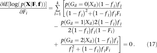 |
Since this expression cannot be solved numerically, we approximate it using an expansion around  (current value of Fi in an iterative algorithm) to obtain an approximate expression that can be optimized analytically. Equation 17 is composed of functions of F of the form [a/(b + Fc)], which can be expanded to
 |
Ignoring terms of order  and higher, Equation 17 can then be rewritten as
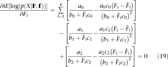 |
where
 |
 |
Solving for Fi (for  , fl ≠ 0):
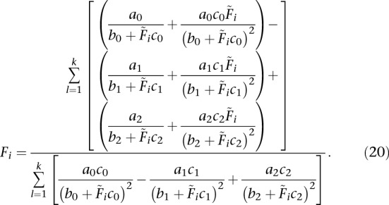 |
The algorithm then proceeds iteratively using Equation 19 with  and
and  . As the algorithm proceeds, the difference between
  and Fi decreases, providing a progressively more accurate approximation. However, as the joint update of F and f is not a joint maximization of the same expected log likelihood, it may lead the algorithm to be stuck in saddle point. To ensure eventual convergence, we then revert to our extension of the Hall et al. (2012) method for the last iterations of the algorithm.
Genotype calling
To call genotypes, we use a Bayesian approach to integrate over several error sources including base quality score and mapping quality score. We use the genotype likelihood at each site l and for each individual i (Eq. 1), together with a prior, to calculate the posterior probability of the genotypes and call the genotype with the highest probability (Li 2011; Nielsen et al. 2011, 2012). As a prior we use either the expected genotype frequencies under (1) HWE or (2) HWE assuming the estimated inbreeding coefficients, using the MAF calculated according to Kim et al. (2011).
Site frequency spectrum estimation
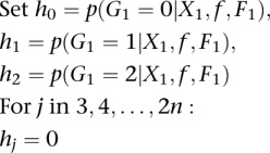
Estimation of the SFS can be achieved in several ways. Standard SFS estimation methods rely on first calling genotypes and then calculating allele frequencies at each position, but this approach is prone to bias and can greatly influence the results, especially at low coverage (Johnson and Slatkin 2008). Here, we consider an extended version of the SFS (since we also consider sites in the alignment that are fixed) that avoids the genotype-calling step. Instead, this method bases its inferences on the posterior probability (calculated with a prior accounting for HWE deviations) of the allele frequency for each site (Nielsen et al. 2012). Correcting a typo in the Nielsen et al. (2012) section “Incorporating Deviations from Hardy–Weinberg Equilibrium” and suppressing the site index in the notation, their algorithm should be
INITIALIZATION:
 |
RECURSION:
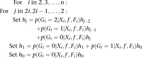 |
where p(Gi = g | Xi, f, Fi) is the posterior probability for individual i and genotype g, using the ML estimates of f and Fi. For a global estimate of the SFS, we sum each category (hj) across all sites and condition the SFS to only include variable sites:
 |
NGS data simulation
We performed extensive simulation studies to assess the performance of our methods and the effect of inbreeding on downstream analyses. Specifically, we assessed (1) the accuracy of the inbreeding coefficient estimates (both per site and per individual), (2) the impact of inbreeding on genotype calling, and (3) the influence of inbreeding in the estimation of the SFS. Due to computational constraints, we simulated mapped sequencing data rather than raw sequencing reads, similarly to previous studies (Kim et al. 2010, 2011). Each individual genotype was simulated assuming di-allelic loci with a given MAF for each locus and inbreeding coefficient F. In each locus, the number of reads was drawn from a Poisson distribution with the mean equal to the specified individual sequencing coverage. To simulate errors, each read base was changed to any of the other nucleotides at an equal rate ε/3, where ε is the error rate.
We simulated 10,000 variable sites on 10, 30, and 50 individuals, over average sequencing coverages of 1, 2, 3, 5, and 10×, with error rates of 0.5%, 1%, and 2%, and varied inbreeding coefficients from 0.0 to 1.0 in steps of 0.1, for a total of 495 combinations. With these parameter choices, we tried to focus on relatively extreme data sets (small sample sizes and low coverage), with realistic error rates (Glenn 2011) and covering biologically relevant scenarios of inbreeding from <0.07 in humans (Carothers et al. 2006) and ∼0.3 in dogs (Kirkness et al. 2003; Gray et al. 2009) to 0.4–0.98 in rice (Kovach et al. 2007) and 0.757 in wasps (Chapman and Stewart 1996).
We also simulated an extra data set, for validation purposes, of 1 million sites where only 1% are truly variable (true SNPs). We kept the same error rates, number of individuals, coverage, and inbreeding coefficients as before, for a total of 165 combinations of parameter values. Simulated data with only true SNPs, and with both true SNPs and invariable sites, yielded similar results (Supplemental Figs. 1–3, 5). For computational reasons, we therefore proceeded to use only the first data set in the rest of the analyses.
To test our method under linked loci, we performed a couple more simulation analyses. First, we simulated half the previous number of variable sites (5000), under the same 495 parameter combinations as before. Second, we simulated a 5-Mb genomic region across 30 accessions from one rice population, using the software SFS_CODE (Hernandez 2008). We assumed an effective population size of 125,000 (Caicedo et al. 2007; Asano et al. 2011), a mutation rate of 10−8 (Caicedo et al. 2007), a recombination rate of 4 cM/Mb (Tian et al. 2009; Asano et al. 2011), and two realistic self-pollinating rates of 0.7 and 0.95 (Oka 1988) (‘–theta 0.005 –rho 0.02 –self [0.7,0.95] –sampSize 30’). We then used the program ART (Huang et al. 2012b) to simulate 2× coverage 100-bp mapped reads with no indels directly in SAM format (‘–len 100 –fcov 2 -ir 0 -dr 0 -ir2 0 -dr2 0 -qs 10 -qs2 10 -sam’).
For the estimation of inbreeding coefficients (both from simulated and real data), we only use called SNPs with a log likelihood ratio (LRT) >15.1366 (χ2; P < 1 × 10⁻⁴; 1 d.f.), against the null hypothesis of f = 0, as implemented in the software ANGSD.
Error estimates
We calculated errors associated with the inbreeding coefficient estimates (F), genotype calling, and SFS estimation. For inbreeding estimates and SFS estimation, we used the RMSD. More specifically:
where Xtrue and Xest are the true and estimated values of the parameters, and S the total number of estimates. For estimates of Find, S is the total number of individuals, for Fsite the effective number of sites, and for the SFS the number of categories (S = 2n + 1). For genotype calling, the associated error was calculated as the proportion of miscalled genotypes. All plots were made using the R package ggplot2 (Wickham 2009).
Analysis of real data
In addition to simulated data, we also analyzed previously published Illumina GA II technology data from Rice, O. sativa (Xu et al. 2011). These data consist of 40 domesticated rice accessions, representative of all major Asian rice groups (27 O. s. japonica and 13 O. s. indica), together with five O. nivara and five O. rufipogon wild accessions at an effective (after mapping) sequencing coverage of 10×. The data set also includes an additional 15 wild rice accessions (10 O. rufipogon and five O. nivara) at an effective sequencing coverage of between 2× and 3×.
We used the originally mapped reads but performed de novo quality controls using only sites with minimum root mean square (RMS) mapping quality >10, maximum P-value for (strand bias, base quality bias, map quality bias, end distance bias, and HWE excess of heterozygous exact test) >10−4, and total coverage between 57× and 2645× for 65 individuals, but where at least half the individuals had at least 2× coverage (Minoche et al. 2011). After filtering, we calculated the genotype likelihoods with the SAMtools program (Li et al. 2009b) and used them in all subsequent analyses. Again, we only used variable sites for the estimation of inbreeding coefficients.
Software availability
The methods presented in this work were implemented in C/C++ and are freely available for non-commercial use. The per-site inbreeding coefficient’s (Fsite) estimation was incorporated into the software ANGSD, while the per-individual (Find) method was implemented in the stand-alone program ngsF. Both are available at http://cteg.berkeley.edu/∼nielsen/resources/software/ or, in the case of ngsF, also at https://github.com/fgvieira/ngsF.
Acknowledgments
We thank Thorfinn Korneliussen for helpful discussions and assistance in the use of ANGSD. Funding for this work was supported by an NIH grant to R.N., EMBO Long-Term Fellowship ALTF 2011-229 to M.F., and a Villum Foundation fellowship to A.A.
Footnotes
[Supplemental material is available for this article.]
Article published online before print. Article, supplemental material, and publication date are at http://www.genome.org/cgi/doi/10.1101/gr.157388.113.
References
- The 1000 Genomes Project Consortium 2010. A map of human genome variation from population-scale sequencing. Nature 467: 1061–1073 [DOI] [PMC free article] [PubMed] [Google Scholar]
- Asano K, Yamasaki M, Takuno S, Miura K, Katagiri S, Ito T, Doi K, Wu J, Ebana K, Matsumoto T, et al. 2011. Artificial selection for a green revolution gene during japonica rice domestication. Proc Natl Acad Sci 108: 11034–11039 [DOI] [PMC free article] [PubMed] [Google Scholar]
- Caicedo AL, Williamson SH, Hernandez RD, Boyko A, Fledel-Alon A, York TL, Polato NR, Olsen KM, Nielsen R, McCouch SR, et al. 2007. Genome-wide patterns of nucleotide polymorphism in domesticated rice. PLoS Genet 3: 1745–1756 [DOI] [PMC free article] [PubMed] [Google Scholar]
- Carothers AD, Rudan I, Kolcic I, Polasek O, Hayward C, Wright AF, Campbell H, Teague P, Hastie ND, Weber JL 2006. Estimating human inbreeding coefficients: Comparison of genealogical and marker heterozygosity approaches. Ann Hum Genet 70: 666–676 [DOI] [PubMed] [Google Scholar]
- Ceppellini R, Siniscalco M, Smith CA 1955. The estimation of gene frequencies in a random-mating population. Ann Hum Genet 20: 97–115 [DOI] [PubMed] [Google Scholar]
- Chapman TW, Stewart SC 1996. Extremely high levels of inbreeding in a natural population of the free-living wasp Ancistrocerus antilope (Hymenoptera: Vespidae: Eumeninae). Heredity 76: 65–69 [Google Scholar]
- DePristo MA, Banks E, Poplin R, Garimella KV, Maguire JR, Hartl C, Philippakis AA, del Angel G, Rivas MA, Hanna M, et al. 2011. A framework for variation discovery and genotyping using next-generation DNA sequencing data. Nat Genet 43: 491–498 [DOI] [PMC free article] [PubMed] [Google Scholar]
- Gao LZ, Schaal BA, Zhang CH, Jia JZ, Dong YS 2002. Assessment of population genetic structure in common wild rice Oryza rufipogon Griff. using microsatellite and allozyme markers. Theor Appl Genet 106: 173–180 [DOI] [PubMed] [Google Scholar]
- Glenn TC 2011. Field guide to next-generation DNA sequencers. Mol Ecol Resour 11: 759–769 [DOI] [PubMed] [Google Scholar]
- Golding GB, Strobeck C 1980. Linkage disequilibrium in a finite population that is partially selfing. Genetics 94: 777–789 [DOI] [PMC free article] [PubMed] [Google Scholar]
- Gray MM, Granka JM, Bustamante CD, Sutter NB, Boyko AR, Zhu L, Ostrander EA, Wayne RK 2009. Linkage disequilibrium and demographic history of wild and domestic canids. Genetics 181: 1493–1505 [DOI] [PMC free article] [PubMed] [Google Scholar]
- Grillo MA, Li C, Fowlkes AM, Briggeman TM, Zhou A, Schemske DW, Sang T 2009. Genetic architecture for the adaptive origin of annual wild rice, Oryza nivara. Evolution 63: 870–883 [DOI] [PubMed] [Google Scholar]
- Haldane JBS 1924. A mathematical theory of natural and artificial selection, Part–I. Trans Camb Philos Soc 23: 19–41 [Google Scholar]
- Hall N, Mercer L, Phillips D, Shaw J, Anderson AD 2012. Maximum likelihood estimation of individual inbreeding coefficients and null allele frequencies. Genet Res 94: 151–161 [DOI] [PubMed] [Google Scholar]
- Hernandez RD 2008. A flexible forward simulator for populations subject to selection and demography. Bioinformatics 24: 2786–2787 [DOI] [PMC free article] [PubMed] [Google Scholar]
- Holsinger KE, Weir BS 2009. Genetics in geographically structured populations: Defining, estimating and interpreting FST. Nat Rev Genet 10: 639–650 [DOI] [PMC free article] [PubMed] [Google Scholar]
- Huang P, Molina J, Flowers JM, Rubinstein S, Jackson SA, Purugganan MD, Schaal BA 2012a. Phylogeography of Asian wild rice, Oryza rufipogon: A genome-wide view. Mol Ecol 21: 4593–4604 [DOI] [PubMed] [Google Scholar]
- Huang W, Li L, Myers JR, Marth GT 2012b. ART: A next-generation sequencing read simulator. Bioinformatics 28: 593–594 [DOI] [PMC free article] [PubMed] [Google Scholar]
- Jamshidian M, Jennrich RI 1993. Conjugate gradient acceleration of the EM algorithm. J Am Stat Assoc 88: 221 [Google Scholar]
- Johnson PLF, Slatkin M 2008. Accounting for bias from sequencing error in population genetic estimates. Mol Biol Evol 25: 199–206 [DOI] [PubMed] [Google Scholar]
- Kim SY, Li Y, Guo Y, Li R, Holmkvist J, Hansen T, Pedersen O, Wang J, Nielsen R 2010. Design of association studies with pooled or un-pooled next-generation sequencing data. Genet Epidemiol 34: 479–491 [DOI] [PMC free article] [PubMed] [Google Scholar]
- Kim SY, Lohmueller KE, Albrechtsen A, Li Y, Korneliussen T, Tian G, Grarup N, Jiang T, Andersen G, Witte D, et al. 2011. Estimation of allele frequency and association mapping using next-generation sequencing data. BMC Bioinformatics 12: 231. [DOI] [PMC free article] [PubMed] [Google Scholar]
- Kirkness EF, Bafna V, Halpern AL, Levy S, Remington K, Rusch DB, Delcher AL, Pop M, Wang W, Fraser CM, et al. 2003. The dog genome: Survey sequencing and comparative analysis. Science 301: 1898–1903 [DOI] [PubMed] [Google Scholar]
- Kovach MJ, Sweeney MT, McCouch SR 2007. New insights into the history of rice domestication. Trends Genet 23: 578–587 [DOI] [PubMed] [Google Scholar]
- Leutenegger AL, Prum B, Génin E, Verny C, Lemainque A, Clerget-Darpoux F, Thompson EA 2003. Estimation of the inbreeding coefficient through use of genomic data. Am J Hum Genet 73: 516–523 [DOI] [PMC free article] [PubMed] [Google Scholar]
- Li H 2011. A statistical framework for SNP calling, mutation discovery, association mapping and population genetical parameter estimation from sequencing data. Bioinformatics 27: 2987–2993 [DOI] [PMC free article] [PubMed] [Google Scholar]
- Li H, Ruan J, Durbin R 2008. Mapping short DNA sequencing reads and calling variants using mapping quality scores. Genome Res 18: 1851–1858 [DOI] [PMC free article] [PubMed] [Google Scholar]
- Li H, Handsaker B, Wysoker A, Fennell T, Ruan J, Homer N, Marth G, Abecasis G, Durbin R 2009a. The Sequence Alignment/Map format and SAMtools. Bioinformatics 25: 2078–2079 [DOI] [PMC free article] [PubMed] [Google Scholar]
- Li R, Li Y, Fang X, Yang H, Wang J, Kristiansen K, Wang J 2009b. SNP detection for massively parallel whole-genome resequencing. Genome Res 19: 1124–1132 [DOI] [PMC free article] [PubMed] [Google Scholar]
- Li Y, Vinckenbosch N, Tian G, Huerta-Sanchez E, Jiang T, Jiang H, Albrechtsen A, Andersen G, Cao H, Korneliussen T, et al. 2010. Resequencing of 200 human exomes identifies an excess of low-frequency non-synonymous coding variants. Nat Genet 42: 969–972 [DOI] [PubMed] [Google Scholar]
- Liti G, Carter DM, Moses AM, Warringer J, Parts L, James SA, Davey RP, Roberts IN, Burt A, Koufopanou V, et al. 2009. Population genomics of domestic and wild yeasts. Nature 458: 337–341 [DOI] [PMC free article] [PubMed] [Google Scholar]
- Martin ER, Kinnamon DD, Schmidt MA, Powell EH, Zuchner S, Morris RW 2010. SeqEM: An adaptive genotype-calling approach for next-generation sequencing studies. Bioinformatics 26: 2803–2810 [DOI] [PMC free article] [PubMed] [Google Scholar]
- Minoche AE, Dohm JC, Himmelbauer H 2011. Evaluation of genomic high-throughput sequencing data generated on Illumina HiSeq and genome analyzer systems. Genome Biol 12: R112. [DOI] [PMC free article] [PubMed] [Google Scholar]
- Moltke I, Albrechtsen A, Hansen TVO, Nielsen FC, Nielsen R 2011. A method for detecting IBD regions simultaneously in multiple individuals—with applications to disease genetics. Genome Res 21: 1168–1180 [DOI] [PMC free article] [PubMed] [Google Scholar]
- Morishima H, Sano Y, Oka HI 1984. Differentiation of perennial and annual types due to habitat conditions in the wild rice Oryza perennis. Plant Syst Evol 144: 119–135 [Google Scholar]
- Nagalakshmi U, Wang Z, Waern K, Shou C, Raha D, Gerstein M, Snyder M 2008. The transcriptional landscape of the yeast genome defined by RNA sequencing. Science 320: 1344–1349 [DOI] [PMC free article] [PubMed] [Google Scholar]
- Ng SB, Buckingham KJ, Lee C, Bigham AW, Tabor HK, Dent KM, Huff CD, Shannon PT, Jabs EW, Nickerson DA, et al. 2010. Exome sequencing identifies the cause of a Mendelian disorder. Nat Genet 42: 30–35 [DOI] [PMC free article] [PubMed] [Google Scholar]
- Nielsen R 2005. Molecular signatures of natural selection. Annu Rev Genet 39: 197–218 [DOI] [PubMed] [Google Scholar]
- Nielsen R, Paul JS, Albrechtsen A, Song YS 2011. Genotype and SNP calling from next-generation sequencing data. Nat Rev Genet 12: 443–451 [DOI] [PMC free article] [PubMed] [Google Scholar]
- Nielsen R, Korneliussen T, Albrechtsen A, Li Y, Wang J 2012. SNP calling, genotype calling, and sample allele frequency estimation from new-generation sequencing data. PLoS ONE 7: e37558. [DOI] [PMC free article] [PubMed] [Google Scholar]
- Oka HI. 1988. Origin of cultivated rice. Elsevier Science/Japan Scientific Societies Press, Tokyo. [Google Scholar]
- Phan PDT, Kageyama H, Ishikawa R, Ishii T 2012. Estimation of the outcrossing rate for annual Asian wild rice under field conditions. Breed Sci 62: 256–262 [DOI] [PMC free article] [PubMed] [Google Scholar]
- Sang T, Ge S 2007. Genetics and phylogenetics of rice domestication. Curr Opin Genet Dev 17: 533–538 [DOI] [PubMed] [Google Scholar]
- Smith CAB, Thomson R 1988. Estimation of inbreeding from population samples. J Appl Probab 25: 127–135 [Google Scholar]
- Tian Z, Rizzon C, Du J, Zhu L, Bennetzen JL, Jackson SA, Gaut BS, Ma J 2009. Do genetic recombination and gene density shape the pattern of DNA elimination in rice long terminal repeat retrotransposons? Genome Res 19: 2221–2230 [DOI] [PMC free article] [PubMed] [Google Scholar]
- Vogl C, Karhu A, Moran G, Savolainen O 2002. High resolution analysis of mating systems: Inbreeding in natural populations of Pinus radiata. J Evol Biol 15: 433–439 [Google Scholar]
- Wang H, Lin CH, Service S, Chen Y, Freimer N, Sabatti C 2006. Linkage disequilibrium and haplotype homozygosity in population samples genotyped at a high marker density. Hum Hered 62: 175–189 [DOI] [PubMed] [Google Scholar]
- Wei X, Qiao WH, Chen YT, Wang RS, Cao LR, Zhang WX, Yuan NN, Li ZC, Zeng HL, Yang QW 2012. Domestication and geographic origin of Oryza sativa in China: Insights from multilocus analysis of nucleotide variation of O. sativa and O. rufipogon. Mol Ecol 21: 5073–5087 [DOI] [PubMed] [Google Scholar]
- Wickham H. 2009. Ggplot2: Elegant graphics for data analysis. Springer, New York. [Google Scholar]
- Wu CFJ 1983. On the convergence properties of the EM algorithm. Ann Stat 11: 95–103 [Google Scholar]
- Xia Q, Guo Y, Zhang Z, Li D, Xuan Z, Li Z, Dai F, Li Y, Cheng D, Li R, et al. 2009. Complete resequencing of 40 genomes reveals domestication events and genes in silkworm (Bombyx). Science 326: 433–436 [DOI] [PMC free article] [PubMed] [Google Scholar]
- Xu X, Liu X, Ge S, Jensen JD, Hu F, Li X, Dong Y, Gutenkunst RN, Fang L, Huang L, et al. 2011. Resequencing 50 accessions of cultivated and wild rice yields markers for identifying agronomically important genes. Nat Biotechnol 30: 105–111 [DOI] [PubMed] [Google Scholar]
- Zhu Q, Zheng X, Luo J, Gaut BS, Ge S 2007. Multilocus analysis of nucleotide variation of Oryza sativa and its wild relatives: Severe bottleneck during domestication of rice. Mol Biol Evol 24: 875–888 [DOI] [PubMed] [Google Scholar]


