A Cut Cell Method for Simulating Spatial Models of Biochemical Reaction Networks in Arbitrary Geometries

Abstract

Cells use signaling networks consisting of multiple interacting proteins to respond to changes in their environment. In many situations, such as chemotaxis, spatial and temporal information must be transmitted through the network. Recent computational studies have emphasized the importance of cellular geometry in signal transduction, but have been limited in their ability to accurately represent complex cell morphologies. We present a finite volume method that addresses this problem. Our method uses Cartesian cut cells and is second order in space and time. We use our method to simulate several models of signaling systems in realistic cell morphologies obtained from live cell images and examine the effects of geometry on signal transduction.

1 Introduction

Cells must be able to sense and respond to external environmental cues. Information about external signals, such as hormones or growth factors, is transmitted by signaling pathways to the cellular machinery required to generate the appropriate response. Defects in these pathways can lead to diseases, such as cancer, diabetes, and heart disease. Therefore, understanding how intracellular signaling pathways function is not only a fundamental problem in cell biology, but also important for developing therapeutic strategies for treating disease.

In many pathways, proper signal transduction requires that both the spatial and temporal dynamics of the system are tightly regulated [1]. For example, recent experiments have revealed spatial gradients of protein activation in migrating cells [2]. Mathematical models can be used to elucidate the control mechanisms used to regulate the spatiotemporal dynamics of signaling pathways, and recent computational studies emphasize the importance of cellular geometry in signaling networks [3,4]. For computational simplicity, many of these investigations assume idealized cell geometries [4,5], whereas others approximate irregularly shaped cells using a “staircase” representation of the cell membrane [6]. Both finite element and finite volume methods have been used to simulate spatial models of biochemical reaction networks [4,7]. For finite element methods, which typically require a triangulation of the computational domain, grid generation can be a challenge. This becomes especially true if the boundaries of the computational domain are moving. To overcome this issue, we developed a finite volume method that utilizes a Cartesian grid. Our numerical scheme is based on a cut cell method that accurately represents the cell boundary using a piecewise-linear approximation. This approach allows us to achieve second order accuracy in space and time. Our method also provides an appropriate framework for addressing moving boundary problems using level set methods [8,9].

2 Mathematical Formulation

Spatial models of biochemical reaction networks are typically represented using partial differential equations consisting of reaction and diffusion terms. For simplicity we restrict ourselves to two spatial dimensions x and y. For a given chemical species, the reaction terms encompass processes such as activation, degradation, protein modifications and the formation of molecular complexes. These reactions typically include nonlinear terms, such as those arising from Michaelis-Menten kinetics. In a system consisting of n chemical species, the concentration of the i^th species c_i evolves in space and time according to the following equation:

$$\frac{\partial c_i}{\partial t}=-\nabla ·\mathbf{J}+f_i(\mathit{c}).$$ (1)

where J = −D_i∇c_i is the flux density, D_i is the diffusion coefficient, and the function f_i(c) models the reactions within the cell that affect c_i. The elements of the vector c are the concentrations of the n chemical species. Reactions also may occur on the cell membrane yielding mixed-type, nonlinear conditions on the boundary ∂Ω,

$$-D\overrightarrow{n}·{\nabla c_i|}_{\partial \mathrm{\Omega }}+{g(\mathit{c})|}_{\partial \mathrm{\Omega }}=0.$$ (2)

Eqs. (1) and (2) are solved subject to appropriate initial conditions c_i(x, y, 0) for each species in the system.

3 Numerical Methods

Our goal is to develop a simulation tool that can accurately and efficiently solve spatial models of signaling and regulatory pathways in realistic cellular geometries. We obtain the computational domain from live-cell images. The model equations are solved on a Cartesian grid by discretizing the Laplacian operator, which models molecular diffusion, using a finite volume method.

3.1 Computational domain

Fig. 1 shows a grayscale image of a mouse fibroblast [2]. Because the original image is noisy, the image was smoothed by convolving it twice with the standard five point Gaussian smoothing filter. After smoothing, a suitable thresholding value was picked, and the front was computed by an iso-contour finder. A signed distance function is constructed with the smoothened boundary using Fast Marching Methods [10]. The zero level set of the signed distance function yields piecewise linear segments used to define cut cells (Fig. 2).

Fig. 1.

Grayscale image of a mouse fibroblast taken from supplemental data in [2] (left) and the smoothened boundary (right).

Fig. 2.

Computational boundary (dashed line) with an assumed higher order representation of the cell boundary drawn as a solid line.

3.2 Discretization of the Spatial Operator

We utilize a Cartesian grid-based, finite volume algorithm originally presented in [11] to discretize the diffusion operator arising from Eq. (1). Finite volume methods store the average value of the concentration over a computational grid cell at the location (i, j). That is,

$${\mathrm{c̄}}_{i,j}=\frac{1}{V_{i,j}}\int {\int }_{V_{i,j}}c(x,y)dV,$$ (3)

where V_i,j is the volume of the (i, j) grid cell. Inserting Eq. (3) into Eq. (1) produces

$$\frac{\partial {\mathrm{c̄}}_{i,j}}{\partial t}-{\overline{f(c)}}_{i,j}=-\frac{1}{V_{i,j}}\int {\int }_{V_{i,j}}\nabla ·\mathbf{J}dV.$$ (4)

The divergence theorem allows us to convert the above volume integral into a surface integral,

$$\frac{\partial {\mathrm{c̄}}_{i,j}}{\partial t}-{\overline{f(c)}}_{i,j}=-\frac{1}{V_{i,j}}{\int }_{\partial V_{i,j}}(\mathbf{J}·\overrightarrow{n})dS.$$ (5)

For interior grid cells, we have

$$\frac{\partial {\mathrm{c̄}}_{i,j}}{\partial t}-{\overline{f(c)}}_{i,j}=-\frac{1}{V_{i,j}}\left[{\int }_{y_{j-1/2}}^{y_{j+1/2}}\right(J_x(x_{i+1/2},y)-J_x(x_{i-1/2},y))dy+{\int }_{x_{i-1/2}}^{x_{i+1/2}}(J_y(x,y_{j+1/2})-J_y(x,y_{j-1/2})\left)dx\right],$$ (6)

where $J_x=-D\frac{\partial c}{\partial x}$ and $J_y=-D\frac{\partial c}{\partial y}$. Approximation of the integrals in Eq. (6) with the midpoint rule yields

$$\frac{\partial c_{i,j}}{\partial t}-f(c_{i,j})\approx -\frac{1}{V_{i,j}}\left[\mathrm{\Delta }y\right(J_x(x_{i+1/2},y_j)-J_x(x_{i-1/2},y_j))+\mathrm{\Delta }x(J_y(x_i,y_{j+1/2})-J_y(x_i,y_{j-1/2})\left)\right].$$ (7)

By approximating the gradient terms with centered differences, we arrive at the standard five point Laplacian.

The cut cell method generalizes as follows. The boundary of the computational domain is approximated as a piecewise linear segments (Fig. 2, dashed line), and grid cells that the boundary passes through are referred to as cut cells. The volume of a cut cell is computed by recasting the volume integral as a boundary integral:

$$V_{i,j}=\int {\int }_{V_{i,j}}dV=\int {\int }_{V_{i,j}}\nabla ·{[\frac{x}{2},\frac{y}{2}]}^{T}dV={\int }_{\partial V_{i,j}}\left(\right[\frac{x}{2},\frac{y}{2}\left]\overrightarrow{n}\right)dS,$$ (8)

where the integral on the right can be computed exactly for the polygon. Each segment is evaluated, then summed. The center of mass can also be computed using a boundary integral, for example:

$$\int {\int }_{V_{ij}}xdV=\int {\int }_{V_{ij}}\nabla ·{[\frac{x^2}{2},0]}^{T}dV={\int }_{\partial V_{i,j}}\left(\right[\frac{x^2}{2},0\left]\overrightarrow{n}\right)dS.$$ (9)

Next, we construct the integral on the right side of Eq. (5) for a cut cell. In general, there are up to five surface integrals to approximate. Let a_l,m ∈ [0, 1] represent the portion of each of the four cell edges covered by the cut cell and a_f be the length of the line segment representing the boundary. Then Eq. (7) becomes

$$\frac{\partial c_{i,j}}{\partial t}-f(c_{i,j})\approx -\frac{1}{V_{i,j}}\left[\mathrm{\Delta }y\right(a_{i+1/2,j}{J}_x(x_{i+1/2},j)-a_{i-1/2,j}{J}_x(x_{i-1/2},y_j))+\mathrm{\Delta }x(a_{i,j+1/2}{J}_y(x_i,y_{j+1/2})-a_{i,j-1/2}{J}_y(x_i,y_{j-1/2}))+a^f{J}_f].$$ (10)

Let F_i±1/2,j = −a_i±1/2,jΔyJ_x(x_i±1/2, y_j) and F_i,j±1/2 = −a_i,j±1/2ΔxJ_y(x_i, y_j±1/2). With this notation, we rewrite the previous equation as

$$\frac{\partial c_{i,j}}{\partial t}-f(c_{i,j})\approx \frac{1}{V_{i,j}}(F_{i+1/2,j}-F_{i-1/2,j}+F_{i,j+1/2}-F_{i,j-1/2}-F_{i,j}^f).$$ (11)

We refer to the F’s as the surface fluxes (Fig. 3). On a full edge with a_l,m = 1 the surface flux is calculated with centered differences. For example, in Fig. 3, we have

$$F_{i+1/2,j}=D\mathrm{\Delta }y\frac{c_{i+1,j}-c_{i,j}}{\mathrm{\Delta }x}.$$ (12)

Fig. 3.

Diagram of fluxes for cut cells where shaded boxes indicate cells that are inside the boundary.

The flux gradient across a cut edge, e.g. (x_i−1/2, y_j), is approximated by a linear interpolation of two gradients, which are computed by centered differences. A linear interpolation formula between two points y₁ and y₂ as a function of a parameter μ ∈ [0, 1] is

$$y^I=(1-\mu )y_1+\mu y_2.$$ (13)

In the case of a cut cell edge, μ = (1 + a_l,m)/2. For example, to construct F_i−1/2,j in Fig. 3, the gradient at (x_i−1/2, y_j) and (x_i−1/2, y_j−1) is used,

$$F_{i-1/2,j}=D{a}_{i-1/2,j}\mathrm{\Delta }y[\frac{(1+a_{i-1/2,j})}{2}\frac{(c_{i-1,j}-c_{i,j})}{\mathrm{\Delta }x}+\frac{(1-a_{i-1/2,j})}{2}\frac{(c_{i-1,j-1}-c_{i-1,j-1})}{\mathrm{\Delta }x}].$$ (14)

To calculate the flux through a boundary, e.g. $F_{i,j}^f$, we compute the gradient along a line normal to the boundary and centered at the boundary midpoint. To find function values on the normal line, we interpolate using three equally spaced cell centered points (Fig. 4). If the normal line is oriented with an angle of π/4 < |θ| < 3π/4 relative to the horizontal grid lines, horizontal grid points are used to compute the values on the line. Otherwise vertical points are used. The two points computed along the normal line and the value on the boundary are then used to construct a quadratic polynomial. The concentration gradient is calculated by differentiating the quadratic polynomial and evaluating the result at the boundary point c_f,

$$G^f=\frac{1}{d_2-d_1}[\frac{d_2}{d_1}(c^f-c_1^I)-\frac{d_1}{d_2}(c^f-c_2^I)],$$ (15)

where $c_1^I$ and $c_2^I$ are the interpolated values along the normal line and d₁ and d₂, respectively, are the distances of these two points from the boundary. The flux $F_{ij}^f$ in Eq. (11) is calculated by multiplying G^f by the area of the cut-cell edge a_f and the diffusion coefficient D. Then the boundary condition Eq. (2) becomes the algebraic equation

$$D{G}^f+g({\mathit{c}}^f)=0.$$ (16)

Fig. 4.

Circles indicate interpolated values that depend on the square grid values.

Because all gradients are constructed with second order methods, the overall discretization scheme is second order in space. Further discussion on the accuracy of the spatial discretization scheme can be found in [11].

3.3 Time Discretization

Because of the boundary conditions in Eq. (2), operator splitting methods are limited to first order accuracy. Therefore we treat Eqs. (1) and (2) as a differential-algebraic system of non-linear equations. The general form of differential-algebraic system is

$$F(t,\mathit{C},\mathit{C}\prime )=0,$$ (17)

where C is a 2n × 1 vector. The first n entries in the differential-algebraic system of equations are formed by the discretization of Eq. (1) for the chemical species concentrations, and the (n+1)^th to 2n^th entries arise from the boundary conditions given in Eq. (2).

This formulation in conjunction with the discretization of the spatial operator presented in the previous sections allows us to use the DASPK solver described in [12]. Backward differentiation formulas are used to solve Eq. (17) with methods up to fifth order accurate in time. The resulting nonlinear system of equations is solved with a modified Newton’s method, given by

$${\mathit{C}}^{m+1}={\mathit{C}}^m-\gamma {(\alpha \frac{\partial F}{\partial \mathit{C}\prime }+\frac{\partial F}{\partial \mathit{C}})}^{-1}F(t,{\mathit{C}}^m,\alpha {\mathit{C}}^m+\beta ),$$ (18)

where α is a constant that changes when the order or step size changes, β is a vector that depends on the solution at previous time values, and γ is a constant chosen to speed up convergence. Note that each step of the Newton iteration requires inverting the matrix

$$A=\alpha \frac{\partial F}{\partial \mathit{C}\prime }+\frac{\partial F}{\partial \mathit{C}}.$$ (19)

We store this matrix in sparse triple format, and use routines from SPARSKIT [13] to solve the linear system iteratively. The Generalized Minimal Residual (GMRES) method [14] with an incomplete LU (ILU) preconditioner is used to solve the linear system. The combination of the second order accurate cut cell discretization of the Laplacian operator with the fifth order accurate DASPK time integrator yields an overall second order method with no splitting error.

4 Results

4.1 Convergence Tests

To demonstrate the accuracy of our method on a domain containing all types of cut cells, the convergence of our method is compared against an exact solution on a circle. The exact solution to the diffusion equation with a zero Dirichlet boundary condition can be found in terms of Bessel functions. Let λ denote the first root of the Bessel function J₀(x), and r be the radius of the circle. Then the expression:

$$f(x,y,t)=\text{exp}[-D{\left(\frac{\lambda }{r}\right)}^{2}t]J_0\left(\lambda \frac{\sqrt{{(x-0.5)}^2+{(y-0.5)}^2}}{r}\right)$$ (20)

is an exact solution to the diffusion equation. Fig. 5 shows the initial condition and the computed solution at t = 0.2 using the constants D = 0.05 and r = 0.3. For visualization purposes, the computational domain and boundary points are triangulated using Triangle [15]. The error in the infinity norm over time is shown in Fig. 6. These results demonstrate the second order accuracy of the numerical method.

Fig. 5.

Initial condition for the diffusion equation (left) and computed solution at t = 0.2 (right).

Fig. 6.

Error in the infinity norm for the diffusion equation.

Next we tested a nonlinear system in which a protein C can exist in two distinct chemical states: active and inactive. The reactions that convert the protein between the two states are assumed to follow Michaelis-Menten kinetics, which describes the kinetics of many enzymatic reactions including phosphorylation and dephosphorylation events [16]. The protein C is deactivated in the interior of the computational domain according to the following equations:

$$\frac{\partial C_i}{\partial t}=D\mathrm{\Delta }{C}_i+\frac{k_2{C}_a}{K_{m2}+C_a}\frac{\partial C_a}{\partial t}=D\mathrm{\Delta }{C}_a-\frac{k_2{C}_a}{k_{m2}+C_a}$$ (21)

where C_i and C_a are the concentrations of inactive and active protein, respectively, k₂ is the maximum deactivation rate, and K_m2 is the Michaelis constant. Activation occurs on the boundary, ∂Ω, according to the following boundary conditions:

$$-D\overrightarrow{n}·{\nabla C_i|}_{\partial \mathrm{\Omega }}=\frac{k_{1}S{C}_i}{K_{m1}+C_i}-D\overrightarrow{n}·{\nabla C_a|}_{\partial \mathrm{\Omega }}=-\frac{k_{1}S{C}_i}{K_{m1}+C_i}$$ (22)

where k₁ is the maximum activation rate and K_m1 is the Michaelis constant. The equations are solved in the domain

$$(r,\theta )=r\le 0.3-0.09\text{sin}(4\theta ).$$ (23)

The initial concentration of inactive protein is assumed to be constant and equal to 1. There is initially no active protein. Fig. 7 shows a plot of the concentrations at t = 0.25.

Fig. 7.

Concentrations of inactive (left) and active (right) species at t=0.25 with the coefficients D = 0.1, k₁ = k₂ = S = 1.0, and K_m1 = K_m2 = 0.2.

We compute the error as the difference between successive refinements of the grid. That is, E(x, y, t) = c_Δx(x, y, t) − c_Δx/2(x, y, t). Since the grids do not align, the values on the finer grid are averaged before subtracting the value on the courser grid. E(x, y, t) is defined on interior values of the course grid. By computing the error with this method, Fig. 8 shows second order convergence in the infinity norm for the chemical species C_i. The convergence plot of C_a was identical. The time step was set to Δx/4.

Fig. 8.

C_i error in the infinity norm

4.2 A two compartment model

In this model, we have two compartments: the cytoplasm and nucleus. The cellular geometry was taken from a yeast cell undergoing chemotrophic growth in the direction of a pheromone gradient [17]. The nucleus is modeled as a circle located toward the front of the cell. The model consists of two species, A and C, with inactive and active forms. Protein C is allowed to enter and exit the nucleus, whereas protein A is restricted to the cytoplasm. Initially both A and C are in their inactive forms. At t = 0, the reaction that activates A is initiated. This is meant to model the cell receiving an external signal. Once A is activated it is assumed to interact with the cell membrane, causing a reduction in the protein’s diffusion coefficient. Active A can then activate C. The active form of C is only deactivated within the nucleus. This simple model captures some of the signaling events that occur during the pheromone response of yeast. If we denote the concentration of a chemical species with brackets, the equations for the cytoplasmic species are:

$$\frac{\partial [A_c]}{\partial t}=D_1\mathrm{\Delta }[A_c]-k_0[A_c]\frac{\partial [A_c^{*}]}{\partial t}=D_2\mathrm{\Delta }[A_c^{*}]+k_0[A_c]\frac{\partial [C_c]}{\partial t}=D_1\mathrm{\Delta }[C_c]-k_1[A_c^{*}][C_c]\frac{\partial [C_c^{*}]}{\partial t}=D_1\mathrm{\Delta }[C_c^{*}]+k_1[A_c^{*}][C_c].$$

where the asterisks denote the active form of the protein, D₁ is the diffusion coefficient in the cytoplasm, D₂ is diffusion coefficient in the membrane, and the k’s represent the reaction rates. Subscripts indicate cytosolic and nuclear species. The boundary conditions at the cell membrane are no flux for all chemical species. The nuclear boundary conditions for A species are also no flux, whereas C species are allowed to move through the nuclear membrane and satisfy the conditions

$$-D_1{(\overrightarrow{n}·\nabla [C_c])|}_{\partial {\mathrm{\Omega }}_2}=-k_2{([C_n]-[C_c])|}_{\partial {\mathrm{\Omega }}_2}-D_1{(\overrightarrow{n}·\nabla [C_c^{*}])|}_{\partial {\mathrm{\Omega }}_2}=-k_2{([C_n^{*}]-[C_c^{*}])|}_{\partial {\mathrm{\Omega }}_2}-D_1{(\overrightarrow{n}·\nabla [C_n])|}_{\partial {\mathrm{\Omega }}_2}=k_2{([C_n]-[C_c])|}_{\partial {\mathrm{\Omega }}_2}-D_1{(\overrightarrow{n}·\nabla [C_n^{*}]|}_{\partial {\mathrm{\Omega }}_2}=k_2{([C_n^{*}]-[C_c^{*}])|}_{\partial {\mathrm{\Omega }}_2},$$

Nuclear C* is deactivated according to the equations

$$\frac{\partial [C_n]}{\partial t}=D_1\mathrm{\Delta }[C_n]+k_3[C_n^{*}]\frac{\partial [C_n^{*}]}{\partial t}=D_1\mathrm{\Delta }[C_n^{*}]-k_3[C_n^{*}].$$

Simulation results are shown in Figs. 9 and 10. All reaction constants were set to one, D₁ = 0.1, D₂ = 0.01, and Δx = 1/100. The initial values were zero except for [A_c] (x, y, 0) = [C_c] (x, y, 0) = 1. The system reached steady state at t = 10. The execution time of the simulation was 22 seconds on Mac Pro desktop computer with dual-core 2.66 GHz Intel Xeon processors. The model simulation suggests a spatial activation gradient can be generated by the position of the nucleus. The inactivation of C in the nucleus leads to a higher concentration of active protein in the rear of the cell in spite of a uniform spatial signal from active A.

Fig. 9.

Steady state concentration of inactive C in the cytoplasm and nucleus.

Fig. 10.

Steady state concentration values for inactive C species (left) and active C species (right).

4.3 Rho family GTPase Model

The Rho family of GTPases regulates many cellular functions, including polarization and motility. We created a model with three key members of this family, Cdc42, Rac, and Rho (Fig. 11). In our model, an extracellular signal triggers the activation of Cdc42 protein on the cell membrane,

$$-D\overrightarrow{n}·\nabla {[Cdc{42}_i]|}_{\partial \mathrm{\Omega }}=\frac{k_{1}S[Cdc{42}_i]}{K_{m1}+[Cdc{42}_i]}-D\overrightarrow{n}·\nabla {[Cdc{42}_a]|}_{\partial \mathrm{\Omega }}=-\frac{k_{1}S[Cdc{42}_i]}{k_{m2}+[Cdc{42}_i]}.$$ (24)

Fig. 11.

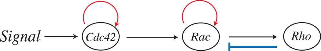
Schematic of Interactions

In the cell interior, active Cdc42 is inactivated. A positive feedback loop increases the activation of Cdc42,

$$\frac{\partial [Cdc{42}_i]}{\partial t}=D\mathrm{\Delta }[Cdc{42}_i]+\frac{k_2[Cdc{42}_a]}{K_{m3}+[Cdc{42}_a]}-\frac{k_3[Cdc{42}_a][Cdc{42}_i]}{K_{m4}+[Cdc{42}_i]}\frac{[\partial Cdc{42}_a]}{\partial t}=D\mathrm{\Delta }[Cdc{42}_a]-\frac{k_2[Cdc{42}_a]}{k_{m5}+[Cdc{42}_a]}+\frac{k_3[Cdc{42}_a][Cdc{42}_i]}{k_{m6}+[Cdc{42}_i]}.$$ (25)

Rac is activated by Cdc42, and a positive feedback loop increases the concentration of active Rac. Active Rho increases the deactivation of Rac in the cytosol,

$$\frac{\partial [Ra{c}_i]}{\partial t}=D\mathrm{\Delta }[Ra{c}_i]+\frac{(k_4[Rh{o}_a]+k_5)[Ra{c}_a]}{K_{m7}+[Ra{c}_a]}-\frac{(k_6[Cdc{42}_a]+k_7[Ra{c}_a])[Ra{c}_i]}{K_{m8}+[Ra{c}_i]}\frac{\partial [Ra{c}_a]}{\partial t}=D\mathrm{\Delta }[Ra{c}_a]-\frac{(k_4[Rh{o}_a]+k_5)[Ra{c}_a]}{k_{m9}+[Ra{c}_a]}+\frac{(k_6[Cdc{42}_a]+k_7[Ra{c}_a])[Ra{c}_i]}{k_{m10}+[Ra{c}_i]}$$ (26)

Rho is activated by the active form of Rac and deactivated in the interior,

$$\frac{\partial [Rh{o}_i]}{\partial t}=D\mathrm{\Delta }[Rh{o}_i]+\frac{k_8[Rh{o}_a]}{K_{m11}+[Rh{o}_a]}-\frac{k_9[Ra{c}_a][Rh{o}_i]}{K_{m12}+[Rh{o}_i]}\frac{\partial [Rh{o}_a]}{\partial t}=D\mathrm{\Delta }[Rh{o}_a]-\frac{k_8[Rh{o}_a]}{k_{m13}+[Rh{o}_a]}+\frac{k_9[Ra{c}_a][Rh{o}_i]}{k_{m14}+[Rh{o}_i]}$$ (27)

The boundary conditions for Rac and Rho species are no flux. The steady state distribution at t = 2.0 is displayed in Fig. 12. To achieve these results a step size Δx = 1/100 and a diffusion coefficient D = 0.1 were used. The reaction constants from the simulation are listed in Table 1. The initial concentration of inactive chemical species was set to one and zero for active species. The execution time was 39 seconds on a Mac Pro desktop computer with dual-core 2.66 GHz Intel Xeon processors.

Fig. 12.

Steady state distribution of protein concentration amounts in a fibroblast. The boundary was taken from a live cell image [2].

Table 1.

Reaction constants used in simulation of the Rho GTPase model.

S = 1	k4 = 3	k8 = 3	Km3 = 0.2	Km7 = 0.2	Km11 = 0.2
k1 = 5	k5 = 1	k9 = 5	Km4 = 0.2	Km8 = 0.2	Km12 = 0.2
k2 = 3	k6 = 5	Km1 = 0.2	km5 = 0.2	km9 = 0.2	km13 = 0.2
k3 = 1	k7 = 1	km2 = 0.2	km6 = 0.2	km10 = 0.2	k14 = 0.2

In this model, a gradient is formed by protein activation on the membrane. The gradient is propagated to the downstream signaling components Rac and Rho. Fig. 12 shows that filopodia and thin protrusions have higher activation levels due the increased ratio of cell membrane to cell volume in these regions [4].

5 Discussion

We have developed an accurate and efficient cut-cell method for simulating spatial models of signaling pathways in realistic cellular geometries. Our algorithm builds upon previous work on embedded boundary methods [11,18–20].

These methods have been implemented in two and three dimension for Poisson’s equation, the heat equation, and hyperbolic conservation laws. In [18], a second order implicit method was used to update the heat equation in time [21]. In our method, we use a implicit nonlinear solver to avoid operator splitting error. The capability to solve systems of nonlinear reaction-diffusion equations with nonlinear, mixed-type boundary conditions also distinguishes our method from previous work on embedded boundary methods. The underlying Cartesian-grid based finite volume discretization allows us to use advection schemes originally developed for hyperbolic conservation laws to simulate active transport or motility. In future reports, we will show how level set methods [8,9] can be combined with biochemical reaction networks to investigate the effect of moving boundaries on cell signaling. Future work also includes a three dimensional implementation of our fixed boundary algorithm.

References

- 1.Kholodenko B. Cell-signalling dynamics in time and space. Nature Reviews Molecular Computational Biology. 2006;7(3):165–176. doi: 10.1038/nrm1838. [DOI] [PMC free article] [PubMed] [Google Scholar]
- 2.Pertz O, Hodgson L, Klemke R, Hahn K. Spatiotemporal dynamics of RhoA activity in migrating cells. Nature. 2006;440(7087):1069–1072. doi: 10.1038/nature04665. [DOI] [PubMed] [Google Scholar]
- 3.Neves SR, Tsokas P, Sarkar A, Grace E, Rangamani P, Taubenfeld S, Alberini C, Schaff J, Slizter R, Moraru I, Iyengar R. Cell shape and negative links in regulatory motifs together control spatial information flow in signaling networks. Cell. 2008;133(4):666–680. doi: 10.1016/j.cell.2008.04.025. [DOI] [PMC free article] [PubMed] [Google Scholar]
- 4.Meyers J, Craig J, Odde D. Potential for Control of Signaling Pathways via Cell Size and Shape. Current Biology. 2006;16(17):1685–1693. doi: 10.1016/j.cub.2006.07.056. [DOI] [PubMed] [Google Scholar]
- 5.Levine H, Kessler D, Rappel W. Directional sensing in eukaryotic chemotaxis: A balanced inactivation model. PNAS. 2006;103(26):9761–9766. doi: 10.1073/pnas.0601302103. [DOI] [PMC free article] [PubMed] [Google Scholar]
- 6.Schaff J, Slepchenko B, Choi Y, Wagner J, Resasco D, Loew L. Analysis of nonlinear dynamics on arbitrary geometries with the Virtual Cell. Chaos. 2001;11(1):115–131. doi: 10.1063/1.1350404. [DOI] [PubMed] [Google Scholar]
- 7.Zienkiewicz O, Taylor R. The Finite Element Method Set. Sixth Edition. Butterworth-Heinemann; 2005. [Google Scholar]
- 8.Osher S, Sethian J. Fronts propagating with curvature-dependent speed: algorithms based on Hamilton-Jacobi formulation. J. Comput. Phys. 1988;79(1):12–49. [Google Scholar]
- 9.Sethian J. Level set methods and fast marching methods : evolving interfaces in computational geometry, fluid mechanics, computer vision, and materials science. 2nd Edition. Cambridge University Press; 1999. [Google Scholar]
- 10.Malladi R, Sethian JA, Vemuri BC. A fast level set based algorithm for topology independent shape modeling. Journal of Mathematical Imaging and Vision, special issue on Topology and Geometry in Computer Vision 6. 1996:269–290. [Google Scholar]
- 11.Johansen H, Colella P. A Cartesian grid embedded boundary method for Poisson’s equation on irregular Domains. J. Comput. Phys. 1998;147(1):60–85. [Google Scholar]
- 12.Brown PN, Hindmarsh A, Petzold L. Using Krylov methods in the solution of large-scale differential-algebraic systems. SIAM J. Sci. Comput. 1994;15(6):1467–1488. [Google Scholar]
- 13.Saad Y. SPARSKIT: A basic tool-kit for sparse matrix computations (Version 2) 2005 Mar; http://www-users.cs.umn.edu/~saad/software/SPARSKIT/sparskit.html.
- 14.Saad Y, Schultz M. GMRES: A generalized minimal residual algorithm for solving nonsymmetric linear-systems. SIAM J. Sci. Stat. Comp. 1986;7(1):856–869. [Google Scholar]
- 15.Shewchuk JR. Triangle: Engineering a 2D Quality Mesh Generator and Delaunay Triangulator. In: Lin MC, Manocha D, editors. Applied Computational Geometry: Towards Geometric Engineering, Vol. 1148 of Lecture Notes in Computer Science; from the First ACM Workshop on Applied Computational Geometry; Springer-Verlag; 1996. pp. 203–222. [Google Scholar]
- 16.Kholodenko B, Brown G, Hoek J. Diffusion control of protein phosphorylation in signal transduction pathways. Biochem. J. 2000;350(Pt. 3):901–907. [PMC free article] [PubMed] [Google Scholar]
- 17.Nayak S. Bem1 in yeast. URL http://biodynamics.ucsd.edu/sujata/wmather/ [Google Scholar]
- 18.McCorquodale P, Colella P, Johansen H. A Cartesian grid embedded boundary method for the heat equation on irregular domains. J. Comput. Phys. 2001;173(2):620–635. [Google Scholar]
- 19.Schwarz P, Barad M, Colella P, Ligocki T. A Cartesian grid embedded boundary method for the heat equation and Poisson’s equation in three dimensions. J. Comput. Phys. 2006;221(2):531–550. [Google Scholar]
- 20.Colella P, Graves DT, Keen BJ, Modiano D. A Cartesian grid embedded boundary method for hyperbolic conservation laws. J. Comput. Phys. 2006;211(1):347–366. [Google Scholar]
- 21.Twizell E, Gumel AB, Arigu MA. Second order L0-stable methods for the heat equation with time-dependent boundary conditions. Adv. Comp. Math. 1996;6(1):333–352. [Google Scholar]