Population Encoding With Hodgkin–Huxley Neurons

Abstract

The recovery of (weak) stimuli encoded with a population of Hodgkin–Huxley neurons is investigated. In the absence of a stimulus, the Hodgkin–Huxley neurons are assumed to be tonically spiking. The methodology employed calls for 1) finding an input–output (I/O) equivalent description of the Hodgkin–Huxley neuron and 2) devising a recovery algorithm for stimuli encoded with the I/O equivalent neuron(s). A Hodgkin–Huxley neuron with multiplicative coupling is I/O equivalent with an Integrate-and-Fire neuron with a variable threshold sequence. For bandlimited stimuli a perfect recovery of the stimulus can be achieved provided that a Nyquist-type rate condition is satisfied. A Hodgkin–Huxley neuron with additive coupling and deterministic conductances is first-order I/O equivalent with a Project-Integrate-and-Fire neuron that integrates a projection of the stimulus on the phase response curve. The stimulus recovery is formulated as a spline interpolation problem in the space of finite length bounded energy signals. A Hodgkin–Huxley neuron with additive coupling and stochastic conductances is shown to be first-order I/O equivalent with a Project-Integrate-and-Fire neuron with random thresholds. For stimuli modeled as elements of Sobolev spaces the reconstruction algorithm minimizes a regularized quadratic optimality criterion. Finally, all previous recovery results of stimuli encoded with Hodgkin–Huxley neurons with multiplicative and additive coupling, and deterministic and stochastic conductances are extended to stimuli encoded with a population of Hodgkin–Huxley neurons.

I. Introduction

The research presented in this paper lies at the interface between information/communication theory and signal processing on one hand, and theoretical neuroscience on the other. We believe that questions of neural encoding and stimulus recovery can be successfully addressed with methods and intuitive arguments in all these fields. Since the motivations in these fields are somewhat different, however, we shall address them separately below.

A. Background for the Information Theorist

In traditional signal processing applications, a variety of high-performance information processing devices use a signal processing chain as shown in Fig. 1. Examples abound in telecommunications, biomedical, multimedia and robotic signal processing applications. An analog output signal from a sensor is converted into a digital representation by an analog-to-digital (A/D) converter. The digital signal processing block transforms the digital input signal into the desired output signal. The digital output is subsequently converted back to an analog format with a digital-to-analog converter (D/A).

Fig. 1.

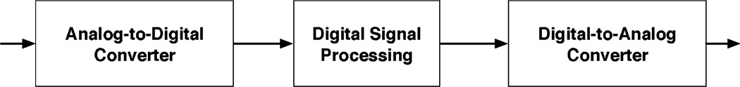
General signal processing chain with a digital signal processing core.

This ubiquitous discrete representation, however, is suboptimal for a number of critical future applications. Consider, for example, streaming video. In the classical DSP processing chain (see Fig. 1), a video frame is typically generated every 33 ms. Phenomena that operate at a time scale below the frame rate, appear blurred and interpolation algorithms have limited utility. Signal processing algorithms process every pixel even if no change has taken place. Newly implemented event driven video encoders are frame-free and provide extremely high time resolution [4]. Thus the need for choosing highly versatile representations inspired by human visual capabilities. The method of choice is to represent information in the time domain (spike domain).

Next generation encoders are expected to represent information in the time domain [32]. Representing information in the time domain is achieved via time encoding [26]. Formally, time encoding is a real-time asynchronous mechanism of mapping the amplitude of a bandlimited signal u(t), t ∈ 𝕋, into an N multidimensional time sequence $(t_k^j)$, k ∈ 𝕂 and j = 1, 2, …, N, where 𝕋 and 𝕂 denote subsets of the real numbers and integers, respectively. A time encoding machine (TEM) is the realization of an asynchronous time encoding mechanism. A time decoding machine (TDM) is the realization of an algorithm for signal recovery with arbitrary accuracy [26].

The interest in time encoding in signal processing is driven by the expected paradigm shift in the design and implementation of future analog to digital converters from information representation in the amplitude domain to information representation in the time domain. Due to the ever decreasing size of integrated circuits and the attendant low voltage, amplitude-domain high precision quantizers are more and more difficult to implement. TEMs leverage the phenomenal device speeds that a temporal code can take advantage of. The interest in temporal encoding in neuroscience is closely linked with the natural representation of sensory stimuli (signals) as a sequence of action potentials (spikes). Spikes are discrete time events that carry information about stimuli.

A signal processing chain for computing in the time domain is shown in Fig. 2. It has the same broad scope as the signal processing chain briefly described above. The TEM in Fig. 2 corresponds to the A/D converter in Fig. 1. Similarly the Time Domain Computing block in Fig. 2 corresponds to the Digital Signal Processing block in Fig. 1 and the TDM to the D/A converter.

Fig. 2.

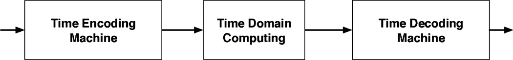
General signal processing chain with a time domain computing core.

Widely used modulation circuits such as asynchronous sigma/delta modulators and FM modulators in cascade with zero crossing detectors have been shown to be instances of TEMs [26]. TEMs based on single neuron models such as integrate-and-fire (IAF) neurons [14] have also been characterized. Multichannel TEMs realized with invertible filterbanks and invertible IAF neurons have been studied in [15]. An extensive characterization of single-input multiple-output (SIMO) TEMs can be found in [21]. A number of spike domain processing algorithms were demonstrated [16], [21], including faithful stimulus recovery. Real-time recovery algorithms were investigated in [25]. In all these works, perfect or faithful signal recovery is achieved provided that a Nyquist-type rate condition is satisfied.

We have also investigated architectures for the encoding and decoding of natural and synthetic video streams (movies, animation) and, sounds and speech. The stimuli were encoded with, e.g., a video time encoding machine [20], and subsequently faithfully decoded. We demonstrated that [20] the information contained in the video input can be recovered from the output of the video TEM provided that the number of computing elements (neurons) is beyond a threshold value. Therefore, while information about the signals can not be perfectly represented with a small number of neurons, this limitation can be overcome provided that the number of neurons is beyond a certain critical value. Increasing the number of neurons to achieve a faithful representation of the sensory world is consistent with basic neurobiological thought.

B. Background for the Theoretical Neuroscientist

In the reverse correlation method to neural encoding [30], the neural system is treated as a black box and both the input stimuli and output spike trains are assumed to be observable. Based on the correlation between the input and the output, the black box is identified as the kernel of a Wiener filter. When investigating problems arising in sensory encoding, an explicit characterization of sensory stimuli is, however, not available. Under these conditions, investigations of sensory encoding of natural stimuli need to assume that only the spike train is observable. Often, one also assumes that the neural system can be modeled as a nonlinear dynamical system.

Exploring neural encoding circuits with conductance based models is high on the research agenda. Since the bedrock of conductance based models is the Hodgkin–Huxley neuron, the later is the building block of choice in these circuits. To the best of our knowledge, formal investigations of encoding models based on a population of Hodgkin–Huxley neurons using methods of information processing are scarce in the literature. See, however, [38], [19], [6] for single neurons investigations and [18] for a study of ensemble encoding. The importance of these methods can not be, however, overstated as they provide a bridge between theoretically tractable explorations of neural encoding and lab bench experiments in systems neuroscience.

In this paper, a sensory neuron is modeled as a point neuron whose spike generation mechanism is described by the Hodgkin–Huxley equations

$$C\frac{dV}{dt}=-g_{Na}{m}^{3}h(V-E_{Na})-g_K{n}^4(V-E_K)-g_L(V-E_L)+I\frac{dm}{dt}={\alpha }_m(V)(1-m)-{\beta }_m(V)m\frac{dh}{dt}={\alpha }_h(V)(1-h)-{\beta }_h(V)h\frac{dn}{dt}={\alpha }_n(V)(1-n)-{\beta }_n(V)n$$ (1)

where V is the membrane voltage of the neuron, m, h and n are the gating variables and I is the injected current. See [36], [11] for the notation used and other pertinent model details.

In order to simplify the mathematical language, the equations above are rewritten in the standard form

$$\frac{d\mathbf{x}}{dt}=\mathbf{f}(\mathbf{x})$$ (2)

where x and f are vectors of appropriate dimensions, and x(0) = x₀ is the initial condition. These vectors can easily be identified from the set of Hodgkin–Huxley equations. In particular, x = (x₁, x₂, x₃, x₄) = (V, m, h, n). The expression for f = (f₁, f₂, f₃, f₄) can also be easily derived from the same set of equations. In what follows we shall assume that, if the (step) injected current I is in the appropriate range, the essential dynamics of this set of equations are described by a limit cycle [36], [28], [11].

C. Overview

In this paper, we investigate the recovery of stimuli encoded with sensory neuron models that arise in olfactory systems, vision and hearing [7]. Each sensory neuron is modeled as a point neuron whose spike generation mechanism is described by the Hodgkin–Huxley equations [36], [28], [11].

In previous work, inspired by circuits arising in communications, we investigated encoding with general garden variety oscillators (e.g., Hodgkin–Huxley neurons) with multiplicative coupling, feedforward and feedback. FM modulation, e.g., is based on multiplicatively coupling a signal onto a carrier. A brief characterization of these encoding methods appears in [17]. We shall review these results in Section II as they offer strong intuition for the more complex encoding circuits that follow.

More formally, we consider Hodgkin–Huxley neurons in a multiplicative and an additive coupling configuration. Multiplicative coupling of a scalar stimulus u = u(t) is of the form (see also (2)) [17], [18]

$$\frac{d\mathbf{y}}{dt}=(b+u(t))\mathbf{f}(\mathbf{y})$$ (3)

where b is a constant such that b + u(t) > 0. Additive coupling of a vector stimulus u = u(t) is of the form [19]

$$\frac{d\mathbf{y}}{dt}=\mathbf{f}(\mathbf{y})+\mathbf{B}(\mathbf{y})\mathbf{u}(t)$$ (4)

where B is a matrix of appropriate dimensions. We shall also consider Hodgkin–Huxley neurons with gating variables driven by white noise [19], i.e.,

$$d\mathbf{Y}=\mathbf{f}(\mathbf{Y})dt+\mathbf{B}(\mathbf{Y})d\mathbf{Z}(t)$$ (5)

where dZ = (udt, dW₂(t), dW₃(t), dW₄(t))^T. Here u = u(t) denotes the stimulus and W = (0, W₂(t), W₃(t), W₄(t))^T is a vector of independent Brownian motion processes. Note that for B = I (identity matrix), W appears as an input only to the state equations describing the gating variables of the Hodgkin–Huxley neuron.

A non-linear perturbation analysis shows that the system of differential (4) describing the Hodgkin–Huxley neuron with a weak stimulus accepts a solution consisting of a phase shift term and a small perturbation term. Let τ = τ(t) be a positive function, i.e., τ(t) > 0 for all t, t ∈ 𝕋. The function τ, called the phase shift process in this paper, models a time change. The system of (4) above admits a solution of the form

$$\mathbf{y}={\mathbf{x}}^o(t+\tau (t))+\mathbf{v}(t)$$

where x^o is an orbital solution to (2), the phase shift process τ satisfies a differential equation and v is a small perturbation. The interpretation of the solution above is very simple. Assuming that the system of differential (2) has an orbitally stable solution, the solution to the (4) above with weak stimulus can be characterized by a phase shift along the stable orbital trajectory and a small perturbation from this trajectory. The structure of the solution above remains the same for the Hodgkin–Huxley neuron with stochastic conductances given by (5).

We shall demonstrate that a Hodgkin–Huxley neuron with deterministic or stochastic gating variables and weak input is (first-order) I/O equivalent with a project-integrate-and-fire neuron with variable threshold. Two neurons are defined to be first order I/O equivalent if the associated sequences of interspike (or intertrigger) intervals (iS_k = t_k+1 − t_k), k ∈ 𝕂, are, to a first order, identical [18]. Here (t_k), k ∈ 𝕂, generically denotes the sequence of spike or trigger times generated by one of the neurons. The PIF neurons, a class of spiking neurons first introduced in [19] and expanded upon in this paper, integrates the projection of the input on the phase response curve. The I/O equivalence result allows us to reduce the problem of stimulus encoding with a Hodgkin–Huxley neuron to one consisting of a project-integrate-and-fire neuron with the same input stimulus.

In order to recover the signal u = u(t), t ∈ 𝕋, from the spike train (t_k), k ∈ 𝕂, the stimuli are defined in a reproducing kernel Hilbert space (RKHS). The “natural choice” of the RKHS depends on the stimuli of interst, i.e., olfactory, hearing or visual. We provide choices that are mainly determined by the properties of the PIF neuron. For Hodgkin–Huxley neurons with multiplicative coupling, the natural choice is the space of bandlimited signals, as we can show that a perfect recovery of stimuli is possible [17]. In the additive coupling case of Hodgkin–Huxley neuron models with deterministic conductances, the PIF neuron is a low noise I/O equivalent. Here we opted for a recovery algorithm based on interpolation splines [22]. The methodology of interpolation splines is closely related to signal representations using sinc functions as in the case of bandlimited stimuli above. Finally, for additively coupled Hodgkin–Huxley neurons with stochastic conductances, we give a recovery method based on smoothing splines [23].

This paper is organized as follows. The encoding of stimuli into spike trains by a Hodgkin–Huxley neuron with multiplicative coupling is investigated in Section II. The I/O equivalent neuron is an integrate-and-fire neuron. For bandlimited stimuli a perfect recovery algorithm is given in the same section. The first order I/O equivalent neuron for a Hodgkin–Huxley neuron with deterministic conductances is shown to be a project-and-fire neuron in Section III. Based on the PIF encoding model, a stimulus recovery algorithm is presented under the assumptions that stimuli have bounded energy. In Section IV the first-order I/O equivalent of a Hodgkin–Huxley neuron with stochastic conductances is derived. The I/O equivalent neuron model is a PIF with random thresholds. The same section also presents a recovery algorithm for a class of smooth stimuli. Finally, in Section V the encoding of stimuli with an ensemble of Hodgkin–Huxley neurons is investigated. An algorithm for recovering the encoded stimuli is given.

The paper assumes familiarity with elementary methods of nonlinear dynamical systems [11], [8], functional analysis [29], [3], stochastic processes [27], [33], statistics [35], [1] and approximation theory [2]. For the benefit of the reader, some of the results employed are included in the Appendix.

II. Encoding With Hodgkin–Huxley Neurons With Multiplicative Coupling

In this paper, we consider models of information representation arising in olfactory systems, vision and hearing [7]. As already mentioned, each sensory neuron is modeled as a point neuron whose spike generation mechanism is described by the Hodgkin–Huxley (1). Recall that, for a constant injected current in the admissible range, the essential dynamics of this set of equations are described by a limit cycle [36], [28], [11].

Let u = u(t) be a function defined on the finite time interval 𝕋 ⊂ ℝ and b a positive constant such that b + u(t) > 0 for all t, t ∈ 𝕋; u + b models the aggregate dendritic current entering the soma of the sensory neuron and ℝ denotes the real numbers. In what follows we shall assume that the Hodgkin–Huxley neuron is stimulated via tangential (multiplicative) coupling [17], [18], [19]. With multiplicative coupling, the input to a single neuron appears as a multiplicative term on the right hand side of the (2) above, i.e.

$$\frac{d\mathbf{y}}{dt}=(b+u(t))\mathbf{f}(\mathbf{y})$$ (6)

for some given initial condition y(0). As we shall show in the next section, in the multiplicative coupling model, the stimulus introduces a signal dependent phase shift (time change). When the stimulus is absent (u = 0), b modulates the activity of the neuron through a time change. More generally, if x = x(t) denotes the solution to the Hodgkin–Huxley neuron, the general solution in the multiplicative coupling case is $\mathbf{y}=\mathbf{x}(bt+{\int }_0^{t}u(s)ds)$ provided that y(0) = x(0). The time change is thus stimulus driven. Let 𝕂 denote the set {1, 2, …, n}.

Definition 1: Two neurons are said to be I/O equivalent if the associated sequences of intertrigger times (iS_k = t_k+1 − t_k), k ∈ 𝕂, are identical.

In the next section we shall show that a Hodgkin–Huxley neuron with multiplicative coupling is I/O equivalent with an IAF neuron with a variable threshold sequence. The values of the threshold sequence are explicitly given.

A. I/O Equivalence for Hodgkin–Huxley Neurons With Tangential Coupling

In what follows we assume that the model neuron is described by the Hodgkin–Huxley equations with multiplicative coupling. With multiplicative coupling and input u + b, the neuron is described by the systems of (6). We have the following [17].

Lemma 1: Given the initial condition y(0) = x(0),

$$\mathbf{y}=\mathbf{x}(bt+{\int }_0^{t}u(s)ds)$$ (7)

for all t, t ∈ ℝ₊, where x = x(t), t ∈ ℝ₊, is the solution to (2) starting at x(0) = x₀.

Proof: By differentiating the right hand side of (7) above, we have

$$\frac{d\mathbf{y}}{dt}=\frac{d\mathbf{x}(\upsilon )}{d\upsilon }{|}_{\upsilon =bt+{\int }_0^{t}u(s)ds}·(b+u(t))=(b+u(t))·\mathbf{f}\left(\mathbf{x}\right(bt+{\int }_0^{t}u(s)ds\left)\right)=(b+u(t))·\mathbf{f}(\mathbf{y}).$$

The assertion immediately follows since y(0) = x(0).

Remark 1: The solution to (6) is obtained from the solution to (2) via the time change $t\to bt+{\int }_0^{t}u(s)ds$. The condition b + u(t) > 0 is very natural in this light since it ensures that the changed time remains strictly increasing.

In what follows, we shall assume that the observable output of the Hodgkin–Huxley neuron comprises solely the spike times of the membrane voltage, that is, the times when the spike maxima of the coordinate x₁ are reached. Note that other definitions of spike time occurrence, e.g., zero crossings, can also be employed [18]. Thus, the spike times are a subset of the zeros of dx₁/dt (the additional condition is that the second derivative of x₁ is negative). They are denoted by (δ_k), k ∈ 𝕂. Therefore

$$\frac{d{x}_1}{dt}({\delta }_k)=0$$ (8)

for all k, k ∈ 𝕂. In what follows, the trigger times (t_k), k ∈ 𝕂, denote the spike times of y₁.

Lemma 2 (t-Transform): The sequence of trigger times (t_k), k ∈ 𝕂, and the sequence of spike times (δ_k), k ∈ 𝕂, verify the set of recursive equations

$${\int }_{t_k}^{t_{k+1}}u(s)ds={\delta }_{k+1}-{\delta }_k-b(t_{k+1}-t_k),$$ (9)

for all k, k ∈ 𝕂.

Proof: Since (δ_k), k ∈ 𝕂, is a subset of the zeros of the first derivative of x₁,

$$f_1(\mathbf{x}({\delta }_k))=0$$ (10)

and (t_k), k ∈ 𝕂, is a subset of the zeros of the first derivative of y₁

$$f_1(\mathbf{x}(b{t}_k+{\int }_0^{t_k}u(s)ds))=0$$ (11)

and the two subsets are the same, the result follows.

Equation (9) above defines the t-transform; it maps the amplitude information of (u(t)), t ∈ 𝕋, into the time sequence (t_k), k ∈ 𝕂. Thus, the information encoded by a Hodgkin–Huxley neuron with multiplicative coupling is, from a signal recovery standpoint, equivalent with the information encoded by an integrate-and-fire neuron with threshold δ_k+1 − δ_k during the time interval [t_k, t_k+1] for all k, k ∈ 𝕂. Formally, we have the following theorem.

Theorem 1 (I/O Equivalence): Assume that the variable threshold sequence of an Integrate-and-Fire neuron is identical to the interspike interval sequence (δ_k+1 − δ_k), k ∈ 𝕂, generated by a tonically spiking Hodgkin–Huxley neuron. Then the Hodgkin–Huxley neuron with multiplicative coupling and the Integrate-and-Fire neuron generate the same intertrigger interval sequence (iS_k), k ∈ 𝕂, i.e., the two neurons are input/output equivalent.

Fig. 3 shows the output of a Hodgkin–Huxley neuron with multiplicative coupling and the output of the I/O equivalent integrate-and-fire neuron. The spike times are depicted with circles.

Fig. 3.

I/O equivalence based on spike times defined as maxima.

B. Stimulus Recovery

In this section, we derive an algorithm for perfect recovery of a stimulus u = u(t), t ∈ ℝ, encoded by a Hodgkin–Huxley neuron with multiplicative coupling. The recovery algorithm is based on the knowledge of the trigger times (t_k), k ∈ ℤ. We shall assume that the stimulus u(t), t ∈ ℝ, is bounded |u| ≤ c < b and it is an element of Ξ, the space of functions bandlimited to [−Ω, Ω]. When endowed with the usual inner product, Ξ is a Reproducing Kernel Hilbert Space with the sinc kernel g(t) = sin(Ωt)/πt, t ∈ ℝ.

Let us denote by ${[\mathbf{q}]}_k={\int }_{t_k}^{t_{k+1}}u(s)ds$ and ${[\mathbf{G}]}_{lk}={\int }_{t_l}^{t_{l+1}}g(s-s_k)ds$, where s_k = (t_k+1 + t_k)/2. For simplicity we shall assume that the Hodgkin–Huxley neuron is I/O equivalent with an IAF neuron with threshold δ, i.e., δ_k+1 − δ_k = δ for k ∈ 𝕂. We have the following.

Theorem 2: If δ/b < π/Ω, the bandlimited stimulus u(t), t ∈ ℝ, encoded with an IAF neuron can be perfectly recovered from (t_k)_k∈ℤ as

$$u(t)=\sum _{k\in \mathbb{Z}}{c}_k{\psi }_k(t)$$ (12)

where ψ_k(t) = g(t − s_k) and c = G⁺q, where G⁺ denotes the pseudo-inverse of G.

Proof: The spike density (the average number of spikes over arbitrarily long time intervals) of the IAF neuron is given by b/δ [24]. Therefore, for δ/b < π/Ω the set of representation functions (ψ_k(t)), k ∈ ℤ, and t ∈ ℝ, is a frame in Ξ [3] and

$$u(t)=\sum _{k\in \mathbb{Z}}{c}_k{\psi }_k(t).$$ (13)

Furthermore, the set of sampling functions ϕ = (ϕ_k)_k∈ℤ, t ∈ ℝ, defined by

$${\varphi }_k(t)=(1_{[t_k,t_{k+1}]}*g)(t)$$

where * denotes the convolution, is also a frame in Ξ.

By applying the inner product to the representation above, we get

$$\langle u,{\varphi }_l\rangle =\sum _{k\in \mathbb{Z}}{c}_k\langle {\psi }_k,{\varphi }_l\rangle$$

and therefore with [q]_l = 〈u, ϕ_l〉 and [G]_lk = 〈ψ_k, ϕ_l〉 = 〈ϕ_l, ψ_k〉, we obtain the familiar c = G⁺ q [26], [14].

Concluding, a reader or receiver with access to the spike sequence (t_k), k ∈ ℤ, has in effect knowledge of the sequence of projections 〈u, ϕ_k〉, k ∈ ℤ. The projections 〈u, ϕ_k〉, k ∈ ℤ, are the measurements on the stimulus. If the sequence (ϕ_k), k ∈ ℤ, spans Ξ, we can, in principle, recover the stimulus u from these projections. Extensions to other classes of TEMs including feedforward and feedback can be found in [17].

Remark 2: The reconstruction formula has a simple geometric interpretation. The stimulus u ∈ Ξ is first sampled (measured) by projecting it on the sampling functions ϕ_k(t), k ∈ ℤ, and then represented with ψ_k(t), k ∈ ℤ. The sampling functions ϕ_k(t), k ∈ ℤ, are determined by the neural circuit. The set of functions ψ_k(t), k ∈ ℤ, have to represent bandlimited stimuli where in Ξ in a stable way.

III. Encoding With Hodgkin–Huxley Neurons With Deterministic Conductances

We consider in this section a Hodgkin–Huxley neuron with additive coupling described by the system of differential equations

$$\frac{d\mathbf{y}}{dt}=\mathbf{f}(\mathbf{y})+\mathbf{B}(\mathbf{y})\mathbf{u}(t)$$ (14)

where u = u(t) is the (additive) stimulus and B(y)u(t) is the perturbation. The perturbation is the “projection” of the input u onto B. Intuitively, the perturbation induced by the input u will lead to a time (phase) shift or phase deviation along the orbit and an orbital deviation. The phase shift term is due to a component of the perturbation that is tangential to the orbit. This is formalized below (see also [19], [18]).

Let x^o be an orbital solution to the system of differential (2) and let x^o(t + τ(t)) be a time shifted version of this solution.

Definition 2: A function τ = τ(t), t ∈ ℝ₊, with τ(0) = 0, such that σ(t) = t + τ(t) is strictly increasing is called a phase shift process (PSP). The function σ = σ(t), t ∈ ℝ₊, is called a time change.

Clearly, y(t) = x^o(t + τ(t)) is the solution to the system of differential equations

$$\frac{d\mathbf{y}}{dt}=(1+\frac{d\tau }{dt})\mathbf{f}(\mathbf{y})$$ (15)

with τ(0) = 0 and y(0) = x^o(0) = x₀. This suggests decomposing the response of the Hodgkin–Huxley neuron to a weak stimulus into a term along the orbit and a term accounting for a deviation from the orbit.

A. I/O Equivalence for Hodgkin–Huxley Neurons With Additive Coupling

The results invoked below appeared in literature that deals with the design and analysis of high frequency oscillators [12] and [5], the literature on nonlinear dynamical systems [10], [11] and in the theoretical neuroscience literature [31], [36]. These results have largely been independently obtained. We shall adopt the language of biology/neuroscience (phase response curves [37]).

In what follows, we shall assume that the autonomous system described by the systems of differential (2) admits a periodic (orbital) solution x^o = x^o(t) with period T, that is, x^o (t+T) = x^o(t), for all t, t ∈ 𝕋 ⊆ ℝ₊. We have the following lemma.

Lemma 3: y = x^o(t + τ(t)) is the solution to

$$\frac{d\mathbf{y}}{\mathbf{d}\mathbf{t}}=\mathbf{f}(\mathbf{y})+{\mathit{\psi }}_1^T(t+\tau (t))\mathbf{B}(\mathbf{y})\mathbf{u}(t){\mathit{\varphi }}_1(t+\tau (t))$$ (16)

where

$$\frac{d\tau }{dt}={\mathit{\psi }}_1^T(t+\tau (t))\mathbf{B}({\mathbf{x}}^o(t+\tau (t)))\mathbf{u}(t)$$ (17)

with τ(0) = 0. Here ${\mathit{\psi }}_1^T(t)$ is the transpose of the phase response curve and ${\mathit{\varphi }}_1(t)=\frac{d{\mathbf{x}}^o}{dt}$.

Proof: y = x^o(t + τ(t)) is the solution to the system of (16) if

$$\frac{d{\mathbf{x}}^o(t+\tau (t))}{dt}=\mathbf{f}({\mathbf{x}}^o(t+\tau (t)))+{\mathit{\psi }}_1^T(t+\tau (t))\mathbf{B}({\mathbf{x}}^o(t+\tau (t)))\mathbf{u}(t){\mathit{\varphi }}_1(t+\tau (t)),\text{or}(1+\frac{d\tau }{dt})\frac{d{\mathbf{x}}^o}{d\upsilon }{|}_{\upsilon =t+\tau (t)}=\mathbf{f}({\mathbf{x}}^o(t+\tau (t)))+\frac{d\tau }{dt}\frac{d{\mathbf{x}}^o}{d\upsilon }{|}_{\upsilon =t+\tau (t)}.$$

Remark 3: The phase shift process in (15) is arbitrary. In Lemma 3 a choice of the phase shift process τ = τ(t) was made in (17). Note that if the right hand side of (17) is a constant, the phase shift τ can become arbitrarily large even for small constant inputs u. The existence and uniqueness of τ is guaranteed by the existence and uniqueness theorem for differential equations. More details about the phase response curve can be found in Appendix A (see also [10]).

In what follows, we shall assume again that the observable output of the Hodgkin–Huxley neuron comprises the set of spike times of the membrane voltage, that is the times when the spike maxima of the coordinate x₁ are reached. Thus, the spike times are a subset of the zeros of $d{x}_1^o/dt$ (the additional condition is that the second derivative of x₁ is negative). They are denoted by (δ_k), k ∈ 𝕂. Therefore

$$\frac{d{x}_1^o}{dt}({\delta }_k)=0$$ (18)

for all k ∈ 𝕂. In what follows, the trigger times (t_k), k ∈ 𝕂, denote the spike times of y₁.

Lemma 4 (t-Transform): The sequence of trigger times (t_k), k ∈ 𝕂, and the sequence of spike times (δ_k), k ∈ 𝕂, verify to a first order the set of recursive equations

$$\tau (t_{k+1})-\tau (t_k)={\delta }_{k+1}-{\delta }_k-(t_{k+1}-t_k)$$ (19)

for all k, k ∈ 𝕂.

Proof: Since (δ_k), k ∈ 𝕂, is a subset of the zeros of the first derivative of $x_1^o$

$$f_1({\mathbf{x}}^o({\delta }_k))=0$$ (20)

and (t_k), k ∈ 𝕂, is a subset of the zeros of the first derivative of y₁, i.e.

$$f_1({\mathbf{x}}^o(t_k+\tau (t_k)))=0$$ (21)

provided that the deviation from the orbital solution is negligible. Therefore, for small inputs

$$t_k+\tau (t_k)={\delta }_k+{\eta }_k$$

where (η_k), k ∈ 𝕂, accounts for jitter. Since for weak stimuli the jitter is infinitesimally small, we obtain the first order equivalence

$$t_k+\tau (t_k)={\delta }_k$$

and the result follows.

Equation (19) above defines the t-transform; it maps the amplitude information of (u(t)), t ∈ 𝕋, into the time sequence (t_k), k ∈ 𝕂.

Definition 3: A neuron whose spike times (t_k), k ∈ 𝕂, verify the equation

$${\int }_{t_k}^{t_{k+1}}{\mathit{\psi }}_1^T(s+\tau (s))\mathbf{B}({\mathbf{x}}^o(s+\tau (s)))\mathbf{u}(s)ds={\delta }_{k+1}-{\delta }_k-(t_{k+1}-t_k)$$ (22)

where

$$\frac{d\tau }{dt}={\mathit{\psi }}_1^T(t+\tau (t))\mathbf{B}({\mathbf{x}}^o(t+\tau (t)))\mathbf{u}(t)$$

with τ(0) = 0, is called a project-integrate-and-fire (PIF) neuron.

On the left hand-side of (22), we recognize the “projection” of the stimulus u onto the phase response curve ψ₁ and B followed by integration. Here (δ_k+1 − δ_k), k ∈ 𝕂, represents the threshold sequence of the PIF neuron.

Theorem 3 (First Order I/O Equivalence): Assume that the variable threshold sequence of a Project-Integrate-and-Fire neuron is identical to the interspike interval sequence (δ_k+1 − δ_k), k ∈ 𝕂, generated by a Hodgkin–Huxley neuron with phase response curve ψ₁ and input projection B. Then the Hodgkin–Huxley neuron and the project-integrate-and-fire neuron generate, to the first order, the same intertrigger interval sequence (iS_k), k ∈ 𝕂, i.e., the two neurons are first order input/output equivalent.

In what follows we shall assume that the stimulus is a smooth function u = [u000]^T.

Corollary 1: Assume that the Hodgkin–Huxley neuron described by the equations

$$d\mathbf{y}=\mathbf{f}(\mathbf{y})dt+{[u(t)000]}^{T}dt$$ (23)

generates the trigger time sequence (t_k),k ∈ 𝕂. The t-transform of the I/O equivalent PIF neuron with stimulus u = u(t), t ∈ 𝕋, is given by

$${\int }_{t_k}^{t_{k+1}}{\psi }_{11}(s+\tau (s))u(s)ds={\delta }_{k+1}-{\delta }_k-(t_{k+1}-t_k)$$ (24)

where the phase shift process satisfies the differential equation

$$\frac{d\tau }{dt}={\psi }_{11}(t+\tau (t))u(t)$$ (25)

with τ(0) = 0.

With (25) we can associate an operator 𝒯 such that τ(t) = (𝒯u)(t). u satisfies, therefore, the following integral equation

$${\int }_{t_k}^{t_{k+1}}{\psi }_{11}(s+(𝒯u)(s))u(s)ds={\delta }_{k+1}-{\delta }_k-(t_{k+1}-t_k).$$ (26)

Since finding the t-transform inverse seems analytically intractable, we shall consider instead the reduced t-transform

$${\int }_{t_k}^{t_{k+1}}\phi (s)u(s)ds={\delta }_{k+1}-{\delta }_k-(t_{k+1}-t_k)$$ (27)

where φ(s) = ψ₁₁(s). This approximation is justified as long as the phase shift process changes slowly as compared to the oscillation period of the Hodgkin–Huxley neuron [34]. A neuron with the t-transform given by (27) is called a reduced PIF neuron.

B. Stimulus Recovery

In this section, we formulate and solve the problem of optimal consistent reconstruction of a stimulus encoded with a Hodgkin–Huxley neuron with deterministic conductances.Areceiver or reader of the spike train first builds an encoding model based on the reduced PIF neuron.

We show how the spike train of the reduced PIF neuron can be associated with a series of projections in the chosen space of finite length signals with bounded energy. We impose intuitive constraints on the desired reconstructed signal and show that the reconstruction algorithm can be obtained by solving a spline interpolation problem. In a second step, the receiver implements the reconstruction algorithm based on the spike train generated by the Hodgkin–Huxley neuron with deterministic conductances.

1) Neural Encoding With a PIF Neuron: Let u = u(t), t ∈ 𝕋, be a signal (or stimulus) of finite length and bounded energy, i.e., u ∈ L²(𝕋). In what follows we assume that the stimulus u is the input to a reduced PIF neuron with the t-transform given by

$${\int }_{t_k}^{t_{k+1}}\phi (s)u(s)ds=q_k$$ (28)

for all k, k = 1, 2, …, n − 1. The t-transform can be rewritten as

$$L_{k}u=q_k$$ (29)

where L_k : L²(𝕋) ↦ ℝ is a linear functional given by

$$L_{k}u={\int }_{t_k}^{t_{k+1}}\phi (s)u(s)ds$$ (30)

$$q_k={\delta }_{k+1}-{\delta }_k-(t_{k+1}-t_k)$$ (31)

for all k = 1, 2, …, n − 1. Therefore, we have the following result.

Lemma 5: The t-transform of the reduced PIF neuron can be written in inner-product form as

$$\langle u,{\varphi }_k\rangle =q_k$$ (32)

where

$${\varphi }_k(t)=\phi (t)1_{[t_k,t_{k+1}]}(t)$$ (33)

and 〈·, ·〉 : L²(𝕋)×L²(𝕋) ↦ ℝ is the standard L² inner product restricted to the domain 𝕋 for all k = 1, 2, …, n − 1.

The set of measurements or encodings expressed by the linear functionals in (29) or the projections in (32) can be readily derived from the knowledge of the spike times and the neuron parameters. Thus, through the use of the t-transform [26], we can determine both the sampling functions and the projections of the stimulus on these functions using only the knowledge of the spike times.

2) Consistent Stimulus Recovery: The problem of stimulus reconstruction calls for estimating the signal u given the set of spikes (t_k), k = 1, 2, …, n. This problem is, for the class of stimuli u ∈ L²(𝕋) ill-defined. A remedy is provided by introducing a set of constraints on the recovery. The first constraint considered here requires the reconstructed signal û to generate the same spikes as the original stimulus. The second constraint requires choosing among the reconstructed stimuli the one with the maximum degree of smoothness. The latter is formulated as an optimization criterion. The presentation below closely follows [22].

Definition 4: A reconstruction û of u based on the spike times (t_k), k = 1, 2, …, n, is said to be consistent if û triggers exactly the same spike train as the original stimulus u.

Remark 4: Assume that at time 0 the membrane potential of the reduced PIF neuron is set to the resting potential 0. Then the consistency condition above is equivalent with

$$\langle u,{\varphi }_k\rangle =\langle \widehat{u},{\varphi }_k\rangle$$ (34)

for all k, k = 1, 2, …, n − 1.

Definition 5: A consistent reconstruction û that minimizes the quadratic criterion

$$\Vert Ju\Vert ={\left({\int }_{𝕋}{\left(\frac{d^{2}u}{d{s}^2}\right)}^{2}ds\right)}^{1/2}$$ (35)

is called the optimal consistent reconstruction of u.

Lemma 6: The optimal consistent reconstruction û solves the spline interpolation problem

$$\widehat{u}=\underset{\langle u,{\varphi }_k\rangle =q_k}{\text{argmin}}\Vert \frac{d^{2}u}{d{s}^2}\Vert$$ (36)

where ‖·‖ is the standard L²-norm restricted to the interval 𝕋.

Proof: Follows directly from Definitions 4 and 5.

Remark 5: An introduction to splines and the general solution to spline interpolation problems is presented in the Appendix B.

Theorem 4: The optimal consistent reconstruction of a stimulus encoded with a reduced PIF neuron is unique and is given by

$$\widehat{u}(t)=d_0+d_{1}t+\sum _{k=1}^{n-1}{c}_k{\psi }_k(t)$$ (37)

where

$${\psi }_k(t)=({\varphi }_k*{|·|}^3)(t)$$ (38)

and |·| denotes the absolute value. With c = [c₁, c₂, …, c_n−1]^T, d = [d₀, d₁] and q = [q₁, q₂, …, q_n−1]^T the coefficients c and d satisfy the matrix equations

$$\left[\begin{array}{ccc}\hfill \mathbf{G}\hfill & \hfill \mathbf{p}\hfill & \hfill \mathbf{r}\hfill \\ \hfill {\mathbf{p}}^T\hfill & \hfill 0\hfill & \hfill 0\hfill \\ \hfill {\mathbf{r}}^T\hfill & \hfill 0\hfill & \hfill 0\hfill \end{array}\right]\left[\begin{array}{c}\hfill \mathbf{c}\hfill \\ \hfill d_0\hfill \\ \hfill d_1\hfill \end{array}\right]=\left[\begin{array}{c}\hfill \mathbf{q}\hfill \\ \hfill 0\hfill \\ \hfill 0\hfill \end{array}\right].$$ (39)

Moreover G is an (n − 1) × (n − 1) matrix and p, r are column vectors with entries given by

$${[\mathbf{G}]}_{kl}=\langle {\varphi }_k,{\psi }_l\rangle {[\mathbf{p}]}_k=\langle {\varphi }_k,1\rangle {[\mathbf{r}]}_k=\langle {\varphi }_k,t\rangle .$$ (40)

Proof: The proof follows from Theorem 9 in Appendix B originally published in [22]. Note that the function |·|³ is up to a multiplicative constant the Green’s function for the second-order-iterated Laplacian.

IV. Encoding With Hodgkin–Huxley Neurons With Stochastic Conductances

In what follows, we shall characterize the phase shift process when the Hodgkin–Huxley neuron is driven by a deterministic stimulus and the gating variables are driven by white noise, i.e., in the additive coupling mode

$$d\mathbf{Y}=\mathbf{f}(\mathbf{Y})dt+\mathbf{B}(\mathbf{Y})d\mathbf{Z}(t)$$ (41)

where dZ = (udt, dW₂(t), dW₃(t), dW₄(t))^T. Furthermore u = u(t) denotes the stimulus and W = (0, W₂(t), W₃(t), W₄(t))^T is a vector of independent Brownian motion processes. For B = I, W appears as an input only to the state equations describing the gating variables of the Hodgkin–Huxley neuron. For questions regarding the existence and uniqueness of solutions for stochastic differential equations the reader should consult [33], [27], [8].

A. First Order I/O Equivalence for the HHN With Stochastic Conductances

The PSP satisfies the stochastic differential equation

$$d\tau ={\mathit{\psi }}_1^T(t+\tau (t))\mathbf{B}({\mathbf{x}}^o(t+\tau (t)))d\mathbf{Z}(t)$$ (42)

with τ(0) = 0. Clearly, τ = (τ(t)), t ∈ 𝕋 ⊆ ℝ₊, is a stochastic process. For a more detailed discussion, see [34].

In what follows we shall assume that the observable output of the Hodgkin–Huxley neuron is the coordinate x₁, that is, the membrane voltage at spike times. The spike times of the membrane voltage are defined here as the maxima of x₁. Thus, the spike times are a subset of the zeros of dx₁/dt (the additional condition is that the second derivative of x₁ is negative). They are denoted by (δ_k), k ∈ 𝕂. Therefore

$$\frac{d{x}_1^o}{dt}{|}_{t={\delta }_k}=0$$

for all k ∈ 𝕂. In what follows, the trigger times (t_k), k ∈ 𝕂, denote the spike times of Y₁, i.e.

$$\frac{d{Y}_1}{dt}{|}_{t=t_k}=0.$$

Lemma 7: (t-Transform) The sequence of trigger times (t_k), k ∈ 𝕂, and the sequence of spike times (δ_k), k ∈ 𝕂, verify, to a first order, the set of recursive equations

$$\tau (t_{k+1})-\tau (t_k)={\delta }_{k+1}-{\delta }_k-(t_{k+1}-t_k)$$ (43)

for all k, k ∈ 𝕂.

Proof: We recall that (δ_k), k ∈ 𝕂, is a subset of the zeros of the first derivative of $x_1^o$

$$f_1({\mathbf{x}}^o({\delta }_k))=0$$

and (t_k), k ∈ 𝕂, is a subset of the zeros of the first derivative of Y₁

$$f_1({\mathbf{x}}^o(t_k+\tau (t_k)))=0$$

provided that the perturbation induces a change in the vector field mainly along the orbital solution. Assuming that the perturbation is small, and since the two zero subsets are the same, we have

$$t_k+\tau (t_k)={\delta }_k+{\epsilon }_k$$

where (ε_k), k ∈ 𝕂, accounts for random jitter. For infinitesimal perturbations the random jitter is arbitrarily small and the result follows.

Equation (43) above defines the t-transform of a neuron observed at its spike times; it maps the amplitude information of (u(t)), t ∈ 𝕋, into the time sequence (t_k), k ∈ 𝕂.

Definition 6: A neuron whose spike times (t_k), k ∈ 𝕂, verify the equation

$${\int }_{t_k}^{t_{k+1}}{\mathit{\psi }}_1^T(s+\tau (s))\mathbf{B}({\mathbf{x}}^o(s+\tau (s)))d\mathbf{Z}(s)={\delta }_{k+1}-{\delta }_k-(t_{k+1}-t_k)$$ (44)

where

$$d\tau ={\mathit{\psi }}_1^T(t+\tau (t))\mathbf{B}({\mathbf{x}}^o(t+\tau (t)))d\mathbf{Z}(t)$$ (45)

with τ(0) = 0, is called a project-integrate-and-fire (PIF) neuron with random thresholds.

Remark 6: The systems of (44) and (45) describing the PIF neuron are stochastic. Consequently, the threshold of the neuron is random. The structure of the PIF neuron will be further analyzed below.

Theorem 5: (First-Order I/O Equivalence) Assume that the variable threshold sequence of a project-integrate-and-fire neuron is identical to the interspike interval sequence (δ_k+1 − δ_k), k ∈ 𝕂, generated by a Hodgkin–Huxley neuron with phase response curve ψ₁ and input projection B. Then the Hodgkin–Huxley neuron and the project-integrate-and-fire neuron generate, to the first order, the same intertrigger interval sequence (iS_k), k ∈ 𝕂, i.e., the two neurons are first order input/output equivalent.

In what follows, we shall assume for simplicity that B = I and the vector Brownian motion W = (0, W₂(t), W₃(t), W₄(t))^T. Thus the t-transform is of the form

$${\int }_{t_k}^{t_{k+1}}{\psi }_{11}(s+\tau (s))u(s)ds={\delta }_{k+1}-{\delta }_k-(t_{k+1}-t_k)-{\int }_{t_k}^{t_{k+1}}{\psi }_{12}(s+\tau (s))d{W}_2(s)-{\int }_{t_k}^{t_{k+1}}{\psi }_{13}(s+\tau (s))d{W}_3(s)-{\int }_{t_k}^{t_{k+1}}{\psi }_{14}(s+\tau (s))d{W}_4(s).$$

Therefore, in order to recover the stimulus u, we need to develop a methodology that takes into account the noisy observations.

Corollary 2: Assume that the Hodgkin–Huxley neuron is described by the equations:

$$d\mathbf{Y}=\mathbf{f}(\mathbf{Y})dt+{[u(t)000]}^{T}dt+{[0d{W}_{2}d{W}_{3}d{W}_4]}^T$$ (46)

with trigger time sequence (t_k), k ∈ 𝕂. The t-transform of the I/O equivalent PIF neuron with random thresholds and input stimulus u = u(t), t ∈ 𝕋 is given by

$${\int }_{t_k}^{t_{k+1}}{\psi }_{11}(s+\tau (s))u(s)ds={\delta }_{k+1}-{\delta }_k-(t_{k+1}-t_k)-{\int }_{t_k}^{t_{k+1}}{\psi }_{12}(s+\tau (s))d{W}_2(s)-{\int }_{t_k}^{t_{k+1}}{\psi }_{13}(s+\tau (s))d{W}_3(s)-{\int }_{t_k}^{t_{k+1}}{\psi }_{14}(s+\tau (s))d{W}_4(s)$$ (47)

where the phase shift process satisfies the stochastic differential equation:

$$d\tau ={\psi }_{11}(t+\tau (t))u(t)dt+{\psi }_{12}(s+\tau (s))d{W}_2(s)+{\psi }_{13}(s+\tau (s))d{W}_3(s)+{\psi }_{14}(s+\tau (s))d{W}_4(s)$$ (48)

with τ(0) = 0.

Proof: Equations (47) and (48) are simply instantiations of the I/O equivalent PIF. The input to both is u = [u 000]^T.

With (48) we can associate an operator 𝒯 such that τ(t) = (𝒯u)(t). u satisfies, therefore, the following integral equation:

$${\int }_{t_k}^{t_{k+1}}{\psi }_{11}(s+(𝒯u)(s))u(s)ds={\delta }_{k+1}-{\delta }_k-(t_{k+1}-t_k)-{\int }_{t_k}^{t_{k+1}}{\psi }_{12}(s+(𝒯u)(s))d{W}_2(s)-{\int }_{t_k}^{t_{k+1}}{\psi }_{13}(s+(𝒯u)(s))d{W}_3(s)-{\int }_{t_k}^{t_{k+1}}{\psi }_{14}(s+(𝒯u)(s))d{W}_4(s).$$ (49)

This is exactly the t-transform compactly defining the PIF neuron with random threshold. Since finding the t-transform inverse seems analytically intractable, we shall consider the t-transform

$${\int }_{t_k}^{t_{k+1}}{\psi }_{11}(s)u(s)ds={\delta }_{k+1}-{\delta }_k-(t_{k+1}-t_k)-{\int }_{t_k}^{t_{k+1}}{\psi }_{12}(s)d{W}_2(s)-{\int }_{t_k}^{t_{k+1}}{\psi }_{13}(s)d{W}_3(s)-{\int }_{t_k}^{t_{k+1}}{\psi }_{14}(s)d{W}_4(s)$$ (50)

for all k, k ∈ 𝕂, instead. This approximation is justified as long as the phase shift process changes slowly as compared to the oscillation period of the Hodgkin–Huxley neuron [34]. We note that the random variables $({\int }_{t_k}^{t_{k+1}}{\psi }_{1m}(s)d{W}_m(s))$, m = 2, 3, 4, are conditionally independent Gaussian with conditional mean

$$𝔼{\int }_{t_k}^{t_{k+1}}{\psi }_{1m}(s)d{W}_m(s)=0$$

and variance

$$𝔼{\int }_{t_k}^{t_{k+1}}{\psi }_{1m}(s)d{W}_m(s){\int }_{t_k}^{t_{k+1}}{\psi }_{1m}(s)d{W}_m(s)={\int }_{t_k}^{t_{k+1}}{[{\psi }_{1m}(s)]}^{2}ds$$

for all m, m = 2, 3, 4, and known spike times t_k, t_k+1. Thus, the t-transform of the PIF with random thresholds can be written

$${\int }_{t_k}^{t_{k+1}}{\psi }_{11}(s)u(s)ds={\delta }_{k+1}-{\delta }_k-(t_{k+1}-t_k)+{\epsilon }_k$$

where (ε_k), k ∈ 𝕂, is a sequence of independent Gaussian random variables with zero conditional mean and variance

$$𝔼{[{\epsilon }_k]}^2=\sum _{m=2}^4{\int }_{t_k}^{t_{k+1}}{[{\psi }_{1m}(s)]}^{2}ds.$$

By dividing both sides of the t-transform with (𝔼[ε_k]²)^1/2, the resulting random variable on the right-hand side has unit variance. Therefore, we obtain the normalized noisy t-transform:

$${\int }_{t_k}^{t_{k+1}}{\phi }_k(s)u(s)ds=q_k+{\epsilon }_k$$ (51)

where

$${\phi }_k(s)=\frac{{\psi }_{11}(s)}{{(𝔼{[{\epsilon }_k]}^2)}^{1/2}}\text{and}{q}_k=\frac{{\delta }_{k+1}-{\delta }_k-(t_{k+1}-t_k)}{{(𝔼{[{\epsilon }_k]}^2)}^{1/2}}$$ (52)

and, by abuse of notation, (ε_k), k ∈ 𝕂, is a sequence of independent Gaussian random variables with zero mean and variance equal to one. A neuron with the t-transform given by (51) and (52) is called a reduced PIF neuron with random thresholds.

B. Stimulus Recovery

In this section we formulate and solve the problem of optimal reconstruction of a stimulus encoded with a Hodgkin–Huxley neuron with stochastic conductances. A receiver or reader of the spike train first builds an encoding model based on the reduced PIF neuron with random thresholds.

We show how the spike train of the reduced PIF neuron with random thresholds can be associated with a series of projections in the chosen stimulus space. We require the desired reconstructed signal to minimize an appropriate cost functional and show that the reconstruction algorithm is the solution to a regularization problem. In a second step, the receiver implements the reconstruction algorithm using the spike train generated by the Hodgkin–Huxley neuron with stochastic conductances.

1) Encoding of Stimuli With a PIF Neuron With Random Thresholds: Let u = u(t), t ∈ 𝕋, denote a stimulus in the Sobolev space 𝒮_m, m ∈ ℕ (see also Appendix C). Between two consecutive spike times the operation of the reduced PIF neuron is fully described by

$${\int }_{t_k}^{t_{k+1}}{\phi }_k(s)u(s)ds=q_k+{\epsilon }_k$$ (53)

where q_k + ε_k is interpreted as the value of the random threshold during the interspike interval [t_k, t_k+1). The t-transform can also be rewritten as

$$L_{k}u=q_k+{\epsilon }_k$$ (54)

where L_k : 𝒮_m ↦ ℝ is a linear functional given by

$$L_{k}u={\int }_{t_k}^{t_{k+1}}{\phi }_k(s)u(s)ds.$$ (55)

The sequence (L_k), k = 1, 2, …, n, has a simple interpretation; it represents the set of n noisy measurements (encodings) performed on the stimulus u. Let K(t, s) be the reproducing kernel of the chosen Sobolev space (see also (88) in Appendix C).

Lemma 8: The t-transform of the reduced PIF neuron with random thresholds can be written in inner-product form as

$$\langle {\varphi }_k,u\rangle =q_k+{\epsilon }_k$$ (56)

where

$${\varphi }_k(t)={\int }_{t_k}^{t_{k+1}}K(t,s){\phi }_k(s)ds$$ (57)

q_k is given by (52), k = 1, 2, …, n, and 〈·, ·,〉 is the inner product (87) for the space 𝒮_m, m ∈ ℕ. In addition the ε_k’s are i.i.d. Gaussian random variables with mean zero and variance 1for all k = 1, 2, …, n.

Proof: We shall rewrite the linear functionals of (54) in inner product form, i.e., as projections in 𝒮_m. The existence of an inner product form representation is guaranteed by the Riesz lemma (see, for example, [23]). Thus, there exists a set of functions ϕ_k ∈ 𝒮_m, such that

$$L_{k}u=\langle {\varphi }_k,u\rangle$$

for all k = 1, 2, …, n. Since 𝒮_m is a RKHS, we also have that

$${\varphi }_k(t)=\langle {\varphi }_k,K_t\rangle =L_k{K}_t={\int }_{t_k}^{t_{k+1}}K(t,s){\phi }_k(s)ds$$

where K_t(·) = K(·, t), for all t ∈ 𝕋.

2) Reconstruction of Stimuli in Sobolev Spaces: As shown in Section IV-B1, a PIF neuron with random threshold provides the reader with the set of measurements

$$\langle {\varphi }_k,u\rangle =q_k+{\epsilon }_k$$ (58)

where ϕ_k ∈ 𝒮_m for all k = 1, 2, …, n. Furthermore, (ε_k), k = 1, 2, …, n, are independent and identically distributed (i.i.d.) Gaussian random variables with zero mean and variance 1. The presentation below closely follows [23].

An optimal estimate û of u minimizes the cost functional

$$\frac{1}{n}\sum _{k=1}^n{(q_k-\langle {\varphi }_k,u\rangle )}^2+\lambda {\Vert {𝒫}_{1}u\Vert }^2$$ (59)

where 𝒫₁ : 𝒮_m ↦ ℋ₁ is the projection of the Sobolev space 𝒮_m to ℋ₁. Intuitively, the nonnegative parameter λ regulates the choice of the estimate û between faithfulness to data fitting (λ small) and maximum smoothness of the recovered signal (λ large). Details about the RKHS ℋ₁ and its reproducing kernel K¹ (t, s) can be found in Appendix C. We have the following result [23].

Theorem 6: Assume that the stimulus u = u(t), t ∈ [0, 1], is encoded into a time sequence (t_k), k = 1, 2, …, n, with a reduced PIF neuron with random threshold that is fully described by (53). The optimal estimate û of u is given by

$$\widehat{u}=\sum _{i=1}^m{d}_i{\chi }_i+\sum _{k=1}^n{c}_k{\psi }_k$$ (60)

where

$${\chi }_i(t)=\frac{t^{i-1}}{(i-1)!}{\psi }_k(t)={\int }_{t_k}^{t_{k+1}}{K}^1(t,s){\phi }_k(s)ds$$ (61)

and the coefficients [c]_k = c_k and [d]_i = d_i satisfy the matrix equations

$$(\mathbf{G}+n\lambda \mathbf{I})\mathbf{c}+\mathbf{F}\mathbf{d}=\mathbf{q}\mathbf{F}\prime \mathbf{c}=\mathbf{0}$$ (62)

with [G]_kl = 〈ψ_k, ψ_l〉, [F]_ki = 〈ϕ_k, χ_i〉 and [q]_k = q_k, for all k, l = 1, 2, …, n, and i = 1, 2, …, m.

Proof: Since the inner product 〈ϕ_k, u〉 describes the measurements performed by the PIF neuron with random thresholds described by (53), the minimizer of (59) is exactly the optimal estimate of u encoded into the time sequence (t_k), k = 1, 2, …, n. The rest of the proof is given in [23].

The representation functions ψ_k are given by

$${\psi }_k(t)={𝒫}_1{\varphi }_k=\langle {𝒫}_1{\varphi }_k,K_t\rangle =\langle {\varphi }_k,{𝒫}_1{K}_t\rangle =L_k{K}_t^1={\int }_{t_k}^{t_{k+1}}{K}^1(t,s){\phi }_k(s)ds.$$ (63)

Finally, the entries of the matrices F and G are given by

$${[\mathbf{F}]}_{ki}={\int }_{t_k}^{t_{k+1}}{\chi }_i(s){\phi }_k(s)ds{[\mathbf{G}]}_{kl}=\langle {\psi }_k,{\psi }_l\rangle ={\int }_{𝕋}{\psi }_k^{(m)}(s){\psi }_l^{(m)}(s)ds$$ (64)

for all k, l = 1, 2, …, n, and i = 1, 2, …, m. The systems of (62) is identical to the one described in Theorem 1 in [23].

Algorithm 1: The coefficients c and d satisfying the system of (62) are given by

$$\mathbf{c}={\mathbf{M}}^{-1}(\mathbf{I}-\mathbf{F}{(\mathbf{F}\prime {\mathbf{M}}^{-1}\mathbf{F})}^{-1}\mathbf{F}\prime {\mathbf{M}}^{-1})\mathbf{q}\mathbf{d}={(\mathbf{F}\prime {\mathbf{M}}^{-1}\mathbf{F})}^{-1}\mathbf{F}\prime {\mathbf{M}}^{-1}\mathbf{q}$$ (65)

with M = G + nλI.

Proof: The exact form of the coefficients above is derived in [23].

V. Ensemble Encoding With Hodgkin–Huxley Neurons

The complexity of the Hodgkin–Huxley formalism is daunting both from the information representation and from the stimulus recovery standpoint. This complexity is compounded when information is encoded with an ensemble of Hodgkin–Huxley neurons.

As we have shown in Section II, in the multiplicative (tangential) case, a Hodgkin–Huxley neuron is I/O equivalent with an integrate-and-fire neuron with a variable threshold sequence. This result can easily be generalized to the case when the same stimulus is represented with an ensemble of independent Hodgkin–Huxley neurons. This allows us to reduce the information representation with N Hodgkin–Huxley neurons to one with the same number of IAF neurons. An algorithm for stimulus recovery based on the spike train generated by an arbitrary subset of Hodgkin–Huxley neurons is provided in [18], [21] and will not be repeated here.

For simplicity, the rest of this section will only focus on encoding of stimuli with an ensemble of Hodgkin–Huxley neurons with stochastic conductances in the additive coupling configuration. In view of the results in Section III, encoding of stimuli with an ensemble of Hodgkin–Huxely neurons with deterministic conductances can be similarly treated. As in Section III, the recovery algorithm will be based on interpolation splines (appropriately extended to the population case).

A. Ensemble Encoding With Hodgkin–Huxley Neurons With Stochastic Conductances

The t-transform of the reduced PIF neuron that is I/O equivalent to a Hodgkin–Huxley neuron with stochastic conductances is given by

$${\int }_{t_k^i}^{t_{k+1}^i}{\psi }_{11}^i(s)u(s)ds={\delta }_{k+1}^i-{\delta }_k^i-(t_{k+1}^i-t_k^i)-{\int }_{t_k^i}^{t_{k+1}^i}{\psi }_{12}^i(s)d{W}_2^i(s)-{\int }_{t_k^i}^{t_{k+1}^i}{\psi }_{13}^i(s)d{W}_3^i(s)-{\int }_{t_k^i}^{t_{k+1}^i}{\psi }_{14}^i(s)d{W}_4^i(s)$$ (66)

for all i, i = 1, 2, …, N. As in Section IV.B1, the stimulus u = u(t), t ∈ 𝕋, is an element of the Sobolev space 𝒮_m, m ∈ ℕ.

We note that the random variables $({\int }_{t_k^i}^{t_{k+1}^i}{\psi }_{1m}^i(s)d{W}_m^i(s))$, m = 2, 3, 4, and i = 1, 2, …, N, are conditionally independent Gaussian with conditional mean

$$𝔼{\int }_{t_k^i}^{t_{k+1}^i}{\psi }_{1m}^i(s)d{W}_m^i(s)=0$$

and conditional variance

$$𝔼{\int }_{t_k^i}^{t_{k+1}^i}{\psi }_{1m}^i(s)d{W}_m^i(s){\int }_{t_k^i}^{t_{k+1}^i}{\psi }_{1m}^i(s)d{W}_m^i(s)={\int }_{t_k^i}^{t_{k+1}^i}{[{\psi }_{1m}^i(s)]}^{2}ds.$$

for all m, m = 2, 3, 4, and known spike times $t_k^i,t_{k+1}^i$. Thus, the t-transform of PIF can be written

$${\int }_{t_k^i}^{t_{k+1}^i}{\psi }_{11}^i(s)u(s)ds={\delta }_{k+1}^i-{\delta }_k^i-(t_{k+1}^i-t_k^i)+{\epsilon }_k^i$$

where $({\epsilon }_k^i)$, k ∈ 𝕂, i = 1, 2, …, N, is an array of independent Gaussian random variables with zero conditional mean and variance

$$𝔼{\epsilon }_k^i=\sum _{m=2}^4{\int }_{t_k^i}^{t_{k+1}^i}{[{\psi }_{1m}^i(s)]}^{2}ds.$$

As before we shall normalize the t-transform to

$${\int }_{t_k^i}^{t_{k+1}^i}{\phi }_k^i(s)u(s)ds=q_k^i+{\epsilon }_k^i$$

where

$${\phi }_k^i(s)=\frac{{\psi }_{11}^i(s)}{{(𝔼{[{\epsilon }_k^i]}^2)}^{1/2}}\text{and}{q}_k^i=\frac{{\delta }_{k+1}^i-{\delta }_k^i-(t_{k+1}^i-t_k^i)}{{(𝔼{[{\epsilon }_k^i]}^2)}^{1/2}}$$ (67)

and, by abuse of notation, $({\epsilon }_k^i)$, k ∈ 𝕂, is a sequence of independent Gaussian random variables with zero mean and variance equal to one, for all i, i = 1, 2, …, N.

B. Ensemble Recovery

In this section, we formulate and solve the problem of optimal reconstruction of a stimulus encoded with a population of Hodgkin–Huxley neurons with stochastic conductances. A receiver or reader of the multidimensional spike train first builds a population encoding model based on reduced PIF neurons with random thresholds.

As in Section IV-B we require the desired reconstructed signal to minimize an appropriate cost functional and show that the reconstruction algorithm is the solution to a regularization problem. In a second step, the receiver implements the reconstruction algorithm using the multidimensional spike train generated by the population of Hodgkin–Huxley neurons.

1) Encoding of Stimuli With a Population of PIF Neurons: We consider a population of N reduced PIF neurons with random thresholds. Whenever the membrane potential reaches its threshold value, the neuron j fires a spike and resets its membrane potential to 0. Let $t_k^j$ denote the k-th spike of neuron j, with k = 1, 2, …, n_j + 1. Here n_j + 1 denotes the number of spikes that neuron j triggers, j = 1, 2, …, N.

The t-transform of each neuron j is given by (see also (53))

$${\int }_{t_k^j}^{t_{k+1}^j}{\phi }_k^{j}u(s)ds=q_k^j+{\epsilon }_k^j$$ (68)

for all k = 1, 2, …, n_j, and j = 1, 2, …, N.

Lemma 9: The t-transform of the population of reduced PIF neurons with random thresholds can be written in inner product form as

$$\langle {\varphi }_k^j,u\rangle =q_k^j+{\epsilon }_k^j,$$ (69)

with ${\varphi }_k^j$ essentially given by (57) (with an added superscript ^j), $q_k^j$ given by (67), and the ${\epsilon }_k^j’\mathrm{s}$ are i.i.d. Gaussian random variables with mean zero and variance one for all and k = 1, 2, …, n_j, and j = 1, 2, …, N.

Proof: Largely the same as the Proof of Lemma 8.

2) Reconstruction of Stimuli in Sobolev Spaces: Let u = u(t), t ∈ 𝕋, be a stimulus in the Sobolev space 𝒮_m, m ∈ ℕ. In what follows our presentation below closely follows [23]. An optimal estimate û of u is obtained by minimizing the cost functional

$$\frac{1}{n}\sum _{j=1}^N\sum _{k=1}^{n_j}{(q_k^j-\langle {\varphi }_k^j,u\rangle )}^2+\lambda {\Vert {𝒫}_{1}u\Vert }^2$$ (70)

where $n={\sum }_{j=1}^N{n}_j$ and 𝒫₁ : 𝒮_m ↦ ℋ₁ is the projection of the Sobolev space 𝒮_m to ℋ₁. In what follows q denotes the column vector q = [q¹, …, q^N]′ with ${[{\mathbf{q}}^j]}_k=q_k^j$, for all j = 1, 2, …, N, and all k = 1, 2, …, n_j. We have the following result [23].

Theorem 7: Assume that the stimulus u = u(t), t ∈ [0, 1], is encoded into a time sequence $(t_k^j)$, j = 1, 2, …, N, k = 1, 2, …, n_j, with a population of reduced PIF neurons with random thresholds that is fully described by (68). The optimal estimate û of u is given by

$$\widehat{u}=\sum _{i=1}^m{d}_i{\chi }_i+\sum _{j=1}^N\sum _{k=1}^{n_j}{c}_k^j{\psi }_k^j,$$ (71)

where

$${\chi }_i(t)=\frac{t^{i-1}}{(i-1)!}{\psi }_k^j(t)={\int }_{t_k^j}^{t_{k+1}^j}{K}^1(t,s){\phi }_k^j(s)ds$$ (72)

and the coefficients vectors c = [c¹, …, c^N]′ with ${[{\mathbf{c}}^j]}_k=c_k^j$, for all j = 1, 2, …, N, and all k = 1, 2, …, n_j, and [d]_i = d_i, for all i = 1, 2, …, m, satisfy the matrix equations

$$(\mathbf{G}+\lambda \sum _{j=1}^N{n}_j·\mathbf{I})\mathbf{c}+\mathbf{F}\mathbf{d}=\mathbf{q}\mathbf{F}\prime \mathbf{c}=0$$ (73)

where G is a block square matrix defined as

$$\mathbf{G}=\left[\begin{array}{ccc}\hfill {\mathbf{G}}^{\mathbf{11}}\hfill & \hfill \mathbf{\dots }\hfill & \hfill {\mathbf{G}}^{\mathbf{1}\mathbf{N}}\hfill \\ \hfill \mathbf{⋮}\hfill & \hfill \mathbf{\ddots }\hfill & \hfill \mathbf{⋮}\hfill \\ \hfill {\mathbf{G}}^{\mathbf{N}\mathbf{1}}\hfill & \hfill \mathbf{\dots }\hfill & \hfill {\mathbf{G}}^{\mathbf{N}\mathbf{N}}\hfill \end{array}\right]\text{with}{[{\mathbf{G}}^{ij}]}_{kl}=\langle {\psi }_k^i,{\psi }_l^j\rangle$$

for all i, j = 1, …, N, all k = 1, …, n_i, and all l = 1, …, n_j, and the vector F is a column matrix defined as F = [F¹, …, F^N]′ with ${[{\mathbf{F}}^j]}_{ki}=\langle {\varphi }_k^j,{\chi }_i\rangle$, for all j = 1, 2, …, N, all k = 1, 2, …, n_j, and all i = 1, 2, …, m.

Proof: The noise terms

$$q_k^j-\langle {\varphi }_k^j,u\rangle$$

that appear in the cost functional (70) are independent Gaussian random variables with zero mean and variance 1. The rest of the proof follows from [23].

VI. Conclusion and Outlook

We recovered stimuli encoded with a population of Hodgkin–Huxley neurons. The basic Hodgkin–Huxley model is based on the assumption that the neuron is described by a limit cycle and that the stimulus causes only a small deviation from the unperturbed system. Three classes of neural encoders have been considered and presented in order of their perceived complexity.

First, we described a Hodgkin–Huxley neuron with multiplicative coupling. Such a neuron is I/O equivalent with an integrate-and-fire neuron. The threshold sequence of the IAF neuron is given by the set of interspike times of the Hodgkin–Huxley neuron with unit input. For bandlimited stimuli encoded with a Hodgkin–Huxley neuron with multiplicative coupling a perfect recovery can be achieved provided that a Nyquist rate condition is satisfied. This result is closely related to the classical Shannon sampling theorem in signal processing. However, neurons operate asynchronously, and thus at least from a methodological viewpoint, results in irregular sampling theory are most closely related.

Second, we considered a Hodgkin–Huxley neuron with additive coupling and deterministic conductances. In this case the system of ordinary differential equations describing the Hodgkin–Huxley neuron accepts a solution consisting of a phase shift term and a small perturbation term. We showed that the Hodgkin–Huxley neuron with deterministic gating variables is I/O equivalent with a project-integrate-and-fire (PIF) neuron with a variable threshold sequence. The PIF neuron integrates a projection of the stimulus onto the phase response curve that is, in turn, modulated by a phase shift process. The phase shift process is described by a differential equation that is stimulus driven. The PIF neuron generates a spike whenever a threshold value is achieved; the values of the threshold sequence are explicitly given. The recovery was formulated using a spline interpolation method in the space of finite length bounded energy signals.

Third, we investigated a Hodgkin–Huxley neuron with additive coupling and stochastic conductances. Here the first-order I/O equivalent neuron turned out to be a PIF neuron with random thresholds. The stimuli were modeled as elements of Sobolev spaces that are analytically tractable and have desirable smoothness properties. The reconstruction was based on finding a stimulus that minimizes a regularized quadratic optimality criterion.

Fourth, all previous recovery results of stimuli encoded with Hodgkin–Huxley neurons with multiplicative and additive coupling, and deterministic and stochastic conductances were extended to stimuli encoded with a population of Hodgkin–Huxley neurons.

The work presented here opens new avenues of research including 1) real-time algorithms for stimulus recovery, and 2) finding performance bounds for jitter and error recovery. Extensions to a family of conditional phase response curves [13] will be discussed elsewhere.

Biography

Aurel A. Lazar (S’77–M’80–SM’90–F’93) is a Professor of Electrical Engineering at Columbia University, New York. In the mid-1980s and 1990s, he pioneered investigations into networking games and programmable networks (www.ee.columbia.edu/aurel/networking.html). In addition, he conducted research in broadband networking with quality of service constraints; and also in architectures, network management, and control of telecommunications networks. His current research interests (www.bionet.ee.columbia.edu) are at the intersection of computational neuroscience, information/communications theory, and systems biology. In silico, his focus is on time encoding and information representation in sensory systems, and spike processing and neural computation in the cortex. In vivo, his focus is on the olfactory system of the Drosophila.

APPENDIX

A. The Phase Response Curve and Its Evaluation

There are two methods of computing the phase response curve. The first method is based on simulations. It can be used for arbitrarily large perturbations, even if the next spike is delayed by more than the length of one cycle. In the latter case, the term delay might be confusing [9], [11]. More formally, one seeks the solutions to

$$\frac{d\mathbf{x}}{dt}=\mathbf{f}(\mathbf{x})+\mathbf{I}·A\delta (t-\theta )$$

and designates the phase delay or advance of the orbital solution as the value of the phase response curve for a given phase θ (see Fig. 4).

Fig. 4.

Phase response curve for the Hodgkin–Huxley neuron.

The second method is based on using the adjoint system [11]. This method is mathematically rigorously defined. It is, restricted however, to small perurbations. The phase response curve is central to the investigations of the encoding of stimuli with Hodgkin–Huxley neurons. Thus, efficient methods for evaluating the PRC are needed. We provide a key algorithm used in the literature [9].

Algorithm 2: The PRC is the vector ψ₁(t) obtained by the following pseudo-program.

1. Find the orbital solution x^o(t), t ∈ [0, T], by integrating the system of differential equations

   $$\frac{d\mathbf{x}}{dt}=f(\mathbf{x}).$$
2. Compute Φ(T, 0) by solving the system of linear differential equations

   $$\frac{d}{dt}\mathbf{\Phi }(t,0)=\mathbf{A}(t)\mathbf{\Phi }(t,0)$$ (74)

   with Φ(0, 0) = I. Here A = 𝒟(f(x^o(t)))^T, i.e., the transposed Jacobian of f.
3. Set

   $${\mathit{\varphi }}_1(t)=\frac{d{\mathbf{x}}^o}{dt}.$$

   ϕ₁(t) is the solution to (74) with eigenvalue equal to 1; it is the vector that moves the system along the orbit.
4. Compute ψ₁(0) as an eigenvector of Φ^T(T, 0) corresponding to the eigenvalue 1. Scale the result obtained so that the equality

   $${{\mathit{\psi }}_1}^T(0){\mathit{\varphi }}_1(0)=1$$

   is satisfied.
5. Compute the periodic vector ψ₁(t) for all t, 0 ≤ t ≤ T, by solving the adjoint system

   $$\frac{d{\mathit{\psi }}_1}{dt}=-{\mathbf{A}}^T{\mathit{\psi }}_1$$

   with ψ₁(0) = ψ₁(T) as the boundary condition. In order to achieve computational stability the integration has to be done backward in time.

In our presentation below we closely follow [22] and [23].

B. Interpolation Splines in Hilbert Spaces

We assume throughout that stimuli u belong to the space of functions of bounded energy over a finite domain 𝕋, i.e., u ∈ L²(𝕋). The information available to a decoder is a set of measurements

$$\langle {\varphi }_k,u\rangle =q_k$$ (75)

where ϕ_k ∈ L²(𝕋) are known functions and k = 1, 2, …, n.

The inner products can be written in operator form as

$$\mathbf{L}u=\mathbf{q}$$ (76)

where q = [q₁, q₂, …, q_n]^T and L : L²(𝕋) ↦ ℝⁿ is a linear operator defined by

$$\mathbf{L}u={[\langle {\varphi }_1,u\rangle ,\langle {\varphi }_2,u\rangle ,\dots ,\langle {\varphi }_n,u\rangle ]}^T.$$

Finding u by inverting (76) is, in general, an ill-posed problem. Additional “smoothness” conditions are needed. We introduce these by requiring that the reconstructed signal minimizes a quadratic criterion ‖J_u‖, where J : L²(𝕋) ↦ Y is a bounded linear operator, Y is the range of J and ‖·‖ denotes the standard L²-norm over 𝕋.

Definition 7: The solution to the interpolation problem

$$\widehat{u}=\underset{u:\mathbf{L}u=\mathbf{q}}{\text{argmin}}{\Vert Ju\Vert }^2$$ (77)

is called an interpolation spline corresponding to the initial data q, the measurement operator L and the energy operator J.

We restrict ourselves to the case where the operator J has a finite dimensional kernel. The following standard theorem establishes necessary conditions for the existence and uniqueness of the interpolation spline. For a proof see [2].

Theorem 8: If ker(L) ∩ ker(J) = {0}, and the range of J is closed, then there exists a unique interpolation spline corresponding to the data q, the measurement operator L and the energy operator J.

In order to derive the general form of the interpolation spline, we introduce the notion of reproducing kernel for a Hilbert space with respect to the energy operator J. This notion generalizes reproducing kernels associated with reproducing kernel Hilbert spaces [1].

Definition 8: The function K : 𝕋 × 𝕋 ↦ ℝ is called the reproducing kernel of the space L²(𝕋) with respect to the energy operator J, if

1. for any functional L : L²(𝕋) ↦ ℝ, the function f(s) = LK(s, ·) lies in L²(𝕋);

2. any functional L : L²(𝕋) ↦ ℝ that vanishes on the kernel of J, i.e.,

   $$Lu=0,\forall u\in \text{ker}(J)$$

   can be represented as

   $$Lu=B(LK(s,·),u),\forall u\in L^2(𝕋).$$

Here B : L²(𝕋) × L²(𝕋) ↦ ℝ is a bilinear form defined by

$$B(u,\upsilon )=\frac{1}{4}({\Vert J(u+\upsilon )\Vert }^2-{\Vert J(u+\upsilon )\Vert }^2).$$

Theorem 9: The solution to the spline interpolation problem is given by

$$\widehat{u}=\sum _{i=1}^m{d}_i{\chi }_i+\sum _{k=1}^n{c}_k{\psi }_k$$ (78)

where the set of functions (χ_i), i = 1, 2, …, m, forms an orthogonal basis for ker(J) and

$${\psi }_k(s)=\langle {\varphi }_k,K(s,·)\rangle .$$ (79)

With d = [d₁, d₂, …, d_m]^T, c = [c₁, c₂, …, c_n]^T and q = [q₁, q₂, …, q_n]^T, the coefficients c and d satisfy the matrix equations

$$\left[\begin{array}{cc}\hfill \mathbf{G}\hfill & \hfill \mathbf{F}\hfill \\ \hfill {\mathbf{F}}^T\hfill & \hfill \mathbf{0}\hfill \end{array}\right]\left[\begin{array}{c}\hfill \mathbf{c}\hfill \\ \hfill \mathbf{d}\hfill \end{array}\right]=\left[\begin{array}{c}\hfill \mathbf{q}\hfill \\ \hfill \mathbf{0}\hfill \end{array}\right].$$ (80)

Moreover G is an n × n matrix and F is an n × m matrix with entries given by

$${[\mathbf{G}]}_{kl}=\langle {\varphi }_k,{\psi }_l\rangle {[\mathbf{F}]}_{kl}=\langle {\varphi }_k,{\chi }_l\rangle$$ (81)

for all i = 1, 2, …, n, j = 1, 2, …, n and all l = 1, 2, …, m.

Proof: For the representation result of (78) see [2]. By substituting (78) into (76), we obtain

$$[\mathbf{G}\mathbf{F}]·\left[\begin{array}{c}\hfill \mathbf{c}\hfill \\ \hfill \mathbf{d}\hfill \end{array}\right]=\mathbf{q}.$$ (82)

For the rest of the equations define

$$J_{*}(u,\mathbf{c})={\Vert Ju\Vert }^2-2\sum _{k=1}^n{c}_k(\langle {\varphi }_k,u\rangle -q_k)$$

where the entries of the vector c are the Lagrange multipliers. If û is the optimal consistent reconstruction and υ ∈ L²(𝕋), then

$$\frac{\partial }{\partial \alpha }{J}_{*}{(\widehat{u}+\alpha \upsilon ,\mathbf{c})|}_{\alpha =0}=0\Rightarrow B(\widehat{u},\upsilon )=\sum _{k=1}^n{c}_k\langle {\varphi }_k,\upsilon \rangle .$$ (83)

From the Cauchy–Schwarz inequality with υ ∈ ker(J), we have

$$B(u,\upsilon )=0.$$

Therefore, for each of the basis functions of ker(J), χ₁, …, χ_m

$$\sum _{k=1}^n{c}_k\langle {\varphi }_k,{\chi }_j\rangle =0$$

which in matrix form can be written as

$${\mathbf{F}}^T\mathbf{c}=\mathbf{0}$$ (84)

with F defined as in (81). Combining (82) with (84) we obtain (80). For more information see [2].

C. Elements of Reproducing Kernel Hilbert Spaces

There is a rich collection of reproducing kernel Hilbert spaces that have been thoroughly investigated and the modeler can take advantage of [1]. As in [23] we restrict ourselves to a special class of RKHSs, the so-called Sobolev spaces. Sobolev spaces are important because they combine the desirable properties of important function spaces (e.g., absolute continuous functions, absolute continuous derivatives, etc.), while they retain the reproducing property.

Stimuli are functions u = u(t), t ∈ 𝕋, defined as elements of a Sobolev space 𝒮_m = 𝒮_m(𝕋), m ∈ ℤ. The Sobolev space 𝒮_m(𝕋), for a given m, m ∈ ℕ, is defined as

$${𝒮}_m=\{u|u,u\prime ,\dots ,u^{(m-1)}\text{absolutely continuous},u^{(m)}\in L^2(𝕋)\}$$ (85)

where L²(𝕋) is the space of functions of bounded energy over the domain 𝕋. We shall assume that the domain 𝕋 is a finite interval on ℝ and, w.l.o.g, we set it to 𝕋 = [0, 1]. Note that the space 𝒮_m can be written as 𝒮_m ≔ ℋ₀ ⊕ ℋ₁ (⊕ denotes the direct sum) with

$${\mathscr{H}}_0≔\text{span}\{1,t,\dots ,t^{m-1}\}{\mathscr{H}}_1≔\{u|u\in {𝒞}^{m-1}(𝕋),u^{(m)}\in {ℒ}_2(𝕋)u(0)=u\prime (0)=\cdots =u^{(m-1)}(0)=0\}$$ (86)

where 𝒞^m−1(𝕋) denotes the space of m − 1 continuously differentiable functions defined on 𝕋. It can be shown [1] that the space 𝒮_m endowed with the inner product 〈·, ·〉 : 𝒮_m × 𝒮_m ↦ ℝ given by

$$\langle u,\upsilon \rangle ≔\sum _{i=0}^{m-1}{u}^{(i)}(0){\upsilon }^{(i)}(0)+{\int }_0^1{u}^{(m)}(s){\upsilon }^{(m)}(s)ds$$ (87)

is an RKHS with reproducing kernel

$$K(s,t)=\sum _{i=1}^m{\chi }_i(s){\chi }_i(t)+{\int }_0^1{G}_m(s,\tau )G_m(t,\tau )d\tau$$ (88)

with χ_i(t) = (tⁱ⁻¹)/((i − 1)!) and $G_m(t,s)=({(t-s)}_{+}^{m-1})/((m-1)!)$.

Note that the reproducing kernel of (88) can be written as K(s,t) = K⁰(s,t) + K¹(s,t) with

$$K^0(s,t)=\sum _{i=1}^m{\chi }_i(s){\chi }_i(t)K^1(s,t)={\int }_0^1{G}_m(s,\tau )G_m(t,\tau )d\tau .$$ (89)

The kernels K⁰, K¹ are reproducing kernels for the spaces ℋ₀, ℋ₁ endowed with inner products given by the two terms on the right hand side of (87), respectively. Note also that the functions χ_i(t), i = 1, 2, …, m, form an orthogonal basis in ℋ₀.

Remark 7: The norm and the reproducing kernel in a RKHS uniquely determine each other. For examples of Sobolev spaces endowed with a variety of norms see [1].

References

- 1.Berlinet A, Thomas-Agnan C. Reproducing Kernel Hilbert Spaces in Probability and Statistics. New York: Kluwer Academic; 2004. [Google Scholar]
- 2.Bezhaev A, Vasilenko V. Variational Theory of Splines. New York: Kluwer Academic/Plenum; 2001. [Google Scholar]
- 3.Christensen O. An Introduction to Frames and Riesz Bases, ser. Applied and Numerical Harmonic Analysis. New York: Birkhäuser; 2003. [Google Scholar]
- 4.Delbrück T. Proc. Int. Symp. Secure-Life Electron. Quality Life Society. Tokyo, Japan: 2008. Mar 6–7, Frame-free dynamic digital vision; pp. 21–26. [Google Scholar]
- 5.Demir A, Mehrotra A, Roychowdhury J. Phase noise in oscillators: A unifying theory and numerical methods for characterization. IEEE Trans. Circuits Syst.—I: Fund. Theory Applicat. 2000 May;vol. 47(no. 5):655–674. [Google Scholar]
- 6.Ermentrout GB, Galan RF, Urban NN. Relating neural dynamics to neural coding. Phys. Rev. Lett. 2007 Dec;vol. 99:248103. doi: 10.1103/PhysRevLett.99.248103. [DOI] [PMC free article] [PubMed] [Google Scholar]
- 7.Fain GL. Sensory Transduction. Sunderland, MA: Sinauer; 2003. [Google Scholar]
- 8.Freidlin MI, Wentzell AD. Random Perturbations of Dynamical Systems. 2nd ed. New York: Springer; 2004. [Google Scholar]
- 9.Govaerts W, Sautois B. Computation of the phase response curve: A direct numerical approach. Neural Computat. 2006;vol. 18:817–847. doi: 10.1162/089976606775774688. [DOI] [PubMed] [Google Scholar]
- 10.Hoppensteadt FC, Izhikevich EM. Weakly Connected Neural Networks, ser. Applied Mathematical Sciences. New York: Springer; 1997. [Google Scholar]
- 11.Izhikevich EM. Dynamical Systems in Neuroscience: The Geometry of Excitability and Bursting. Cambridge, MA: MIT Press; 2007. [Google Scholar]
- 12.Kaertner F. Analysis of white and f−α noise in oscillators. Int. J. Circuit Theory Applicat. 1990;vol. 18:485–519. [Google Scholar]
- 13.Kim AJ, Lazar AA. Recovery of stimuli encoded with a hodgkin-huxley neuron using conditional PRCs. Proc. BMC Neurosci. 2009 Jul;vol. 10:102. [Google Scholar]
- 14.Lazar AA. Time encoding with an integrate-and-fire neuron with a refractory period. Neurocomputing. 2004 Jun;vol. 58–60:53–58. [Google Scholar]
- 15.Lazar AA. Multichannel time encoding with integrate-and-fire neurons. Neurocomputing. 2005;vol. 65–66:401–407. [Google Scholar]
- 16.Lazar AA. A simple model of spike processing. Neurocomputing. 2006;vol. 69:1081–1085. [Google Scholar]
- 17.Lazar AA. Time encoding machines with multiplicative coupling, feedback and feedforward. IEEE Trans. Circuits Syst. II: Express Briefs. 2006 Aug;vol. 53(no. 8):672–676. [Google Scholar]
- 18.Lazar AA. Information representation with an ensemble of hodgkin-huxley neurons. Neurocomputing. 2007 Jun;vol. 70:1764–1771. [Google Scholar]
- 19.Lazar AA. Recovery of stimuli encoded with a hodgkin-huxley neuron. Proc. COSYNE’07. 2007:III-94. [Google Scholar]
- 20.Lazar AA, Pnevmatikakis EA. Proc. IEEE Int. Conf. Image Processing. San Diego, CA: 2008. Oct, A video time encoding machine; pp. 12–15. [Google Scholar]
- 21.Lazar AA, Pnevmatikakis EA. Faithful representation of stimuli with a population of integrate-and-fire neurons. Neural Computat. 2008;vol. 20(no. 11):2715–2744. doi: 10.1162/neco.2008.06-07-559. [DOI] [PMC free article] [PubMed] [Google Scholar]
- 22.Lazar AA, Pnevmatikakis EA. Consistent recovery of sensory stimuli encoded with MIMO neural circuits. Computat. Intell. Neurosci. 2009 Nov; doi: 10.1155/2010/469658. Article ID 469658, Special Issue on Signal Processing for Neural Spike Trains. [DOI] [PMC free article] [PubMed] [Google Scholar]
- 23.Lazar AA, Pnevmatikakis EA. Reconstruction of sensory stimuli encoded with integrate-and-fire neurons with random thresholds. EURASIP J. Adv. Signal Processing. 2009 Jul; doi: 10.1155/2009/682930. Article ID 682930, Special Issue on Statistical Signal Processing in Neuroscience. [DOI] [PMC free article] [PubMed] [Google Scholar]
- 24.Lazar AA, Pnevmatikakis EA, Tóth LT. On Computing the Density of the Spike Train of a Population of Integrate-and-Fire Neurons. New York: Department of Electrical Engineering, Columbia University; 2007. Dec, BNET Tech. Rep. #4-07. [Google Scholar]
- 25.Lazar AA, Simonyi EK, Tóth LT. An overcomplete stitching algorithm for time decoding machines. IEEE Trans. Circuits Syst.-I: Regular Papers. 2008 Sep;vol. 55(no. 8) [Google Scholar]
- 26.Lazar AA, Tóth LT. Perfect recovery and sensitivity analysis of time encoded bandlimited signals. IEEE Trans. Circuits Syst.-I: Regular Papers. 2004 Oct;vol. 51(no. 10):2060–2073. [Google Scholar]
- 27.Øksendal B. Stochastic Differential Equations. 6th ed. New York: Springer; 2006. [Google Scholar]
- 28.Rabinovich MI, Verona P, Selverston AI, Abarbanel HD. Dynamical principles in neuroscience. Rev. Modern Phys. 2006 Oct-Dec;vol. 78:1213–1265. [Google Scholar]
- 29.Reed M, Simon B. Methods of Modern Mathematical Physics, v. 1, Functional Analysis. New York: Academic; 1980. [Google Scholar]
- 30.Rieke F, Warland D, de Ruyter von Steveninck R, Bialek W. Spikes: Exploring the Neural Code. MIT Press; 1997. [Google Scholar]
- 31.Rinzel J, Ermentrout G. Analysis of Neural Excitability and Oscillations. In: Koch C, Segev I, editors. Methods of Neuronal Modeling. Cambridge, MA: The MIT Press; 1989. [Google Scholar]
- 32.Roza E. Analog-to-digital conversion via duty-cycle modulation. IEEE Trans. Circuits Syst.-II: Analog Digital Signal Processing. 1997 Nov;vol. 44(no. 11):907–917. [Google Scholar]
- 33.Tuckwell HC. Stochastic Processes in the Neurosciences. Philadephia, PA: SIAM; 1989. [Google Scholar]
- 34.Vanassche P, Gielen G, Sansen W. Proc. 2002 IEEE/ACM Int. Conf. Computer Aided Design. San Jose, CA: 2002. On the difference between two widely publicized methods of analyzing oscillator phase behavior; pp. 229–233. [Google Scholar]
- 35.Wahba G. Spline Models for Observational Data Society for Industrial Mathematics. 1990. [Google Scholar]
- 36.Wilson HR. Spikes, Decisions and Actions. New York: Oxford University Press; 1999. [Google Scholar]
- 37.Winfree AT. Biological rhythms and the behavior of populations of coupled oscillators. J. Theoret. Biol. 1967 Jul;vol. 16(no. 1):15–42. doi: 10.1016/0022-5193(67)90051-3. [DOI] [PubMed] [Google Scholar]
- 38.Arcas BAY, Fairhall AL, Bialek W. Computation in a single neuron: Hodgkin and Huxley revisited. Neural Computat. 2003;vol. 15:1715–1749. doi: 10.1162/08997660360675017. [DOI] [PubMed] [Google Scholar]