

Abstract
We present an extension of the Linear Mixed Effects (LME) modeling approach to be applied to the mass-univariate analysis of longitudinal neuroimaging (LNI) data. The proposed method, called spatiotemporal LME or ST-LME, builds on the flexible LME framework and exploits the spatial structure in image data. We instantiated ST-LME for the analysis of cortical surface measurements (e.g. thickness) computed by FreeSurfer, a widely-used brain Magnetic Resonance Image (MRI) analysis software package. We validate the proposed ST-LME method and provide a quantitative and objective empirical comparison with two popular alternative methods, using two brain MRI datasets obtained from the Alzheimer’s disease neuroimaging initiative (ADNI) and Open Access Series of Imaging Studies (OASIS). Our experiments revealed that ST-LME offers a dramatic gain in statistical power and repeatability of findings, while providing good control of the false positive rate.
Keywords: Longitudinal Studies, Linear Mixed Effects Models, Statistical Analysis, Mass-univariate Analysis
INTRODUCTION
In a recent paper (Bernal-Rusiel et al., 2012), we advocated the use of Linear Mixed Effects (LME) models (Fitzmaurice et al., 2011; Verbeke and Molenberghs, 2000), a mature and versatile statistical framework, for the analysis of longitudinal neuroimage (LNI) data. As part of this prior manuscript, we implemented a toolkit of LME-based methods suitable for analyzing univariate neuroimaging measures (e.g. hippocampal volume) and illustrated their utility on a well-studied longitudinal dataset from the Alzheimer’s Disease Neuroimaging Initiative (ADNI). These freely available tools facilitate exploratory data visualization, model specification, model selection, parameter estimation, hypothesis testing, statistical power analysis, and sample size estimation. Our experiments confirmed our theoretical expectations and demonstrated that LME offers superior specificity and sensitivity over alternative methods, such as repeated measures ANOVA and the cross-subject analysis of longitudinal change measures (e.g. atrophy rate). These advantages are mainly due to the LME method’s appropriate modeling of the covariance structure in serial measurements and its ability to handle unbalanced longitudinal data with missing data-points and imperfect timing.
The core goal of this follow-up manuscript is to extend the LME framework to handle spatial LNI data and enable an image-wide mass-univariate exploration of effects. The mass-univariate approach is a widely used, powerful methodology for the identification and characterization of regionally specific variation across the brain, which is due to clinical, experimental, or biological conditions of interest (Friston, 2007). This approach is exploratory and complementary to hypothesis-driven univariate analyses of summary statistics from a priori, focused regions of interest (ROIs); or of brain-wide measures, such as total brain volume.
Despite the tremendous growth in LNI studies over the last decade, e.g. (Asami et al., 2011; Blockx et al., 2011; Chetelat et al., 2005; Davatzikos and Resnick, 2002; Desikan et al., 2011; Draganski et al., 2004; Driscoll et al., 2011; Fjell et al., 2009; Fotenos et al., 2005; Fouquet et al., 2009; Frings et al., 2011; Giedd et al., 1999; Hedman et al., 2011; Ho et al., 2003; Holland et al., 2009; Holland et al., 2011; Hua et al., 2010; Hua et al., 2009; Jack Jr et al., 2009; Jack Jr et al., 2008; Josephs et al., 2008; Kaladjian et al., 2009; Kalkers et al., 2002; Ment et al., 2009; Misra et al., 2009; Pantelis et al., 2003; Paviour et al., 2006; Resnick et al., 2010; Sabuncu et al., 2011; Schuff et al., 2010; Schumann et al., 2010; Sidtis et al., 2010; Sluimer et al., 2008; Sluimer et al., 2009; Sullivan et al., 2011; Thambisetty et al., 2011; Thambisetty et al., 2010; Whitwell et al., 2011; Whitwell et al., 2007), most LNI studies have either focused on a small number of image measurements via univariate analyses and/or utilized methods that are suboptimal for detecting longitudinal effects (Bernal-Rusiel et al., 2012). The reduction in statistical power due to suboptimal methodology is particularly detrimental when exploring brain-wide associations in a mass-univariate fashion. We believe the main reason behind the underutilization of more powerful methods is that the relevant statistical tools are not readily available in user-friendly image analysis software environments (such as SPM(Friston, 2007; SPM), AFNI (Cox, 1996), FSL (Smith et al., 2004), or FreeSurfer (Fischl, 2012)) for the neuroimaging community to utilize1.
In recent years, several studies have employed dedicated longitudinal models (e.g. LME models) for the voxel-level, mass-univariate analysis of LNI data, e.g. (Bowman and Kilts, 2003; Chetelat et al., 2005; Delaloye et al., 2011; Lau et al., 2008; Lerch et al., 2005; Li et al., 2013; Shaw et al., 2008; Shinohara et al., 2011; Skup et al., 2012; Zhang et al., 2009;Zipunnikov et al., 2011). Many of the methods used in these studies suffer from at least one of the following two drawbacks, both of which will be addressed in the present manuscript. Firstly, model selection is commonly conducted for each voxel separately. This procedure is typically based on a statistical test, such as the likelihood ratio, and hence suffers from the multiple comparisons problem, which is usually not accounted for. Secondly, voxel-level models do not take advantage of the spatial structure in the data, since they model the covariance components separately at each and every voxel in the search volume. As a consequence, the estimators are less efficient and statistical power is reduced.
In the present paper, we examine a spatial extension of the LME framework for the mass-univariate analysis of longitudinal neuroimage data. To our knowledge, there are only two recently published statistical tools that are also suitable for performing the types of analyses we consider in this paper (Li et al., 2013; Skup et al., 2012). The present paper proposes a different strategy, which might be more appropriate for longitudinal studies that are unbalanced. In the Discussion, we provide a theoretical comparison of the proposed approach with these alternative methods.
Spatiotemporal statistical models have been already proposed for the analysis of time series data from functional neuroimaging studies. Friston et al. (Friston et al., 2005; Friston et al., 2002a; Friston et al., 2002b) present the theory and applications for the hierarchical random effects models commonly used in the analysis of multi-subject fMRI data and discuss both classical and Bayesian inference perspectives. Other authors have adopted a fully Bayesian approach. (Gossl et al., 2004) and (Woolrich et al., 2004) model correlations between neighboring voxels within computationally expensive Bayesian frameworks. (Guo et al., 2008) proposes a Bayesian hierarchical (two-level) model for predicting post-treatment neural activity from individual’s baseline functional neuroimaging scans. In more recent work, a similar Bayesian hierarchical model is extended to capture spatial correlations both between intra-regional voxels and between regions, where the regions of interest are obtained from an anatomical parcellation (Derado et al., 2012). This model can also be seen as an extension of the hierarchical model proposed by (Bowman et al., 2008).
The above models, though useful for the analysis of time series data, are not suitable for the analysis of LNI data for three main reasons. Firstly, different from functional time series, LNI data are typically highly unbalanced, i.e., the number of time-points and the timing of scans can vary substantially between subjects. Secondly, in LNI studies only a handful of longitudinal scans are usually available per subject, which prevents the application of hierarchical random effects models. Additionally, hierarchical models can force us to consider more complex covariance models than necessary, which, in turn, affect the precision of the parameters estimates and increase the required computation time. This is because every time-varying covariate necessary to accomplish a sufficiently complex model for the mean must be considered as a random effect and therefore included in the model for the covariance (Fitzmaurice et al., 2011). Finally, certain modeling assumptions made for functional time series data are unrealistic for LNI data. For example, in the implementation of the Statistical Parametric Mapping software (SPM), all “responsive” voxels across the brain are assumed to share the same temporal correlation matrix (Friston et al., 2005).
In this paper, we introduce a novel method for the mass-univariate analysis of LNI data based on a spatiotemporal linear mixed effects (ST-LME) modeling strategy. In the proposed approach, we take advantage of the mass-univariate setting, where the analysis is performed at an enormous number of spatial image locations (voxels or mesh vertices), and pool the temporal covariance structure across neighboring locations. In comparison with a voxel/vertex-wise LME approach (V-LME), the proposed strategy offers a significant improvement in the precision of parameter estimates and degrees of statistical freedom, which in turn yields a boost in statistical power. Our goal here is to provide the theoretical details and an empirical validation of the proposed computational tools for the mass-univariate statistical analysis of LNI data. These tools will be made freely available in FreeSurfer (http://surfer.nmr.mgh.harvard.edu/fswiki) (Dale et al., 1999; Fischl et al., 2002; Fischl et al., 1999a; Fischl et al., 1999b) as a natural complement to its new longitudinal image-processing pipeline (Reuter and Fischl, 2011; Reuter et al., 2010; Reuter et al., 2012). In our experiments, we analyzed longitudinal cortical thickness measurements obtained from the ADNI and OASIS (Marcus et al., 2010; Marcus et al., 2007) datasets to validate ST-LME and carry out an empirical comparison with voxel/vertex-wise methods, such as the V-LME and the widely used cross-subject analysis of longitudinal change measurements.
2 MATERIAL AND METHODS
2.1 Voxel/vertex-wise linear mixed effects (V-LME) models
One basic approach for the mass-univariate analysis of LNI data is to apply the linear mixed effects (LME) model at each spatial location (voxel or mesh vertex) independently. We will call this approach, which has been used in prior studies, e.g. (Bowman and Kilts, 2003; Chetelat et al., 2005; Delaloye et al., 2011; Lau et al., 2008; Lerch et al., 2005; Shaw et al., 2008), voxel- or vertex-wise LME (V-LME).
The LME approach offers a parsimonious strategy to jointly model the mean and covariance structure in longitudinal data (Fitzmaurice et al., 2011; Verbeke and Molenberghs, 2000). The central idea in LME is to allow a subset of the regression parameters to vary randomly across subjects. Hence, the mean trajectory is modeled as a combination of population-level “fixed” effects and subject-specific “random” effects.
Let Yi be the ni × 1 vector of serial univariate measurements for subject i, where ni is the subject-specific number of serial measurements; Xi denote the ni × p subject design matrix for the fixed effects, β = (β1, β2 ,…, βp)T denote a p × ] vector of unknown fixed effects regression coefficients, Zi be the ni × q, q ≤ p design matrix for the random effects 2, bi = (bi1, bi2, …, biq ) T be a q ×1 vector of random effects and be a ni × 1 vector of independent and identically distributed measurement errors. The LME model can then be expressed as:
| (2.1) |
Note Zi links the vector of random effects bi to Yi and its columns are a subset of the columns of Xi. Then, the following usual distributional assumptions are made:
where N (0,D) denotes a zero mean (q dimensional) multivariate Gaussian with covariance matrix denotes the ni × ni identity matrix; and b1,…, bm, e1 ,…, em are independent with m being the number of subjects in the study. The components of bi reflect how the subset of regression parameters for the ith subject deviate from those of the population. The components of ei represent random sampling or measurement errors.
The LME model provides a parsimonious representation for the population mean:
Note that, as in any other regression problem, the choice of independent variables needs to be made on a subject-matter basis. The contribution of time-varying variables will determine the mean temporal trajectory. One simple strategy is to assume the trajectory is linear, since longitudinal studies with a limited duration are likely to only be capable of exposing simple trends. Alternative models can be chosen based on domain specific knowledge and/or visual inspection of data.
The non-diagonal temporal covariance matrix between the serial measurements of the ith subject is,
| (2.2) |
the structure of which is determined by the choice of random effects (Bernal-Rusiel et al., 2012). Finally, the joint distribution of the univariate serial measurement is:
| . | (2.3) |
Unbiased estimates of the covariance components and can be obtained by numerically maximizing the restricted log-likelihood function (Verbeke and Molenberghs, 2000). Finally, hypothesis testing can be conducted based on the Satterthwaite-based approximation of a scaled F-statistic (Kenward and Roger, 1997).
2.2 Spatiotemporal linear mixed effects (ST-LME) models
Related Prior Work
Spatiotemporal models that pool the temporal covariance structure across spatial locations have been successfully used in the functional neuroimaging literature (Bowman, 2007; Bowman et al., 2008; Derado et al., 2012; Friston et al., 2005; Gossl et al., 2004; Guo et al., 2008; Woolrich et al., 2004). In practice, it has been demonstrated that this approach can increase the precision of parameter estimates. However, in order to efficiently pool parameter estimates over many locations it is necessary to model the spatial covariance among those locations. For example, the SPM strategy (Friston et al., 2005) pools over “responsive” voxels (a responsive voxel is defined as surviving an F-test for any effect of interest at an uncorrected p-value threshold of 0.001). Here, responsive voxels can be scattered across the entire brain and their temporal covariance structure is simply assumed to be a scaled version of a global temporal covariance matrix. Furthermore, inter-voxel correlations are ignored, i.e., assumed to be zero. This model is not suitable for LNI data mainly for two reasons. Firstly, the temporal covariance structure of longitudinal measurements is likely to be quite different between distant regions of the brain, reflecting the fact that different brain regions are affected at different stages in various disease processes. Secondly, inter-voxel correlations are likely to be quite high between proximal points, since structural change is rarely punctate, but rather affects an entire structure or region of the cortex.
An interesting alternative strategy was developed in (Bowman, 2007), where a spatiotemporal model is used to estimate temporal and spatial correlations inside a given region of interest (ROI). The spatial covariance structure is captured through a parametric matrix that explicitly models the dependency between the error terms associated with each voxel as a function of the distance between the voxels. Inspired by this approach, we developed the following spatiotemporal LME (ST-LME) modeling strategy for LNI data.
The ST-LME model
Our basic assumption is that the temporal covariance structure of the LME model is shared across points (voxels or mesh vertices) within a homogenous region of interest (ROI). Furthermore, there is a simple parametric covariance structure that models the spatial dependency between points. With these assumptions, there are two questions to consider:
How to divide up the image into homogenous regions3?
How to model the spatial dependency?
First, let us address the second question and assume we are given a parcellation of the image into homogeneous regions. Henceforth, we will focus on a single one of these regions and each one of these regions will be modeled separately.
Let g denote the region we are considering and vg be the number of voxels or vertices in this region. Let Yig denote the (nivg) × 1 vector of measurements for region g in subject i, where ni is the subject-specific number of serial measurements. Yig is composed of stacking up length ni vectors of serial measurements from vg voxels. I.e., where Yigv is the vector of ni serial measurements at the vth voxel of region g in subject i. We model the covariance of Yig as
where denotes the Kronecker tensor product, (see Equation 2.2) is the region-and subject-specific LME temporal covariance matrix, and Gg is a vg × vg matrix that models the spatial correlation structure. One particular example for Gg that we found was empirically useful is:
| (2.4) |
where ag, bg ≥0 are unknown model parameters, and djk≥0 represents the value of some distance metric (for example Euclidean or surface-based geodesic distance) between voxels (vertices) j and k in region g. In supplementary material, we provide a comparison of alternative spatial correlation matrices suggested by (Bowman, 2007). Note that the “Gaussian” and “exponential” models of (Bowman, 2007) correspond to special cases of Equation (2.4) with ag = 0 and bg =0, respectively. Our results indicate the model of Equation (2.4) provides a good fit to structural MRI-derived measurements such as cortical thickness (as reflected in lower AIC values) and offers good control for type 1 errors.
Hence the joint distribution of the serial measurements within region g is:
where denotes the identity matrix, and the p × 1 vectors of fixed effectsfor each location j = 1,…, , are stacked in the vgp × 1 vector . We use restricted maximum likelihood (REML) to estimate the model parametersassociated with region g, i.e., , and by maximizing:
| (2.5) |
where is the generalized least squares estimator;
| (2.6) |
is the realization of the random vector and is the REML estimate of , which is a function of and . Note that we are estimating a parsimonious model for the spatiotemporal covariance inside homogeneous regions as opposed to the voxel- or vertex-wise approach that would require separate estimates and ,j = 1, …, vg, for every voxel/vertex in the region. In addition, the spatiotemporal model accounts for spatial correlations in the data that are neglected by the voxel-wise approach. In the Supplementary Material, we give formulae for the derivatives and expected information matrix that can be used in a Fisher’s scoring algorithm to estimate the model parameters based on maximizing (2.5).
Finally, a Satterthwaite-based approximation can be used to compute p-values for the null hypothesis at each voxel/vertex using the estimates of the temporal parameters (Kenward and Roger, 1997). This approach utilizes an appropriate strategy to compute the precision (or equivalently the covariance, of the parameter estimates in the small sample setting. Since the spatiotemporal model pools over locations in estimating the model parameters, in practice, we expect the precision of these estimates to be much higher than an approach that does not utilize the spatial structure of the image. As our experiments demonstrate, this increase in the precision of estimates and the increase in the statistic’s degrees of freedom translate into a boost in statistical power. We emphasize that in the ST-LME approach, we conduct a separate hypothesis test at each vertex (see Supplementary Material for details). Hence the number of conducted tests and the multiple comparisons correction is exactly the same as a vertex-wise analysis, such as V-LME.
Segmenting the image into localized homogeneous regions
Above, we assumed that we were given a parcellation of the image into homogeneous (in terms of the spatiotemporal covariance structure) regions. In each of these regions, we assumed that the temporal covariance structure is shared across voxels or vertices. Now, let’s present an algorithm to automatically identify such a parcellation from the data. In doing so, we will assume we have approximate estimates of the temporal covariance components at each location across the brain. In the following section, we will describe an approach to obtain these approximate estimates, which are used as vertex- or voxel-wise attribute vectors for the segmentation.
The segmentation algorithm we propose to use is a data-driven, region-based method presented in (Gonzales et al., 2002). Let R denote the entire image domain (the entire set of voxels/vertices). Our goal is to partition R into r homogeneous regions, R1,R2,…,Rr, such that (note that r is not pre-determined)
Ri is a connected region,
for all and
H(Ri) = true, for
false for i ≠ j
Here H(Ri) is a logical condition of homogeneity defined over the locations in Ri, is and the empty region.
The segmentation algorithm consists of two stages. In the first stage, the entire image R is recursively divided up into a large number of small homogeneous regions, until all the resultant regions Ri satisfy H(Ri) = true. That is, at any state of the splitting process, if a generated region is not homogeneous it is further split into smaller sub-regions until all satisfy the homogeneity criteria. These sub-regions are then combined in the second stage using a region growing strategy, where neighboring regions are recursively fused if the resulting region is still homogeneous, i.e., H(Ri) = true, and until no two regions can be combined.
In our particular application we allow H(Ri) = true only when the following two criteria hold for region Ri (k is a pre-defined parameter):
More than 95% of the region vertices have an attribute entry that is less than k standard derivations away from the region mean.
The correlation among the ordinary least squares4 (OLS) residuals within Ri is greater than 0.5. This conservative threshold ensures that correlations among the residuals decay monotonically with distance inside region Ri and therefore can be appropriately modeled by the spatial correlation model of Equation (2.4) (see Supplementary Material for a more detailed discussion).
The above homogeneity criteria aim to ensure the validity of the modeling assumptions of the subsequent spatiotemporal model within each region Ri. parameter k determines how similar the covariance components within a region should be to assume that their true values are the same. A relatively large k (e.g. k=2.5) will yield larger regions, where the statistical precision of the parameter estimates will be high. Yet these estimates might be biased, which would in turn reduce the accuracy of the model. Setting k=0 will reduce ST-LME to V-LME since each vertex will effectively be considered as a separate region. In Supplementary Material, we present a sensitivity analysis that reveals the effect of k on the statistical inference. In general, higher values of k translate to more statistical power; but this increase in efficiency comes at a cost of increased type I error. Based on our experiments we recommend setting k between 1 and 2 (our default setting is 2), since empirically we observe that with this setting we can control the type I error, while achieving high sensitivity.
The splitting step of the segmentation algorithm can be instantiated in many different ways. For example, in the case of Euclidean images a region can be recursively split into quadrants (Gonzalez and Woods, 2002). For the surface-based analysis, we employed the spherical coordinate system that provides a convenient representation of each subject’s individual surface. Here, for any given region (patch on the sphere) we computed the average 2D spherical coordinates (ø_φ) of its elements (i.e., the surface centroid) and classified any point within the region as being in one of four possible quadrants with respect to the centroid.
Initial estimates of vertex-wise covariance parameters
In the previous section, we described a procedure for obtaining a segmentation of the image into homogeneous regions with similar covariance component estimates. Here, we provide formulae for vertex-wise estimates of the covariance parameters. These are based on ordinary least squares (OLS) estimates for the mixed-effects model, and are given in (Laird et al., 1987).
| (2.7) |
| (2.8) |
where q, p and ni are as defined in Section 2.1 and M- indicates the left generalized inverse of matrix M. Here, should be assessed to ensure it is positive semi-definite.
Finally, some fast expectation maximization iterations, as detailed in (Laird et al., 1987), can be optionally applied to the above approximations in order to obtain more accurate parameter estimates (so that they vary more smoothly over space and yield a parcellation with a smaller number of regions). Once again, we emphasize that the attributes used for the segmentation step do not depend on the hypothesis tests (or their corresponding contrast matrices) that would follow the parcellation step.
Once the parcellation step is complete, we average the parameter estimates within each region to be used as an initialization for the iterative REML procedure. We also initialized the spatial parameter a as 0.01mm and b as 0.05mm, which were further optimized in the REML procedure.
2.3 The Data
In our experiments, we analyzed longitudinal brain MRI data (T1-weighted, 1.5 Tesla) from the Alzheimer Disease Neuroimaging Initiative (ADNI). We further utilized brain MRI data from the longitudinal OASIS database in our supplementary analyses for additional validation (see Supplementary Material). All MRI scans were automatically processed with FreeSurfer (version 5.1.0, http://surfer.nmr.mgh.harvard.edu, including its new longitudinal processing pipeline (http://surfer.nmr.mgh.harvard.edu/fswiki/LongitudinalProcessing) (Reuter and Fischl, 2011; Reuter et al., 2010; Reuter et al., 2012)).
FreeSurfer’s automatic processing steps include the computation of the subject’s cortical surface and thickness measurements across the cortical mantle. These measurements are further spatially normalized to a standard atlas space, which can be sampled onto a common spherical mesh.
2.3.1 Longitudinal ADNI
There were four clinical groups in the longitudinal ADNI sample we analyzed. These were as follows: (1) Stable healthy controls (HC), who were clinically healthy throughout the study (N=210, 75.9± 5 years, 48.1% female); (2) stable subjects with Mild Cognitive Impairment (sMCI), who were categorized as MCI at baseline and remained so throughout the study (N=227, 74.8± 7.7 years, 33.5% female); (3) converter MCIs (cMCI), who were suffering from MCI at baseline and progressed to dementia during follow-up (N=166, 74.7± 7.1 years, 38.6% female); and (4) AD patients, who were diagnosed with dementia of the Alzheimer type at baseline (N=188, 75.2± 7.5 years, 47.3% female). Table 1 provides a summary of the longitudinal characteristics of the analyzed sample.
Table 1.
Number and timing of scans per time point by clinical group
| Time point | HC | Stable MCI | Converter MCI | AD | Time from baseline |
|---|---|---|---|---|---|
| Baseline | 210 | 227 | 166 | 188 | 0 |
| Year 0.5 (month 6) | 197 | 194 | 161 | 166 | 0.58 ± 0.07 [0.21-0.94] |
| Year 1 | 183 | 177 | 153 | 150 | 1.08 ± 0.07 [0.68-1.38] |
| Year 1.5 | 0 | 153 | 136 | 0 | 1.59 ± 0.08 [1.26-1.92] |
| Year 2 | 129 | 108 | 106 | 96 | 2.09 ± 0.10 [1.58-2.88] |
| Year 3 | 115 | 68 | 70 | 0 | 3.09 ± 0.09 [2.52-3.45] |
| Year 4 | 11 | 3 | 10 | 0 | 4.12 ± 0.09 [3.98-4.38] |
|
| |||||
| Total | 845 | 930 | 802 | 600 | |
Time from baseline (in years) is in mean ± standard deviation; Ranges are listed in square brackets.
In our ADNI experiments, we analyzed longitudinal cortical thickness data across the entire cortex, since AD has been shown to be strongly associated with widely distributed cortical thinning (Dickerson et al., 2009; Lerch et al., 2005). Spatial cortical thickness maps were computed automatically by FreeSurfer for each subject time point, which were then transferred onto a common template via a nonlinear surface based registration procedure (Fischl and Dale, 2000; Fischl et al., 1999a; Fischl et al., 1999b). Finally, every thickness map was smoothed by applying an iterative nearest neighbor averaging procedure that approximates Gaussian kernel smoothing on the high resolution surface of FreeSurfer’s fsaverage template subject (Han et al., 2006). Note that the optimal extent (full-width at half max, or FWHM) of smoothing depends on the sample size, the effect size, the spatial extent of the effect and the type of multiple comparison correction (Bernal-Rusiel et al., 2010). Based on our prior experience with these data, we decided to use FWHM=15 mm for the experiments where we analyzed relatively small cohorts (e.g., 2N = 20-50), and FWHM=8 mm for the analysis of the entire ADNI dataset.
2.4 LME-based statistical analyses
Two important choices need to be made in the LME-based analysis of longitudinal data: the specification of time-varying independent variables that model the mean temporal trajectory, and the selection of (intercept and/or time-varying) independent variables that will determine the covariance structure. In the mass-univariate setting, these model specification/selection questions are particularly challenging due to the large number of tests that need to be conducted. In all our analyses, we employed a powerful two-stage adaptive False Discovery Rate (FDR) procedure to control for multiple comparisons at q=0.05 (Benjamini et al., 2006).
Based on our previous analyses of the ADNI data (Bernal-Rusiel et al., 2012), we expected a clinical group-specific linear trajectory to be an appropriate model for Alzheimer-associated cortical thinning during the follow-up period. However, in order to account for any possible non-linearity we performed a model selection procedure starting with a model that was quadratic in time and included the following independent variables as fixed effects: (scan) time (from baseline), time squared, clinical group membership (HC was the reference group and there were indicator variables for all remaining groups. E.g., for the sMCI indicator, the value was one if the subject was clinically categorized as sMCI and zero otherwise), the interactions between clinical group indicators with time and with time squared, baseline age, sex, APOE genotype status (one if e4 carrier and zero if not), the interaction between APOE genotype status and time (note that this variable was included based on the evidence that e4 accelerates atrophy during the prodromal phases of AD (Jack Jr et al., 2008)), and education (in years). Random effects were then determined via a vertex-wise likelihood ratio test, where nested models were compared based on a chi-square mixture statistic (Bernal-Rusiel et al., 2012; Fitzmaurice et al., 2011). After correcting for multiple comparisons, over 80% of the cortex vertices included both the intercept and time, and not time squared, as the optimal set of random effects. Hence, these two random effects were included in the final model for all remaining analyses and time squared (the quadratic term) was not included as a random effect. We then tested the null hypothesis of no group differences in the quadratic term (i.e., the coefficient of the “time squared” fixed effect) and no vertex exhibited a statistically significant association after multiple comparisons correction. Therefore, we dropped the quadratic term from the model. The final model was thus consistent with our prior results: a linear trajectory with two random effects: intercept and time (Bernal-Rusiel et al., 2012).
In the ST-LME method, we applied five expectation maximization iterations to improve the initial vertex-wise estimates of covariance components that were used as features in the segmentation. We then used the spherical surface (called ?h.sphere in FreeSurfer) to segment the brain into homogeneous regions of similar covariance estimates, with the parameter value set to k=2. This yielded about 12,000 regions per hemisphere (with a maximum region size of 83 vertices) from an approximate total of 149,000 vertices (see Supplementary Figure S1 for a segmentation example). We used FreeSurfer’s spherical surface to compute the distances in the spatial correlation matrix of Equation (2.4).
In general, longitudinal studies are conducted to assess group differences between the trajectories of variables of interest. Therefore, we constrained our analyses to the association between the group-time interaction (i.e., group-specific atrophy rate) and cortical thickness.
2.5 An Alternative Longitudinal Analysis Method
A popular method to analyze LNI data, e.g. (Fotenos et al., 2005; Fouquet et al., 2009; Frings et al., 2011; Hedman et al., 2011; Hua et al., 2010; Hua et al., 2009; Jack Jr et al., 2009; Josephs et al., 2008; Kalkers et al., 2002; Kasai et al., 2003; Martensson et al., 2012; Paviour et al., 2006; Rosas et al., 2011; Sabuncu et al., 2011; Sluimer et al., 2008; Wenger et al., 2011; Whitwell et al., 2007; Wilde et al., 2012), employs subject-level summary measures (e.g. the annualized difference between two time-points, the slope of a regression line, or metrics from longitudinal deformation fields), which are computed from the sequence of repeated measures for each individual. Standard parametric or non-parametric statistical methods can then be utilized to perform a cross-subject analysis of these summary measures. From a theoretical standpoint, such an approach is usually not appropriate for unbalanced data, since summary measures will not be identically distributed (e.g., will have a variance that depends on the temporal sampling5) violating a fundamental assumption made by standard statistical methods. Furthermore, as our experiments demonstrate, there can be a significant loss in statistical power due to ignoring the correlation among the repeated measures and omitting subjects with a single time-point.
3 RESULTS
3.1 Comparing the ST-LME approach with two alternative methods
In our first experiment, our goal was to provide an objective comparison between three competing longitudinal mass-univariate analysis methods: the proposed ST-LME approach, the V-LME method and the cross-subject analysis of thickness change, i.e., rates of cortical thinning estimated at each spatial location (vertex) and for each individual. For the third method (X-Slope), we computed the thinning rate at each vertex of each subject as the slope of the line that fits the corresponding serial measurements best (in the least square sense), similar to (Martensson et al., 2012; Rosas et al., 2011; Sabuncu et al., 2011; Wenger et al., 2011; Wilde et al., 2012). Hence subjects with only a single time-point were discarded from the analysis. The slope estimates were then submitted to a General Linear Model (GLM) based cross-subject analysis to assess the difference between groups. The independent variables in this GLM were the same as the “fixed effect” variables used in the LME-based analyses (i.e., the first two methods), with the exception of time, which was not entered into the GLM. We note that for the ST-LME analyses, the segmentation step was run on each sample independently. Thus the ST-LME results reflect the variability in the segmentation step as well. The surface FWHM used for smoothing the thickness data for this analysis was 15 mm. For computational efficiency, we ran the following analyses on the left hemisphere of fsaverage6, which is a lower resolution version of fsaverage (FreeSurfer’s average template surface) and has about 35k vertices.
To assess the statistical power offered by the three analysis methods, we used an empirical strategy inspired by (Thirion et al., 2007), where we randomly drew subsets of HC and AD subjects from the entire sample and conducted group comparison analyses of thinning across the entire cortex on these subsets. The main reason we chose to focus on AD and HC subjects was the known significant and widespread difference in cortical thinning rates between these groups (Dickerson et al., 2009), which are also revealed in the results presented in the next section. The dramatic extent of the group difference enabled us to explore the statistical power offered by an analysis method based on pseudo-independent subsamples of variable sizes (with N = 10, 15, 20 and 25 per group) randomly drawn from the entire ADNI sample.
To obtain each sample for the comparisons (with N subjects per group), we randomly selected two sets of independent AD+HC samples, (i.e., two independent samples of 2N). There was no overlap between the two independent samples and each sample contained the same number of AD and HC subjects. We repeated this procedure 400 times to obtain 400 random pairs of independent AD+HC samples. In addition, for each of the 400 pairs of AD+HC samples we built a new sample of the same size by using only the corresponding HC subjects, yielding 400 HC+HC samples (Note that there was no overlap between the two HC groups). The HC+HC samples served to quantify the control for specificity under the null hypothesis, since on average one would not expect to observe a difference in cortical thinning rates between two arbitrary HC groups. The AD+HC samples, on the other hand, served to quantify statistical sensitivity and repeatability.
For each sample (whether AD+HC or HC+HC), we used the three aforementioned methods to compute significance maps for the two-group comparison of longitudinal cortical thinning. We used the two-stage adaptive FDR procedure with an array of q-values (Benjamini et al., 2006) to control for multiple comparisons. We emphasize that all three methods had to go under the same FDR correction procedure for the same number of tests. Note that although ST-LME fits a model in each segmentation region separately and the number of regions can vary across samples, the number of conducted statistical tests is equal to the number of vertices. For a detailed discussion of this issue, please refer to the Supplementary Material.
Firstly, we used the HC+HC samples to assess the family-wise error (FWE) rate. We computed the FWE rate at the sample-level as the fraction of instances (out of the 400) where the statistical method falsely “detected” a group difference at one or more vertices for a given FDR q-value. Note that under the null hypothesis, the FDR q-value is theoretically equal to the FWE p-value. Our results illustrate that all three methods provide very good control of type I error rate, with V-LME being the most conservative among the three (see Table 2).
Table 2.
Empirical FWE rates for three longitudinal mass-univariate analysis methods. These FWE rates were computed at the sample-level based on CN+CN samples (2N=30), where no group differences were expected. X-Slope: vertex-wise cross-subject analysis of cortical thinning rates estimated by fitting a line to serial measurements; V-LME: vertex-wise application of the LME approach to longitudinal thickness data; ST-LME: the proposed spatiotemporal LME modeling method applied to longitudinal thickness data.
| FDR q-value | 0.01 | 0.05 | 0.10 | 0.15 | 0.20 |
|---|---|---|---|---|---|
| X-Slope | 0.00 | 0.01 | 0.02 | 0.03 | 0.04 |
| V-LME | 0.00 | 0.00 | 0.00 | 0.00 | 0.00 |
| ST-LME | 0.01 | 0.05 | 0.07 | 0.10 | 0.12 |
Secondly, we employed the AD+HC samples to quantify sensitivity and repeatability. We computed the statistical power (sensitivity) at the sample-level as the fraction of instances (out of the 400x2=800) where the statistical method detected some group difference at a given FDR q-value (see Figure 1). We further computed the statistical power as a function of the sample size (2N) for a fixed FDR q-value of 0.05 (see Figure 2). Next, we assessed repeatability via the overlap area between the two independent AD+HC samples. Figure 3 shows the means and standard errors across the 400 random draws over a range of FDR q-values. Figure 4 quantifies repeatability as a function of sample size with fixed FDR q-value = 0.05. These results demonstrate that ST-LME offers superior sensitivity and repeatability over the benchmark methods considered here. However, we note that the difference between the statistical power offered by ST-LME and V-LME tends to decrease with increasing sample size and more liberal q-value thresholds.
Figure 1.
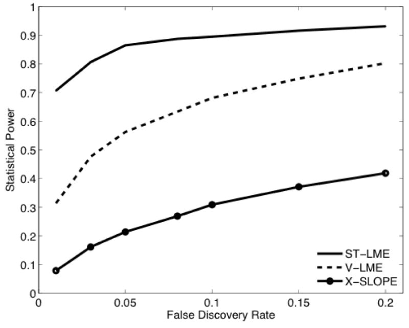
Empirical sensitivity (statistical power) as a function of FDR q-value on AD+HC sub-samples with 2N = 30, randomly drawn from the complete ADNI data (800 random sub-samples). Sensitivity is quantified as the fraction of instances, where the corresponding statistical method detected some group difference at a given FDR q-value. X-Slope: vertex-wise cross-subject analysis of cortical thinning rates estimated by fitting a line to serial measurements; V-LME: vertex-wise application of the LME approach to longitudinal thickness data; ST-LME: the proposed spatiotemporal LME modeling method applied to longitudinal thickness data.
Figure 2.

Statistical power as a function of sample size (2N) with FDR q-value = 0.05. See caption of Figure 1 for further details.
Figure 3.

Repeatability quantified as the agreement (area overlap) of the detected regions between two independent samples (400 independent AD+HC sample pairs of size 2N=30) as a function of FDR q-value. Error bars show standard error of the mean. See caption of Figure 1 for legend.
Figure 4.

Repeatability quantified as the agreement (area overlap) of the detected regions between two independent samples as a function of sample size (with FDR q-value = 0.05). See caption of Figure 3 for further details.
Finally, we conducted a sensitivity analysis of the ST-LME results to assess the effect of varying the segmentation parameter k. These results, presented in the Supplementary Material, reveal that the statistical power, repeatability and type I error control offered by ST-LME are influenced by the segmentation step, and in particular by the size and number of the segmentation regions. In general, as k is increased, the segmentation step outputs larger regions, which in turn can boost statistical power. However, when these regions are too big (e.g., when k = 2.5) ST-LME becomes prone to type I errors, because the model’s assumption that the temporal covariance structure is the same across the vertices in each region is likely to be violated. Thus, in general we recommend k to be set between 1 and 2.
3.2 Comparing rates of atrophy across four clinical groups
Now, we present the maps revealed by the ST-LME and X-Slope approaches for characterizing longitudinal thinning differences between four well-studied clinical groups (HC, stable MCI –sMCI-, converter MCI –cMCI-, and AD patients), using the entire ADNI dataset. The surface FWHM used for smoothing the thickness data for this analysis was 8 mm. In the Supplementary Material, we provide supporting evidence for the validity of the assumptions in the ST-LME approach based on this analysis.
Figures 5 and 6 show the maps for comparing the rates of cortical thinning between HC and AD subjects obtained using the two methods: ST-LME and X-Slope. Figures 7 and 8 show the same comparisons between sMCI and cMCI subjects. We make several important observations. First, the ST-LME maps of cortical thinning associated with clinical Alzheimer’s and conversion from MCI to AD are in strong agreement with prior findings (Dickerson et al., 2009; Singh et al., 2006). Second, ST-LME reveals a dramatically wider extent of significant cortical thinning compared to X-Slope for both the AD vs. HC and stable vs. converter MCI analyses. The difference is particularly striking for the MCI group analysis of Figures 7 and 8, where X-Slope was barely able to detect any significant longitudinal difference between stable and converter MCI subjects. Finally, the sMCI vs. cMCI map obtained with ST-LME is remarkably similar to the AD vs. HC map obtained with X-Slope. This is likely pointing to a statistical power issue. The regions exhibiting a large difference of cortical thinning in AD (and thus are detectable by X-Slope) probably exhibit a relatively smaller effect in the MCI group as well, which apparently is detectable by a powerful method such as ST-LME, but not by X-Slope. The decreased effect size in the MCI group could be due to either a smaller difference in atrophy rates, which would be consistent with cortical thinning accelerating throughout this phase, or the clinical heterogeneity in the MCI population, or both.
Figure 5.
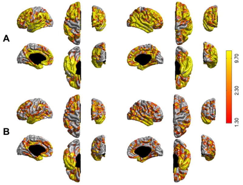
Uncorrected statistical significance –negative log10(p-value)- maps comparing longitudinal cortical thinning rates between HC (N=210) and AD (N=188) subjects (from the entire ADNI sample) visualized on the pial surface of the FreeSurfer template (fsaverage): (A) ST-LME method and (B) X-Slope method. The left hemisphere is shown on the left, and the right hemisphere is on the right. Vertices that have an uncorrected p-value less than 0.05 are shown in color. The odd-numbered rows show the lateral, superior, and anterior views. The even-numbered rows show the medial, inferior, and posterior views. Colorbar shows the corresponding significance value.
Figure 6.
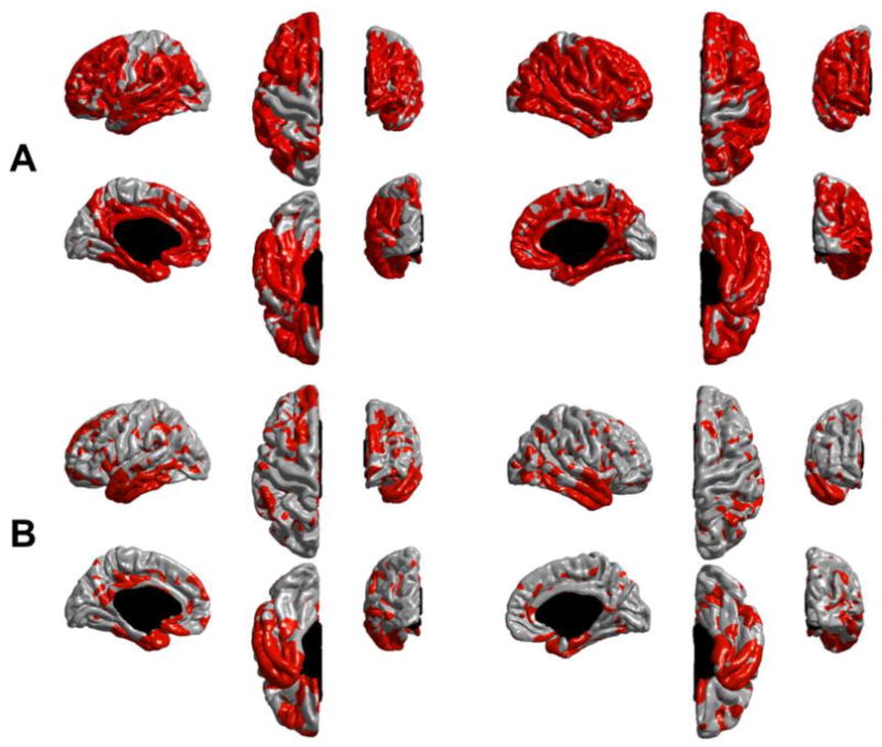
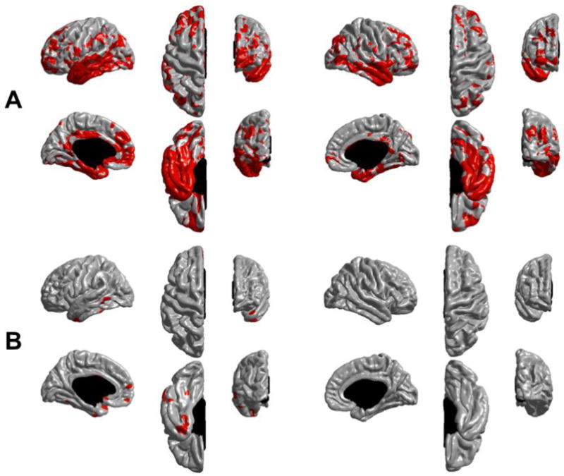
Cortical regions exhibiting a statistically significant difference in longitudinal thinning between HC and AD subjects (in red) on the entire ADNI sample. These maps were derived by thresholding the values shown in Figure 5 with an FDR correction at q=0.05. (A) ST-LME method and (B) X-Slope method. ST-LME reveals a much wider extent of significant thinning in AD.
Figure 7.
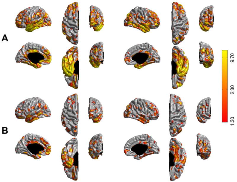
Uncorrected statistical significance –negative log10(p-value)- maps comparing longitudinal cortical thinning rates between stable MCI (N=227) and converter MCI (N=166) subjects (from the entire ADNI sample) visualized on the pial surface of the FreeSurfer template (fsaverage): (A) ST-LME method and (B) X-Slope method. See caption of Figure 5 for further details.
Figure 8.
Cortical regions exhibiting a statistically significant difference in longitudinal thinning between stable and converter MCI subjects (in red). These maps were derived by thresholding the values shown in Figure 7 with an FDR correction at q=0.05. (A) ST-LME method and (B) X-Slope method. ST-LME reveals a much more dramatic extent of significant thinning differences between two groups.
Finally, Supplementary Figure S9 shows the cortical thinning group comparison maps obtained with V-LME. These maps are almost identical to those obtained with ST-LME, suggesting that the two LME-based methods offer similar statistical power on the entire ADNI dataset, which contains over 750 subjects. This is in agreement with our previous results that indicated that the difference in the statistical power offered by V-LME and ST-LME decreases with increasing sample size.
3.3 Supplementary Experiments on the OASIS dataset
In the Supplementary Material, we provide further experiments that we conducted on the healthy subjects of the longitudinal OASIS dataset (Marcus et al., 2010; Marcus et al., 2007). In these experiments, we focused on healthy aging. Thus, instead of conducting a case-control group difference analysis, our effect of interest was simply nonzero longitudinal thinning across the cortex. Our results from the OASIS supplementary experiments are in full agreement with the ADNI experiments, and hence help us generalize our conclusions about the statistical power, repeatability and type I error control offered by ST-LME to applications other than dementia.
4 DISCUSSION
LME models provide a powerful and flexible approach for analyzing longitudinal data, while elegantly handling variable missing rates and non-uniform timing, and making use of subjects with a single time-point in order to characterize population-level variation (Bernal-Rusiel et al., 2012; Fitzmaurice et al., 2011). In this work, we extended the LME framework to exploit the spatial structure in neuroimage data and apply it to mass-univariate analysis. Our empirical results demonstrated that the proposed spatiotemporal LME (ST-LME) strategy offers significantly higher statistical power than a vertex-wise naïve application of LME and an alternative benchmark method commonly used in prior LNI studies. This boost in statistical power is particularly dramatic for studies with relatively modest sample size.
In our first experiment, we conducted a direct comparison of the statistical performance afforded by the proposed ST-LME approach and two benchmark methods, namely the vertex-wise application of the LME strategy (V-LME) and a vertex-wise cross-subject analysis of within-subject slope estimates (X-Slope), using the longitudinal ADNI data, which consisted of healthy controls (HC), subjects with MCI, and AD patients. We employed FreeSurfer’s tools to automatically compute thickness measurements across the entire cortical mantle of each subject, which were then normalized to a common template. By randomly sampling from the ADNI data, we created sub-groups of AD+HC (2N=20-50, 800 random samples, or 400 independent pairs of samples) and HC+HC (2N=20-50, 400 random samples) subjects.
Our analysis based on HC+HC samples, where no group differences were expected, revealed that all three methods provided a conservative control of specificity- well within the bounds predicted by theory. Next, we assessed sensitivity and repeatability on AD+HC samples of varying size (N=10-25). This analysis exposed the dramatic gain in statistical power offered by the proposed ST-LME approach, especially when the sample size was modest. At a typical FDR q-value of 0.05 and with N = 15, ST-LME afforded an empirical true positive rate (quantified at the sample level) of 0.87, whereas V-LME and X-Slope’s sensitivity were approximately 0.56 and 0.21, which represents a 55% and 314% gain, respectively. Our results further revealed that the difference in the statistical power offered by ST-LME and V-LME decreased as the sample size increased.
As expected, this increased sensitivity translated into a remarkable increase in the reliability of discoveries (see Figures 3-4). The average overlap area between the detected regions in two independent AD+HC samples of N=15 at FDR q=0.05 was 0 mm2 for X-Slope, 236 mm2 for V-LME and 1456 mm2 for ST-LME. We emphasize that the ST-LME results were generated by running the segmentation step separately for each new sample. Thus, the reported empirical repeatability measures also reflect the variation in the segmentation step.
We further quantified the effect of the segmentation step by running the same ST-LME analyses for different settings of the segmentation parameter k. These supplementary experiments demonstrated that the proposed ST-LME method offers increased statistical power and repeatability over V-LME for the recommended range of k values between 1 and 2, while providing good control of type I error. In general with higher k values, the segmentation step produced larger regions, which improved efficiency but increased the type I error. Our experiments suggested that for a wide range of k values (k<= 2), the type I error was successfully controlled with the employed FDR procedure.
In our second set of experiments, we conducted mass-univariate analyses of cortical thinning on the entire ADNI data. Our results, which were in strong agreement with the literature, illustrated the use of the proposed ST-LME strategy in mapping disease-specific longitudinal thinning effects. They further highlighted the dramatic gain in statistical power offered by V-LME and ST-LME compared to X-Slope. The cortical thinning maps obtained by the LME methods revealed a substantially larger extent of cortical thinning associated with AD and MCI to AD conversion. There was little difference between the maps of V-LME (presented in the Supplementary Material) and ST-LME, probably because the sample size of this experiment was relatively large and the study was well powered.
Finally, we conducted additional experiments on a different dataset (OASIS), where the effect of interest was aging-associated atrophy and not dementia-related. Our results, in general, confirmed our ADNI observations: ST-LME offers a substantial boost in statistical efficiency, while maintaining good control of type I error rates.
The proposed ST-LME approach exploits the inherent spatial structure in neuroimaging data by treating subsets of locations as having the same temporal covariance structure, as suggested by (Friston et al., 2005), and modeling the local spatial correlations in the data (Bowman, 2007). To achieve this, the entire image is adaptively segmented into relatively small homogeneous regions of variable sizes and a region-wise spatiotemporal model is constructed via a Kronecker tensor product between a parametric spatial correlation matrix and the classical mixed effects temporal covariance matrix. This resulted in parsimonious yet effective models for the spatiotemporal covariances within homogeneous regions.
To our knowledge, there are only two other recently published methods that are focused on mass-univariate longitudinal image analysis (Li et al., 2013; Skup et al., 2012). These methods utilize a marginal modeling approach (such as generalized estimating equations, GEE, and its variants), which provides a complementary strategy to the LME methods we employed in our own work. In contrast with the generalized linear model setting, in the linear model setting, LME and GEE-type methods can lead to very similar types of inferences (Fitzmaurice et al., 2011), although there are subtle, yet important distinctions between the two approaches. The major advantages offered by the LME approach are that it enables the explicit modeling and analysis of within and across-subject sources of variability in the temporal covariance, can elegantly handle unbalanced data, and most importantly provides a valid inference strategy for the small-sample setting, which is common in neuroimaging studies. Crucially, inference in GEE-type methods relies on asymptotic distributions, which might not be appropriate for studies where N is small. We refer the reader to (Fitzmaurice et al., 2011) for a detailed discussion of this issue.
We plan to further investigate several open issues in the future. The segmentation algorithm we used in the present work might be sub-optimal and a better strategy would be to incorporate the spatial correlation model into the segmentation step. That said, our empirical results suggest that even with the employed sub-optimal segmentation step, the proposed ST-LME approach provides increased statistical efficiency. There are also alternative strategies we would like to examine for modeling/exploiting the spatial smoothness of image data. One such method is the recently proposed MARM framework (Li et al., 2011), which has the advantage of being adaptive and multi-scale.
The hypothesis testing strategy we used in our work employed a 50:50 mixture of chi-square distributions, as suggested in (Fitzmaurice et al., 2011). There is a recent debate on whether this is an optimal strategy, or whether better approximate distributions exist, cf. (Greven et al., 2008). Future work will further examine this issue in more detail and consider alternative inference methods in the context of neuroimage analysis.
Other directions we plan to explore include using surface-based distances between vertices to improve the accuracy of the spatial covariance parameterization and employing alternative multiple comparisons correction methods, for example those based on the topology of the statistical maps, which might provide a further statistical boost in examining longitudinal effects.
5 CONCLUSIONS
We presented a spatial extension of the linear mixed effects (LME) approach, which provides a powerful and flexible framework for the mass-univariate analysis of longitudinal neuroimage data. We have implemented and validated these tools for mapping longitudinal cortical thinning effects within the FreeSurfer framework. The proposed approach is general and can be adapted to the analysis of any type of longitudinal spatial data.
Supplementary Material
HIGHLIGHTS.
We apply Linear Mixed Effects (LME) models to longitudinal imaging
We develop a spatial extension of LME for mass-univariate analysis
We illustrate, validate and benchmark the proposed method
These tools will be freely available in FreeSurfer
Footnotes
A noteworthy exception is AFNI (Cox, R.W., 1996. AFNI: software for analysis and visualization of functional magnetic resonance neuroimages. Computers and Biomedical Research 29, 162-173.), a functional MRI analysis toolkit, which provides LME-based tools.
Random effects typically include an intercept and/or time-varying variables.
By homogeneous, we mean the covariance structure of subject-level serial measurements within each region can be considered to have a similar temporal component and a relatively smooth spatial component. We note that we are not assuming that the effect of interest is homogeneous within each region. As we discuss below the effect of interest is not used to obtain the segmentation, thus we avoid the issue of “double-dipping.” I.e., the proposed two-step strategy (segmentation + model fitting/hypothesis testing) is not coupled in a way that would bias the statistical results.
As we show in the following section, there are closed-form formulae for the OLS parameter estimates and the residuals can thus be computed efficiently.
Although this issue can incidentally be addressed with more appropriate methods like weigthed least squares, we are not aware of any prior neuroimaging study that does this.
Publisher's Disclaimer: This is a PDF file of an unedited manuscript that has been accepted for publication. As a service to our customers we are providing this early version of the manuscript. The manuscript will undergo copyediting, typesetting, and review of the resulting proof before it is published in its final citable form. Please note that during the production process errors maybe discovered which could affect the content, and all legal disclaimers that apply to the journal pertain.
References
- Asami T, Bouix S, Whitford TJ, Shenton ME, Salisbury DF, McCarley RW. Longitudinal loss of gray matter volume in patients with first-episode schizophrenia: DARTEL automated analysis and ROI validation. Neuroimage. 2011 doi: 10.1016/j.neuroimage.2011.08.066. [DOI] [PMC free article] [PubMed] [Google Scholar]
- Benjamini Y, Krieger AM, Yekutieli D. Adaptive linear step-up procedures that control the false discovery rate. Biometrika. 2006;93:491–507. [Google Scholar]
- Bernal-Rusiel JL, Atienza M, Cantero JL. Determining the optimal level of smoothing in cortical thickness analysis: A hierarchical approach based on sequential statistical thresholding. Neuroimage. 2010;52:158–171. doi: 10.1016/j.neuroimage.2010.03.074. [DOI] [PubMed] [Google Scholar]
- Bernal-Rusiel JL, Greve DN, Reuter M, Fischl B, Sabuncu MR. Statistical analysis of longitudinal neuroimage data with Linear Mixed Effects models. Neuroimage. 2012:249–260. doi: 10.1016/j.neuroimage.2012.10.065. [DOI] [PMC free article] [PubMed] [Google Scholar]
- Blockx I, Van Camp N, Verhoye M, Boisgard R, Dubois A, Jego B, Jonckers E, Raber K, Siquier K, Kuhnast B, Dolle F, Nguyen HP, Von Horsten S, Tavitian B, Van der Linden A. Genotype specific age related changes in a transgenic rat model of Huntington’s disease. Neuroimage. 2011;58:1006–1016. doi: 10.1016/j.neuroimage.2011.07.007. [DOI] [PubMed] [Google Scholar]
- Bowman FD. Spatiotemporal models for region of interest analyses of functional neuroimaging data. Journal of the American Statistical Association. 2007;102:442–453. [Google Scholar]
- Bowman FD, Caffo BS, Spear Bassett S, Kilts C. A Bayesian hierarchical framework for spatial modeling of fMRI data. 2008 doi: 10.1016/j.neuroimage.2007.08.012. [DOI] [PMC free article] [PubMed] [Google Scholar]
- Bowman FD, Kilts C. Modeling intra-subject correlation among repeated scans in positron emission tomography (PET) neuroimaging data. Human brain mapping. 2003;20:59–70. doi: 10.1002/hbm.10127. [DOI] [PMC free article] [PubMed] [Google Scholar]
- Chetelat G, Landeau B, Eustache F, Mezenge F, Viader F, de La Sayette V, Desgranges B, Baron JC. Using voxel-based morphometry to map the structural changes associated with rapid conversion in MCI: a longitudinal MRI study. Neuroimage. 2005;27:934–946. doi: 10.1016/j.neuroimage.2005.05.015. [DOI] [PubMed] [Google Scholar]
- Cox RW. AFNI: software for analysis and visualization of functional magnetic resonance neuroimages. Computers and Biomedical Research. 1996;29:162–173. doi: 10.1006/cbmr.1996.0014. [DOI] [PubMed] [Google Scholar]
- Davatzikos C, Resnick SM. Degenerative age changes in white matter connectivity visualized in vivo using magnetic resonance imaging. Cerebral cortex. 2002;12:767–771. doi: 10.1093/cercor/12.7.767. [DOI] [PubMed] [Google Scholar]
- Delaloye C, Moy G, de Bilbao F, Weber K, Baudois S, Haller S, Xekardaki A, Canuto A, Giardini U, Lövblad KO. Longitudinal analysis of cognitive performances and structural brain changes in late- life bipolar disorder. International journal of geriatric psychiatry. 2011;26:1309–1318. doi: 10.1002/gps.2683. [DOI] [PubMed] [Google Scholar]
- Derado G, Bowman FD, Zhang L. Predicting brain activity using a Bayesian spatial model. Statistical Methods in Medical Research. 2012 doi: 10.1177/0962280212448972. [DOI] [PMC free article] [PubMed] [Google Scholar]
- Desikan RS, McEvoy LK, Thompson WK, Holland D, Roddey JC, Blennow K, Aisen PS, Brewer JB, Hyman BT, Dale AM. Amyloid- β associated volume loss occurs only in the presence of phospho- tau. Annals of neurology. 2011 doi: 10.1002/ana.22509. [DOI] [PMC free article] [PubMed] [Google Scholar]
- Dickerson BC, Bakkour A, Salat DH, Feczko E, Pacheco J, Greve DN, Grodstein F, Wright CI, Blacker D, Rosas HD. The cortical signature of Alzheimer’s disease: regionally specific cortical thinning relates to symptom severity in very mild to mild AD dementia and is detectable in asymptomatic amyloid-positive individuals. Cerebral cortex. 2009;19:497–510. doi: 10.1093/cercor/bhn113. [DOI] [PMC free article] [PubMed] [Google Scholar]
- Draganski B, Gaser C, Busch V, Schuierer G, Bogdahn U, May A. Neuroplasticity: changes in grey matter induced by training. Nature. 2004;427:311–312. doi: 10.1038/427311a. [DOI] [PubMed] [Google Scholar]
- Driscoll I, Beydoun MA, An Y, Davatzikos C, Ferrucci L, Zonderman AB, Resnick SM. Midlife obesity and trajectories of brain volume changes in older adults. Human brain mapping. 2011 doi: 10.1002/hbm.21353. [DOI] [PMC free article] [PubMed] [Google Scholar]
- Fischl B. Freesurfer. Neuroimage. 2012 doi: 10.1016/j.neuroimage.2012.01.021. [DOI] [PMC free article] [PubMed] [Google Scholar]
- Fischl B, Dale AM. Measuring the thickness of the human cerebral cortex from magnetic resonance images. Proceedings of the National Academy of Sciences. 2000;97:11050. doi: 10.1073/pnas.200033797. [DOI] [PMC free article] [PubMed] [Google Scholar]
- Fischl B, Sereno MI, Dale AM. Cortical Surface-Based Analysis* 1:: II: Inflation, Flattening, and a Surface-Based Coordinate System. Neuroimage. 1999a;9:195–207. doi: 10.1006/nimg.1998.0396. [DOI] [PubMed] [Google Scholar]
- Fischl B, Sereno MI, Tootell RBH, Dale AM. High-resolution intersubject averaging and a coordinate system for the cortical surface. Human brain mapping. 1999b;8:272–284. doi: 10.1002/(SICI)1097-0193(1999)8:4<272::AID-HBM10>3.0.CO;2-4. [DOI] [PMC free article] [PubMed] [Google Scholar]
- Fitzmaurice GM, Laird NM, Ware JH. Applied longitudinal analysis. Wiley; 2011. [Google Scholar]
- Fjell AM, Walhovd KB, Fennema-Notestine C, McEvoy LK, Hagler DJ, Holland D, Brewer JB, Dale AM. One-year brain atrophy evident in healthy aging. The Journal of Neuroscience. 2009;29:15223–15231. doi: 10.1523/JNEUROSCI.3252-09.2009. [DOI] [PMC free article] [PubMed] [Google Scholar]
- Fotenos AF, Snyder A, Girton L, Morris J, Buckner R. Normative estimates of cross-sectional and longitudinal brain volume decline in aging and AD. Neurology. 2005;64:1032–1039. doi: 10.1212/01.WNL.0000154530.72969.11. [DOI] [PubMed] [Google Scholar]
- Fouquet M, Desgranges B, Landeau B, Duchesnay E, Mézenge F, De La Sayette V, Viader F, Baron JC, Eustache F, Chételat G. Longitudinal brain metabolic changes from amnestic mild cognitive impairment to Alzheimer’s disease. Brain. 2009;132:2058–2067. doi: 10.1093/brain/awp132. [DOI] [PMC free article] [PubMed] [Google Scholar]
- Frings L, Mader I, Landwehrmeyer BG, Weiller C, Hüll M, Huppertz HJ. Quantifying change in individual subjects affected by frontotemporal lobar degeneration using automated longitudinal MRI volumetry. Human brain mapping. 2011 doi: 10.1002/hbm.21304. [DOI] [PMC free article] [PubMed] [Google Scholar]
- Friston K, Stephan K, Lund T, Morcom A, Kiebel S. Mixed-effects and fMRI studies. Neuroimage. 2005;24:244–252. doi: 10.1016/j.neuroimage.2004.08.055. [DOI] [PubMed] [Google Scholar]
- Friston KJ. Statistical parametric mapping: the analysis of functional brain images. Academic Press; 2007. [Google Scholar]
- Friston KJ, Glaser DE, Henson RN, Kiebel S, Phillips C, Ashburner J. Classical and Bayesian inference in neuroimaging: applications. Neuroimage. 2002a;16:484–512. doi: 10.1006/nimg.2002.1091. [DOI] [PubMed] [Google Scholar]
- Friston KJ, Penny W, Phillips C, Kiebel S, Hinton G, Ashburner J. Classical and Bayesian inference in neuroimaging: theory. Neuroimage. 2002b;16:465–483. doi: 10.1006/nimg.2002.1090. [DOI] [PubMed] [Google Scholar]
- Giedd JN, Blumenthal J, Jeffries NO, Castellanos FX, Liu H, Zijdenbos A, Paus T, Evans AC, Rapoport JL. Brain development during childhood and adolescence: a longitudinal MRI study. Nature neuroscience. 1999;2:861–862. doi: 10.1038/13158. [DOI] [PubMed] [Google Scholar]
- Gonzales R, Woods RE, Eddins S. Digital Image Processing. Prentice Hall; New Jersey: 2002. [Google Scholar]
- Gossl C, Auer DP, Fahrmeir L. Bayesian spatiotemporal inference in functional magnetic resonance imaging. Biometrics. 2004;57:554–562. doi: 10.1111/j.0006-341x.2001.00554.x. [DOI] [PubMed] [Google Scholar]
- Greven S, Crainiceanu CM, K…ºchenhoff H, Peters A. Restricted likelihood ratio testing for zero variance components in linear mixed models. Journal of Computational and Graphical Statistics. 2008;17 [Google Scholar]
- Guo Y, DuBois Bowman F, Kilts C. Predicting the brain response to treatment using a Bayesian hierarchical model with application to a study of schizophrenia. Human brain mapping. 2008;29:1092–1109. doi: 10.1002/hbm.20450. [DOI] [PMC free article] [PubMed] [Google Scholar]
- Han X, Jovicich J, Salat D, van der Kouwe A, Quinn B, Czanner S, Busa E, Pacheco J, Albert M, Killiany R. Reliability of MRI-derived measurements of human cerebral cortical thickness: the effects of field strength, scanner upgrade and manufacturer. Neuroimage. 2006;32:180–194. doi: 10.1016/j.neuroimage.2006.02.051. [DOI] [PubMed] [Google Scholar]
- Hedman AM, van Haren NEM, Schnack HG, Kahn RS, Hulshoff Pol HE. Human brain changes across the life span: A review of 56 longitudinal magnetic resonance imaging studies. Human brain mapping. 2011 doi: 10.1002/hbm.21334. [DOI] [PMC free article] [PubMed] [Google Scholar]
- Ho BC, Andreasen NC, Nopoulos P, Arndt S, Magnotta V, Flaum M. Progressive structural brain abnormalities and their relationship to clinical outcome: a longitudinal magnetic resonance imaging study early in schizophrenia. Archives of General Psychiatry. 2003;60:585. doi: 10.1001/archpsyc.60.6.585. [DOI] [PubMed] [Google Scholar]
- Holland D, Brewer JB, Hagler DJ, Fennema-Notestine C, Dale AM, Weiner M, Thal L, Petersen R, Jack CR, Jr, Jagust W. Subregional neuroanatomical change as a biomarker for Alzheimer’s disease. Proceedings of the National Academy of Sciences. 2009;106:20954–20959. doi: 10.1073/pnas.0906053106. [DOI] [PMC free article] [PubMed] [Google Scholar]
- Holland D, McEvoy LK, Dale AM. Unbiased comparison of sample size estimates from longitudinal structural measures in ADNI. Human brain mapping. 2011 doi: 10.1002/hbm.21386. [DOI] [PMC free article] [PubMed] [Google Scholar]
- Hua X, Hibar DP, Lee S, Toga AW, Jack CR, Jr, Weiner MW, Thompson PM. Sex and age differences in atrophic rates: an ADNI study with n= 1368 MRI scans. Neurobiology of aging. 2010;31:1463–1480. doi: 10.1016/j.neurobiolaging.2010.04.033. [DOI] [PMC free article] [PubMed] [Google Scholar]
- Hua X, Leow AD, Levitt JG, Caplan R, Thompson PM, Toga AW. Detecting brain growth patterns in normal children using tensor- based morphometry. Human brain mapping. 2009;30:209–219. doi: 10.1002/hbm.20498. [DOI] [PMC free article] [PubMed] [Google Scholar]
- Jack CR, Jr, Lowe VJ, Weigand SD, Wiste HJ, Senjem ML, Knopman DS, Shiung MM, Gunter JL, Boeve BF, Kemp BJ. Serial PIB and MRI in normal, mild cognitive impairment and Alzheimer’s disease: implications for sequence of pathological events in Alzheimer’s disease. Brain. 2009;132:1355–1365. doi: 10.1093/brain/awp062. [DOI] [PMC free article] [PubMed] [Google Scholar]
- Jack CR, Jr, Weigand SD, Shiung MM, Przybelski SA, O’Brien PC, Gunter JL, Knopman DS, Boeve BF, Smith GE, Petersen RC. Atrophy rates accelerate in amnestic mild cognitive impairment. Neurology. 2008;70:1740–1752. doi: 10.1212/01.wnl.0000281688.77598.35. [DOI] [PMC free article] [PubMed] [Google Scholar]
- Josephs KA, Whitwell JL, Ahmed Z, Shiung MM, Weigand SD, Knopman DS, Boeve BF, Parisi JE, Petersen RC, Dickson DW. β- amyloid burden is not associated with rates of brain atrophy. Annals of neurology. 2008;63:204–212. doi: 10.1002/ana.21223. [DOI] [PMC free article] [PubMed] [Google Scholar]
- Kaladjian A, Jeanningros R, Azorin JM, Nazarian B, Roth M, Anton JL, Mazzola- Pomietto P. Remission from mania is associated with a decrease in amygdala activation during motor response inhibition. Bipolar disorders. 2009;11:530–538. doi: 10.1111/j.1399-5618.2009.00722.x. [DOI] [PubMed] [Google Scholar]
- Kalkers NF, Ameziane N, Bot JCJ, Minneboo A, Polman CH, Barkhof F. Longitudinal brain volume measurement in multiple sclerosis: rate of brain atrophy is independent of the disease subtype. Archives of Neurology. 2002;59:1572. doi: 10.1001/archneur.59.10.1572. [DOI] [PubMed] [Google Scholar]
- Kasai K, Shenton ME, Salisbury DF, Hirayasu Y, Onitsuka T, Spencer MH, Yurgelun-Todd DA, Kikinis R, Jolesz FA, McCarley RW. Progressive decrease of left Heschl gyrus and planum temporale gray matter volume in first-episode schizophrenia: a longitudinal magnetic resonance imaging study. Archives of General Psychiatry. 2003;60:766. doi: 10.1001/archpsyc.60.8.766. [DOI] [PMC free article] [PubMed] [Google Scholar]
- Kenward MG, Roger JH. Small sample inference for fixed effects from restricted maximum likelihood. Biometrics. 1997:983–997. [PubMed] [Google Scholar]
- Laird N, Lange N, Stram D. Maximum likelihood computations with repeated measures: application of the EM algorithm. Journal of the American Statistical Association. 1987:97–105. [Google Scholar]
- Lau JC, Lerch JP, Sled JG, Henkelman RM, Evans AC, Bedell BJ. Longitudinal neuroanatomical changes determined by deformation-based morphometry in a mouse model of Alzheimer’s disease. Neuroimage. 2008;42:19–27. doi: 10.1016/j.neuroimage.2008.04.252. [DOI] [PubMed] [Google Scholar]
- Lerch JP, Pruessner JC, Zijdenbos A, Hampel H, Teipel SJ, Evans AC. Focal decline of cortical thickness in Alzheimer’s disease identified by computational neuroanatomy. Cereb Cortex. 2005;15:995–1001. doi: 10.1093/cercor/bhh200. [DOI] [PubMed] [Google Scholar]
- Li Y, Gilmore JH, Shen D, Styner M, Lin W, Zhu H. Multiscale Adaptive Generalized Estimating Equations for Longitudinal Neuroimaging Data. Neuroimage. 2013 doi: 10.1016/j.neuroimage.2013.01.034. [DOI] [PMC free article] [PubMed] [Google Scholar]
- Li Y, Zhu H, Shen D, Lin W, Gilmore JH, Ibrahim JG. Multiscale adaptive regression models for neuroimaging data. Journal of the Royal Statistical Society: Series B (Statistical Methodology) 2011;73:559–578. doi: 10.1111/j.1467-9868.2010.00767.x. [DOI] [PMC free article] [PubMed] [Google Scholar]
- Marcus DS, Fotenos AF, Csernansky JG, Morris JC, Buckner RL. Open access series of imaging studies: longitudinal MRI data in nondemented and demented older adults. Journal of cognitive neuroscience. 2010;22:2677–2684. doi: 10.1162/jocn.2009.21407. [DOI] [PMC free article] [PubMed] [Google Scholar]
- Marcus DS, Wang TH, Parker J, Csernansky JG, Morris JC, Buckner RL. Open Access Series of Imaging Studies (OASIS): cross-sectional MRI data in young, middle aged, nondemented, and demented older adults. Journal of cognitive neuroscience. 2007;19:1498–1507. doi: 10.1162/jocn.2007.19.9.1498. [DOI] [PubMed] [Google Scholar]
- Martensson J, Eriksson J, Bodammer NC, Lindgren M, Johansson M, Nyberg L, Lovden M. Growth of language-related brain areas after foreign language learning. Neuroimage. 2012 doi: 10.1016/j.neuroimage.2012.06.043. [DOI] [PubMed] [Google Scholar]
- Ment LR, Kesler S, Vohr B, Katz KH, Baumgartner H, Schneider KC, Delancy S, Silbereis J, Duncan CC, Constable RT. Longitudinal brain volume changes in preterm and term control subjects during late childhood and adolescence. Pediatrics. 2009;123:503–511. doi: 10.1542/peds.2008-0025. [DOI] [PMC free article] [PubMed] [Google Scholar]
- Misra C, Fan Y, Davatzikos C. Baseline and longitudinal patterns of brain atrophy in MCI patients, and their use in prediction of short-term conversion to AD: results from ADNI. Neuroimage. 2009;44:1415. doi: 10.1016/j.neuroimage.2008.10.031. [DOI] [PMC free article] [PubMed] [Google Scholar]
- Pantelis C, Velakoulis D, McGorry PD, Wood SJ, Suckling J, Phillips LJ, Yung AR, Bullmore ET, Brewer W, Soulsby B. Neuroanatomical abnormalities before and after onset of psychosis: a cross-sectional and longitudinal MRI comparison. The Lancet. 2003;361:281–288. doi: 10.1016/S0140-6736(03)12323-9. [DOI] [PubMed] [Google Scholar]
- Paviour DC, Price SL, Jahanshahi M, Lees AJ, Fox NC. Longitudinal MRI in progressive supranuclear palsy and multiple system atrophy: rates and regions of atrophy. Brain. 2006;129:1040–1049. doi: 10.1093/brain/awl021. [DOI] [PubMed] [Google Scholar]
- Resnick S, Sojkova J, Zhou Y, An Y, Ye W, Holt D, Dannals R, Mathis C, Klunk W, Ferrucci L. Longitudinal cognitive decline is associated with fibrillar amyloid-beta measured by [11C] PiB. Neurology. 2010;74:807–815. doi: 10.1212/WNL.0b013e3181d3e3e9. [DOI] [PMC free article] [PubMed] [Google Scholar]
- Reuter M, Fischl B. Avoiding asymmetry-induced bias in longitudinal image processing. Neuroimage. 2011;57:19–21. doi: 10.1016/j.neuroimage.2011.02.076. [DOI] [PMC free article] [PubMed] [Google Scholar]
- Reuter M, Rosas HD, Fischl B. Highly accurate inverse consistent registration: A robust approach. Neuroimage. 2010;53:1181–1196. doi: 10.1016/j.neuroimage.2010.07.020. [DOI] [PMC free article] [PubMed] [Google Scholar]
- Reuter M, Schmansky NJ, Rosas HD, Fischl B. Within-subject template estimation for unbiased longitudinal image analysis. Neuroimage . 2012 doi: 10.1016/j.neuroimage.2012.02.084. http://dx.doi.org/10.1016/j.neuroimage.2012.02.084. [DOI] [PMC free article] [PubMed]
- Rosas HD, Reuter M, Doros G, Lee SY, Triggs T, Malarick K, Fischl B, Salat DH, Hersch SM. A tale of two factors: What determines the rate of progression in Huntington’s disease? A longitudinal MRI study. Movement Disorders. 2011;26:1691–1697. doi: 10.1002/mds.23762. [DOI] [PMC free article] [PubMed] [Google Scholar]
- Sabuncu MR, Desikan RS, Sepulcre J, Yeo BTT, Liu H, Schmansky NJ, Reuter M, Weiner MW, Buckner RL, Sperling RA. The dynamics of cortical and hippocampal atrophy in Alzheimer disease. Archives of Neurology. 2011;68:1040. doi: 10.1001/archneurol.2011.167. [DOI] [PMC free article] [PubMed] [Google Scholar]
- Schuff N, Tosun D, Insel PS, Chiang GC, Truran D, Aisen PS, Jack CR, Jr, Weiner MW. Nonlinear time course of brain volume loss in cognitively normal and impaired elders. Neurobiology of aging. 2010 doi: 10.1016/j.neurobiolaging.2010.07.012. [DOI] [PMC free article] [PubMed] [Google Scholar]
- Schumann CM, Bloss CS, Barnes CC, Wideman GM, Carper RA, Akshoomoff N, Pierce K, Hagler D, Schork N, Lord C. Longitudinal magnetic resonance imaging study of cortical development through early childhood in autism. The Journal of Neuroscience. 2010;30:4419–4427. doi: 10.1523/JNEUROSCI.5714-09.2010. [DOI] [PMC free article] [PubMed] [Google Scholar]
- Shaw P, Kabani NJ, Lerch JP, Eckstrand K, Lenroot R, Gogtay N, Greenstein D, Clasen L, Evans A, Rapoport JL. Neurodevelopmental trajectories of the human cerebral cortex. The Journal of Neuroscience. 2008;28:3586–3594. doi: 10.1523/JNEUROSCI.5309-07.2008. [DOI] [PMC free article] [PubMed] [Google Scholar]
- Shinohara RT, Crainiceanu CM, Caffo BS, Reich DS. Longitudinal analysis of spatiotemporal processes: a case study of dynamic contrast-enhanced magnetic resonance imaging in multiple sclerosis 2011 [Google Scholar]
- Sidtis JJ, Strother SC, Naoum A, Rottenberg DA, Gomez C. Longitudinal cerebral blood flow changes during speech in hereditary ataxia. Brain and language. 2010;114:43–51. doi: 10.1016/j.bandl.2010.03.007. [DOI] [PMC free article] [PubMed] [Google Scholar]
- Singh V, Chertkow H, Lerch JP, Evans AC, Dorr AE, Kabani NJ. Spatial patterns of cortical thinning in mild cognitive impairment and Alzheimer’s disease. Brain. 2006;129:2885–2893. doi: 10.1093/brain/awl256. [DOI] [PubMed] [Google Scholar]
- Skup M, Zhu H, Zhang H. Multiscale Adaptive Marginal Analysis of Longitudinal Neuroimaging Data with Time-Varying Covariates. Biometrics. 2012;68:1083–1092. doi: 10.1111/j.1541-0420.2012.01767.x. [DOI] [PMC free article] [PubMed] [Google Scholar]
- Sluimer JD, Van Der Flier WM, Karas GB, Fox NC, Scheltens P, Barkhof F, Vrenken H. Whole-Brain Atrophy Rate and Cognitive Decline: Longitudinal MR Study of Memory Clinic Patients1. Radiology. 2008;248:590–598. doi: 10.1148/radiol.2482070938. [DOI] [PubMed] [Google Scholar]
- Sluimer JD, Van Der Flier WM, Karas GB, Van Schijndel R, Barnes J, Boyes RG, Cover KS, Olabarriaga SD, Fox NC, Scheltens P. Accelerating regional atrophy rates in the progression from normal aging to Alzheimer’s disease. European radiology. 2009;19:2826–2833. doi: 10.1007/s00330-009-1512-5. [DOI] [PMC free article] [PubMed] [Google Scholar]
- Smith SM, Jenkinson M, Woolrich MW, Beckmann CF, Behrens TEJ, Johansen-Berg H, Bannister PR, De Luca M, Drobnjak I, Flitney DE. Advances in functional and structural MR image analysis and implementation as FSL. Neuroimage. 2004;23:S208–S219. doi: 10.1016/j.neuroimage.2004.07.051. [DOI] [PubMed] [Google Scholar]
- SPM. http://www.fil.ion.ucl.ac.uk/spm/
- Sullivan EV, Pfefferbaum A, Rohlfing T, Baker FC, Padilla ML, Colrain IM. Developmental change in regional brain structure over 7 months in early adolescence: Comparison of approaches for longitudinal atlas-based parcellation. Neuroimage. 2011 doi: 10.1016/j.neuroimage.2011.04.003. [DOI] [PMC free article] [PubMed] [Google Scholar]
- Thambisetty M, An Y, Kinsey A, Koka D, Saleem M, Kraut M, Ferrucci L. Plasma clusterin concentration is associated with longitudinal brain atrophy in mild cognitive impairment. Neuroimage. 2011 doi: 10.1016/j.neuroimage.2011.07.056. [DOI] [PMC free article] [PubMed] [Google Scholar]
- Thambisetty M, Wan J, Carass A, An Y, Prince JL, Resnick SM. Longitudinal changes in cortical thickness associated with normal aging. Neuroimage. 2010;52:1215–1223. doi: 10.1016/j.neuroimage.2010.04.258. [DOI] [PMC free article] [PubMed] [Google Scholar]
- Thirion B, Pinel P, M…©riaux S, Roche A, Dehaene S, Poline JB. Analysis of a large fMRI cohort: Statistical and methodological issues for group analyses. Neuroimage. 2007;35:105–120. doi: 10.1016/j.neuroimage.2006.11.054. [DOI] [PubMed] [Google Scholar]
- Verbeke G, Molenberghs G. Linear mixed models for longitudinal data. N.Y.: Springer; 2000. [Google Scholar]
- Wenger E, Schaefer S, Noack H, K…ºhn S, M…•rtensson J, Heinze HJ, D…ºzel E, B…§ckman L, Lindenberger U, L…∂vd…©n M. Cortical thickness changes following spatial navigation training in adulthood and aging. Neuroimage. 2011 doi: 10.1016/j.neuroimage.2011.11.015. [DOI] [PubMed] [Google Scholar]
- Whitwell J, Weigand S, Gunter J, Boeve B, Rademakers R, Baker M, Knopman D, Wszolek Z, Petersen R, Jack C., Jr Trajectories of brain and hippocampal atrophy in FTD with mutations in MAPT or GRN. Neurology. 2011;77:393–398. doi: 10.1212/WNL.0b013e318227047f. [DOI] [PMC free article] [PubMed] [Google Scholar]
- Whitwell JL, Jack CR, Jr, Parisi JE, Knopman DS, Boeve BF, Petersen RC, Ferman TJ, Dickson DW, Josephs KA. Rates of cerebral atrophy differ in different degenerative pathologies. Brain. 2007;130:1148–1158. doi: 10.1093/brain/awm021. [DOI] [PMC free article] [PubMed] [Google Scholar]
- Wilde EA, Merkley TL, Bigler ED, Max JE, Schmidt AT, Ayoub KW, McCauley SR, Hunter JV, Hanten G, Li X. Longitudinal changes in cortical thickness in children after traumatic brain injury and their relation to behavioral regulation and emotional control. International Journal of Developmental Neuroscience. 2012 doi: 10.1016/j.ijdevneu.2012.01.003. [DOI] [PMC free article] [PubMed] [Google Scholar]
- Woolrich MW, Jenkinson M, Brady JM, Smith SM. Fully Bayesian spatio-temporal modeling of fMRI data. Medical Imaging, IEEE Transactions. 2004;23:213–231. doi: 10.1109/TMI.2003.823065. on. [DOI] [PubMed] [Google Scholar]
- Zhang X, Johnson T, Little R, Cao Y. Longitudinal image analysis of tumor/brain change in contrast uptake induced by radiation. The University of Michigan Department of Biostatistics Working Paper Series. 2009 doi: 10.1111/j.1467-9876.2010.00718.x. [DOI] [PMC free article] [PubMed] [Google Scholar]
- Zipunnikov V, Greven S, Caffo B, Reich DS, Crainiceanu C. Longitudinal high-dimensional data analysis. 2011 doi: 10.1214/14-aoas748. [DOI] [PMC free article] [PubMed] [Google Scholar]
Associated Data
This section collects any data citations, data availability statements, or supplementary materials included in this article.