Unified Geometry and Topology Correction for Cortical Surface Reconstruction with Intrinsic Reeb Analysis

Abstract

A key challenge in the accurate reconstruction of cortical surfaces is the automated correction of geometric and topological outliers in tissue boundaries. Conventionally these two types of errors are handled separately. In this work, we propose a unified analysis framework for the joint correction of geometric and topological outliers in cortical reconstruction. Using the Reeb graph of intrinsically defined Laplace-Beltrami eigenfunctions, our method automatically locates spurious branches, handles and holes on tissue boundaries and corrects them with image information and geometric regularity derived from paired boundary evolutions. In our experiments, we demonstrate on 200 MR images from two datasets that our method is much faster and achieves better performance than FreeSurfer in population studies.

1 Introduction

Automated reconstruction of cortical models from MR images is fundamental for large scale brain mapping. While many approaches were proposed [1–5], critical challenges remain in improving the accuracy, robustness, and speed of reconstruction algorithms. In this paper, we propose a unified analysis framework based on intrinsic Reeb graphs that jointly tackles the correction of geometric and topological outliers in cortical reconstruction. We demonstrate that our method can efficiently reconstruct accurate cortical surfaces and achieve better performance in large scale population studies [6, 7].

Cortical reconstruction is a complicated system development problem that requires the successful integration of various preprocessing steps including non-uniformity correction, skull stripping, non-linear registration, the labeling of sub-cortical structures, and tissue classification that classifies image intensities into white matter(WM), gray matter(GM) and cerebrospinal fluid(CSF). At the core of this system, though, is the generation of smooth and topologically correct mesh models of tissue boundaries. In previous works, smoothness is typically achieved with the incorporation of a global regularization in surface evolution. Topology correction, on the other hand, was handled separately with graph-based methods [3,4] or spherical mapping [2]. Using Laplace-Beltrami (LB) eigenfunctions [8–10] and their Reeb graphs, accurate surface reconstruction methods were proposed recently [10, 12], but topological outliers were not considered. Based on the theory of Morse functions and Reeb graphs, we propose in this work a unified analysis framework that corrects both geometric and topological outliers in cortical reconstruction. Using the Reeb graph of LB eigenfunctions, our method can localize geometric and topological outliers and make decisions about correction strategies with information from tissue classification and geometric regularity. After the correction, accurate surface models are generated with adaptive interpolation.

The rest of the paper is organized as follows. In section 2, we develop a novel approach for the construction of Reeb graph of LB eigenfunctions on triangular meshes. The unified approach for topology and geometry correction is developed in section 3. Experimental results are presented in section 4, where we demonstrate that our method can achieve better performance than FreeSurfer [2]. Finally conclusions are made in section 5.

2 Intrinsic Reeb Graph

For intrinsic shape analysis, the Reeb graphs of LB eigenfunctions have been successfully applied for shape modeling and geometric outlier detection on genus-zero surfaces [12]. In this section, we develop a novel and general method for Reeb graph construction on surfaces of arbitrary topology. Instead of scanning through all level sets on surfaces [11], our method is efficient and uses only level sets in the neighborhood of saddle points.

Let = ( , ) be a triangular mesh, where and are the set of vertices and triangles. Given a function f: → ℝ, the Reeb graph R(f) can be viewed as a graph of critical points on meshes [11]. In this work, we choose the function f as the intrinsically defined eigenfunctions of the Laplace-Beltrami operator on surfaces, which have the advantage of being invariant to scale and pose variations. Let = {c₁, c₂, · · ·, c_N} be the set of critical points of f sorted according to the critical values. For a vertex ∈ , its one-ring neighborhood is N( ). Let N₋( ) = { ∈ N( )|f( ) < f( )} and N₊( ) = { ∈ N( )|f( ) > f( )} denote its lower and upper neighbors.

To construct the Reeb graph, we scan through all critical points sequentially. If c_i is a minimum, we add a new, but incomplete, edge to R(f) and set c_i as the start node. If c_i is a saddle point, we define the isovalue of branches entering and leaving this point so the critical points do not interfere with each other:

$$\begin{array}{l}{f}_{\mathit{iso}}^{-}(c_i)=(f(c_i)+max(f({c_i}_{-1}),\underset{{\mathcal{V}}_j\in N_{-}(c_i)}{max}f({\mathcal{V}}_j)))/2\\ f_{\mathit{iso}}^{+}(c_i)=(f(c_i)+min(f({c_i}_{+1}),\underset{{\mathcal{V}}_j\in N_{+}(c_i)}{max}f({\mathcal{V}}_j)))/2.\end{array}$$ (1)

For each component in N₊(c_i), we trace a level contour P = (p₁, p₂, · · ·, p_N) at the value $f_{\mathit{iso}}^{+}(c_i)$ and add all intersecting points in P to the mesh by adding edges and splitting existing triangles in . A new, but incomplete, edge in the Reeb graph is created with c_i as the start node. For all vertices in P, we label them as the starting vertices of this new edge. For each component in N₋(c_i), we trace a level contour at the value $f_{\mathit{iso}}^{-}(c_i)$ on the mesh . Similarly, we augment the mesh with this set of new vertices and grow backward till we reach the starting vertices of an incomplete edge, which completes an edge in Reeb graph with c_i as the end node. If c_i is a maximum, we grow backward with it as the end node to complete an edge.

As an example, we show in Fig. 1 the construction of the Reeb graph on a double torus. In Fig. 1(a), we can see one level contour crosses the lower neighborhood, and two level contours cross the upper neighborhood of the saddle point. The edges of the Reeb graph are shown in Fig. 1(b), where the graph structure is evident from the neighboring relation of the edges and we can see the loops in the graph captures the topology of the surface as suggested in Morse theory.

Fig. 1.

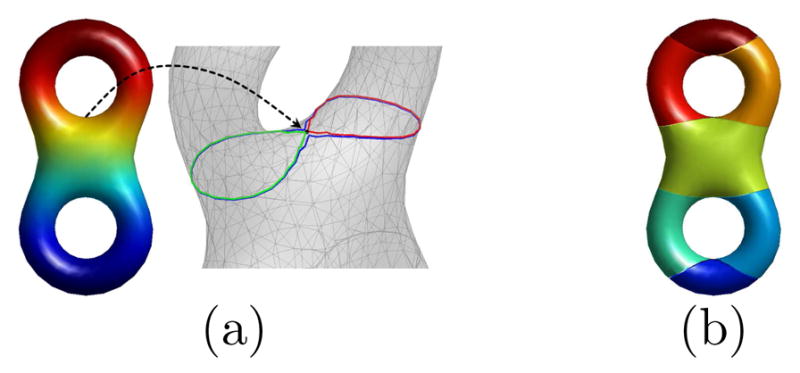
Reeb graph of a LB eigenfunction on a double torus. (a) Level contours in the neighborhood of a saddle point. (b) Edges of the Reeb graph plotted in different colors.

3 Unified Geometry and Topology Correction

For the analysis of a 3D MR image, we denote the lattice of voxels as A = {(i, j, k) ∈ ℤ³|0 ≤ i < I − 1, 0 ≤ j < J − 1, 0 ≤ k < K − 1} and the 3D image as a function A → ℝ. Following the preprocessing steps in [12], we can define an evolution speed F on the lattice A based on tissue classification of MR images, and use the fast evolution algorithm in [10, 13] to find the boundary between two tissue types. Let A_o and A_b denote the object and background region, respectively, and their boundary be represented as a triangular mesh = { , }, where and are the set of vertices and triangles. For each face ∈ , we denote it as the intersection of two boundary voxels: the interior voxel x_o( ) ∈ A_o and the exterior voxel x_b( ) ∈ A_b.

3.1 Paired Boundary Estimate

For topological analysis, we compute a pair of boundary estimates with the evolution speed F. The first boundary satisfies the genus-zero condition and is denoted as = ( , ). The second boundary can have arbitrary topology and is denoted as = ( , ), which is obtained by turning off the topology-preserving condition in the evolution algorithm. Let f be the first non-constant LB eigenfunction on , and R(f) = (C, E) the Reeb graph of f on that we build with the algorithm in section 2. Here C denotes the set of critical points, and E the set of edges. Each edge is represented as $E_i=({SC}_i,{EC}_i,{EV}_i,{LC}_i^s,{LC}_i^e)$, where SC_i, EC_i ∈ C are the start and end node, EV_i ⊂ is the set of vertices belonging to this edge in R(f), ${LC}_i^s$ and ${LC}_i^e$ are the level contours on the boundary of the edge. Using intrinsic Reeb analysis, we can locate outliers and correct them by modifying the evolution speed F to generate an accurate boundary estimation.

3.2 Geometric Outlier Correction

The degree of a node in the Reeb graph is the number of edges that it is either the start or the end node. A node is called a leaf node if its degree is one, and an internal node if its degree is greater than one. The edge connected to a leaf node is called a leaf edge. We detect geometric outliers from the set of leaf edges in the Reeb graph. Let E_i be a leaf edge, ${LC}_i^s$ and ${LC}_i^e$ denote the level contours at the start and end node that are used to generate the edge. Let (EV_i) be the set of triangles connected to the vertices in EV_i, we consider this leaf edge as an outlier if it satisfies two conditions: (1) $\mathit{length}({LC}_i^s)+\mathit{length}({LC}_i^e)<\alpha$; (2) $\mathit{Area}(\mathcal{T}({EV}_i))/(\mathit{length}({LC}_i^s)+\mathit{length}({LC}_i^e))>\beta$, where the parameters α and β are thresholds selected to identify sharp and small outliers. To further localize geometric outliers, we project the mesh onto a subset of four LB eigenfunctions and calculate the area distortion of triangles to measure geometric regularity [10]. For each triangle in , its area distortion ratio is defined as $\mathit{ADF}({\mathcal{T}}_i^F)=\mathit{Area}(T_i^F)/\mathit{Area}({\widehat{T}}_i^F)$, where ${\widehat{T}}_i^F$ is the corresponding triangle of $T_i^F$ on the projected mesh . For an outlier leaf edge, we define the set of outlier triangles as $\mathit{Outlier}({EV}_i)=\{{\mathcal{T}}_i^F\in \mathcal{T}({EV}_i)\mid \mathit{ADF}({\mathcal{T}}_i^F)>\gamma \}$, where γ is a threshold for geometric regularity.

To remove the outlier, we modify the evolution speed F as follows. For each outlier edge E_i, we use the level contour ${LC}_i^s$ and ${LC}_i^e$ to compute:

$$H(E_i)={\int }_{{LC}_i^s}<\mathbf{p}(s)-{\overline{\mathbf{q}}}_i^s,\mathbf{n}(\mathbf{p}(s))>ds+{\int }_{{LC}_i^e}<\mathbf{p}(s)-{\overline{\mathbf{q}}}_i^e,\mathbf{n}(\mathbf{p}(s))>ds$$ (2)

where n is the outward normal on the surface , ${\mathbf{q}}_i^s$ and ${\mathbf{q}}_i^e$ are the mean coordinates of points on ${LC}_i^s$ and ${LC}_i^e$. If H(E_i) > 0, E_i is an outward leaf, we set $F({\mathbf{x}}_o({\mathcal{T}}_i^F))=-1$ for all ${\mathcal{T}}_i^F\in \mathit{Outlier}({EV}_i)$. If H(E_i) < 0, E_i is an inward leaf and we set $F({\mathbf{x}}_b({\mathcal{T}}_i^F))=1$ for all ${\mathcal{T}}_i^F\in \mathit{Outlier}({EV}_i)$.

3.3 Topological Outlier Correction

For topological analysis, we first remove duplicated edges in R(f). For any two edges with the same start and end node, we remove the one with smaller size from R(f) and add it to the set of topological outlier which we denote as TO. After that, we represent the Reeb graph R(f) as a matrix W. For any edge $E_i=(C_{i1},C_{i2},{EV}_i,{LC}_i^s,{LC}_i^e)$, we set W(i1, i2) = #(EV_i), which is the number of vertices on this edge.

For a node C_i in the directed graph W, we use breadth-first-search (BFS) to test if a handle or hole exists. Let j₁, · · ·, j_K denote the set of neighboring nodes of C_i in R(f). For each outgoing edge, we set W(i, j_k) = 0 and perform BFS with C_i as the starting node. This generates a spanning tree PAR_k of nodes reachable from C_i after the removal of the edge from C_i to C_jk. By repeating this process for all outgoing edges at C_i, we generate a set of BFS trees PAR₁, …, PAR_K. The intersection node C_Jmin of these trees is defined as the node with the smallest index j but in all spanning trees. Starting from C_Jmin, we trace backward to the current node C_i on each tree PAR_k and pick the one with the smallest size as a topological outlier and add all edges on this path to TO.

For an edge E_i ∈ TO, we compute the feature H(E_i) using (2). The edge E_i is classified as a handle if H(E_i) > 0 and a hole otherwise. For each handle or hole, we find a cutting path with minimal length. If E_i is a handle, we uniformly sample a set of level contours of the eigenfunction f between the start contour ${LC}_i^s$ and end contour ${LC}_i^e$ of E_i, and pick the one with the least length as the cutting path. For a hole, we combine two geodesic paths to form a cutting path. The first geodesic goes from the start to the end node inside the edge E_i. The second geodesic goes from the start to the end node without passing the edge.

To make cut or fill decisions about topological outliers, we find paired patches on that jointly fill a hole or handle in . For all faces on with their interior voxels in the background region of , we perform a connected component labeling and denote the set of patches as ${CC}^G=\{{CC}_1^G,{CC}_2^G,\cdots \}$. Triangles in different patches are paired if they share a common interior voxel. These triangle pairs are then grouped into paired components ${PC}^G=\{{PC}_1^G,{PC}_2^G,\cdots \}$ according to their paired patch labels in CC^G. For each paired patches, its interior voxels are ${\mathbf{x}}_o({PC}_i^G)$ and they are filled inside to satisfy the genus-zero constraint. A cut decision should be made if either conditions is met:

• Number of voxels $\mathbf{p}\in {\mathbf{x}}_o^T({PC}_i^G)$ classified as CSF is greater than THD_CSF.

• Number of triangles ${\mathcal{T}}_j\in {PC}_i^G$ with ADF( ) > γ is greater than THD_GEO.

The first condition checks if filling a handle/hole needs voxels classified as CSF. The second condition measures the geometric regularity of the filling patches. To cut open a paired component in , we search for a handle or hole with the shortest cutting path that is connected to this paired component. Let CP_i denote the cutting path of this hole or handle and the set of triangles it passes on as (CP_i). To cut open this component, we modify the evolution speed as follows: F(p) = − 1 for p ∈ x_o( (CP_i)).

As an illustration, we plotted the detected outliers on a WM boundary with Reeb analysis in Fig. 2. By iteratively applying the steps in section 3.1, 3.2, 3.3, we can remove both geometric and topological outliers in a unified framework.

Fig. 2.

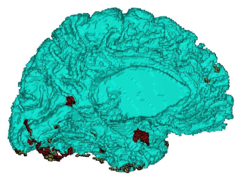
Yellow: geometric outliers; Red: Topological outliers.

3.4 Sub-voxel Accuracy

Let M^G represent the genus-zero, triangular mesh representation of the boundary between high intensity tissue TM_h and low intensity tissue TM_l after the removal of outliers. The pair (TM_h, TM_l) could be (WM, GM) or (GM, CSF). To achieve sub-voxel accuracy, we estimate locally the isosurface location between the two tissue types at each vertex of . Let denote the shift of all vertices to their locally estimated iso-surface location, we compute the final vertex coordinates by minimizing the energy

$$E={\left|\right|\mathbf{x}+S_{\mathcal{V}}-\widehat{\mathbf{x}}\left|\right|}^2+\eta {\left|\right|\mathrm{\Delta }\widehat{\mathbf{x}}\left|\right|}^2$$ (3)

where x is the vector of coordinates of all vertices, Δ is the discrete Laplacian matrix of the mesh, and η is a regularization parameter. The solution of this quadratic problem gives the coordinates of vertices on the final cortical surface:

$$\widehat{\mathbf{x}}={(I+\eta {\mathrm{\Delta }}^{\prime }\mathrm{\Delta })}^{-1}(\mathbf{x}+S_{\mathcal{V}}).$$ (4)

4 Experimental Results

In this section, we demonstrate our method and compare with FreeSurfer [2], which is widely used in brain imaging research, on two large datasets. The first dataset includes skull-stripped MR images of 50 normal controls(NC) and 50 Alzheimer’s disease (AD) patients from ADNI [6]. The second dataset includes 100 skull-stripped MR images from ICBM [7] and it has a wide age range from 19 to 80. For all images, the same set of parameters are used in our method: α = 100mm, β = 5, γ = 100, THD_CSF = 5, THD_GEO = 5, η = 10.

In the first experiment, we present detailed comparisons using one MR scan of an AD patient in ADNI. We applied our method and FreeSurfer to reconstruct the WM and GM surfaces on both hemispheres. Computationally our method took around 3 hours and is much more efficient than FreeSurfer, which took more than 10 hours. In Fig. 3, the left hemispherical WM surfaces reconstructed by both methods are plotted. In regions highlighted by the dashed curves, we can see that our method produces more complete reconstruction of the boundary, which is better illustrated with the intersections of surfaces and two axial slices shown in Fig. 3(c). The left hemispherical GM surfaces reconstructed with our method and FreeSurfer are plotted in Fig. 4(a). The intersections of the surfaces with two sagittal slices shown in Fig. 4(b) illustrate that our surface can better capture deep sulcal regions.

Fig. 3.

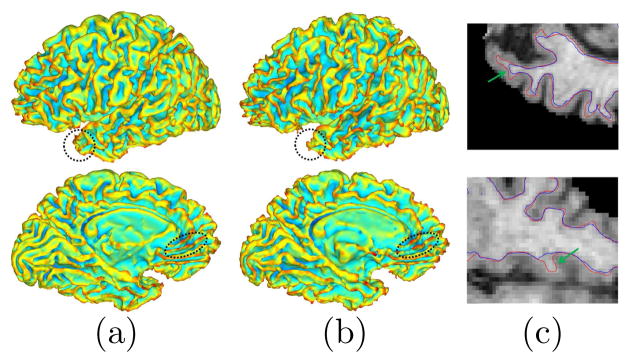
A comparison of WM surfaces. (a) Our result. (b) FreeSurfer result. (c) Intersection of image slices with highlighted regions on surfaces. Red: our method. Blue: FreeSurer.

Fig. 4.

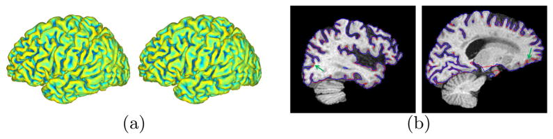
A comparison of GM surfaces. (a) Left: Our result. Right: FreeSurfer result. (b) Intersection of sagittal slices with surfaces. Red: our method. Blue: FreeSurfer.

In the second experiment, we applied both our method and FreeSurfer to the MR images of 50 NC and 50 AD from ADNI. Using a general surface mapping algorithm [14], we projected the gyral labels of the LPBA40 atlas [15] to all left hemispherical surfaces. For each gyrus, we computed the average gray matter thickness and tested group differences between NC and AD using two tailed t-tests. The p-values from our method and FreeSurfer are plotted in Fig. 5. Our method can achieve more significant p-values on 18 of the 24 gyral regions.

Fig. 5.

P-value maps of gyrus-based thickness differences between NC and AD. (a) Our results. (b) FreeSurfer results.

In the third experiment, we applied our method and FreeSurfer to the 100 MR images from the ICBM database and used the results to model the decrease of gray matter thickness in normal aging. The reconstructed surfaces were first automatically labeled into gyral regions with the same approach in the second experiment. Regression analysis was then applied to the mean thickness of each gyrus against subject age. The results are shown in Fig. 6, where the rates of decrease are plotted in Fig. 6(a) and (b), and the p-values of the regression analysis are plotted in Fig. 6(c) and (d). We can see that our method can achieve statistically much more significant results on all gyral regions.

Fig. 6.

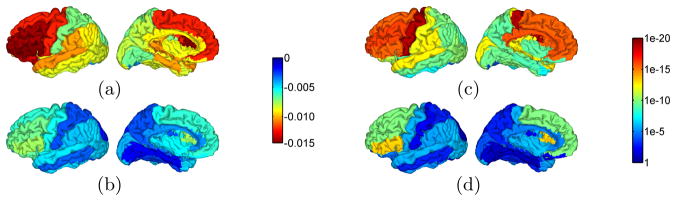
Regression analysis of gray matter thickness and normal aging. (a) Rate of decrease from our results. (b) Rate of decrease from FreeSurfer results. (c) P-value maps of our results. (d) P-value maps of FreeSurfer results.

5 Conclusions

In this paper we developed a novel approach for the unified correction of geometric and topological outliers in cortical surface reconstruction. Comparisons with a state-of-the-art tool showed that our method is computationally more efficient and can achieve better performance in population studies. The Reeb analysis framework developed here is general and can be valuable for general surface reconstruction and analysis problems.

References

- 1.Mangin JF, Frouin V, Bloch I, Regis J, Lopez-Krahe J. From 3D magnetic resonance images to structural representations of the cortex topography using topology preserving deformations. J MATH IMAGING VIS. 1995;5(4):297–318. [Google Scholar]
- 2.Dale AM, Fischl B, Sereno MI. Cortical surface-based analysis i: segmentation and surface reconstruction. NeuroImage. 1999;9:179–194. doi: 10.1006/nimg.1998.0395. [DOI] [PubMed] [Google Scholar]
- 3.Shattuck D, Leahy R. BrainSuite: An automated cortical surface identification tool. Med Image Anal. 2002;8(2):129–142. doi: 10.1016/s1361-8415(02)00054-3. [DOI] [PubMed] [Google Scholar]
- 4.Han X, Pham DL, Tosun D, Rettmann ME, Xu C, Prince JL. CRUISE: Cortical reconstruction using implicit surface evolution. NeuroImage. 2004;23:997–1012. doi: 10.1016/j.neuroimage.2004.06.043. [DOI] [PubMed] [Google Scholar]
- 5.Li G, Nie J, Wu G, Wang Y, Shen D. Consistent reconstruction of cortical surfaces from longitudinal brain mr images. NeuroImage. 2012;59(4):3805–3820. doi: 10.1016/j.neuroimage.2011.11.012. [DOI] [PMC free article] [PubMed] [Google Scholar]
- 6.Mueller S, Weiner M, Thal L, Petersen RC, Jack C, Jagust W, Trojanowski J, Toga A, Beckett L. The Alzheimer’s disease neuroimaging initiative. Clin North Am. 2005;15:869–877. xi–xii. doi: 10.1016/j.nic.2005.09.008. [DOI] [PMC free article] [PubMed] [Google Scholar]
- 7.Mazziotta JC, Toga AW, Evans AC, et al. A probabilistic atlas and reference system for the human brain: international consortium for brain mapping. Philos Trans R Soc Lond B Biol Sci. 2001;356:1293–1322. doi: 10.1098/rstb.2001.0915. [DOI] [PMC free article] [PubMed] [Google Scholar]
- 8.Reuter M, Wolter FE, Shenton M, Niethammer M. Laplace-beltrami eigenvalues and topological features of eigenfunctions for statistical shape analysis. Computer-Aided Design. 2009;41(10):739–55. doi: 10.1016/j.cad.2009.02.007. [DOI] [PMC free article] [PubMed] [Google Scholar]
- 9.Qiu A, Bitouk D, Miller MI. Smooth functional and structural maps on the neocortex via orthonormal bases of the Laplace-Beltrami operator. IEEE Trans Med Imag. 2006;25(10):1296–1306. doi: 10.1109/tmi.2006.882143. [DOI] [PubMed] [Google Scholar]
- 10.Shi Y, Lai R, Morra J, Dinov I, Thompson P, Toga A. Robust surface reconstruction via Laplace-Beltrami eigen-projection and boundary deformation. IEEE Trans Med Imag. 2010;29(12):2009–22. doi: 10.1109/TMI.2010.2057441. [DOI] [PMC free article] [PubMed] [Google Scholar]
- 11.Cole-McLaughlin K, Edelsbrunner H, Harer J, Natarajan V, Pascucci V. Loops in Reeb graphs of 2-manifolds. Discrete Comput Geom. 2004;32(2):231–44. [Google Scholar]
- 12.Shi Y, Lai R, Toga A. CORPORATE: Cortical reconstruction by pruning outliers with Reeb analysis and topology-preserving evolution. Proc IPMI. 2011:233–44. doi: 10.1007/978-3-642-22092-0_20. [DOI] [PubMed] [Google Scholar]
- 13.Shi Y, Karl WC. A real-time algorithm for the approximation of level-set-based curve evolution. IEEE Trans Image Processing. 2008;17(5):645–657. doi: 10.1109/TIP.2008.920737. [DOI] [PMC free article] [PubMed] [Google Scholar]
- 14.Shi Y, Lai R, Gill R, Pelletier D, Mohr D, Sicotte N, Toga A. Conformal metric optimization on surface (CMOS) for deformation and mapping in Laplace-Beltrami embedding space. Proc MICCAI. 2011;2:327–34. doi: 10.1007/978-3-642-23629-7_40. [DOI] [PubMed] [Google Scholar]
- 15.Shattuck D, Mirza M, Adisetiyo V, Hojatkashani C, Salamon G, Narr K, Poldrack R, Bilder R, Toga A. Construction of a 3D probabilistic atlas of human brain structures. NeuroImage. 2008;39(3):1064–1080. doi: 10.1016/j.neuroimage.2007.09.031. [DOI] [PMC free article] [PubMed] [Google Scholar]