The application of information theory to biochemical signaling systems

Abstract

Cell signaling can be thought of fundamentally as an information transmission problem in which chemical messengers relay information about the external environment to the decision centers within a cell. Due to the biochemical nature of cellular signal transduction networks, molecular noise will inevitably limit the fidelity of any messages received and processed by a cell’s signal transduction networks, leaving it with an imperfect impression of its environment. Fortunately, Shannon’s information theory provides a mathematical framework independent of network complexity that can quantify the amount of information that can be transmitted despite biochemical noise. In particular, the channel capacity can be used to measure the maximum number of stimuli a cell can distinguish based upon the noisy responses of its signaling systems. Here, we provide a primer for quantitative biologists that covers fundamental concepts of information theory, highlights several key considerations when experimentally measuring channel capacity, and describes successful examples of the application of information theoretic analysis to biological signaling.

Introduction

In their in vivo environment, cells are constantly awash in a sea of hormones, cytokines, morphogens, and other receptor ligands released by other cells. Each of these molecular signals can be thought of as being sent with the intent of communicating a specific message or action for the receiving cell to perform. Within the recipient cell, the information contained within the chemical messages must be captured and processed by the cell’s biochemical circuitry, which typically involves feedback loops, crosstalk, and delays. These control functions are commonly executed by dedicated sets of kinases and transcription factors to ensure that the appropriate cellular response is activated. Since the mechanisms behind this complex function are biochemical in nature, molecular noise can greatly hamper the propagation of signals [1–3]. As a result, the message can get distorted and cells may not be able to acquire a precise perception of their surroundings.

Biological noise can perhaps more adequately described as stochastic cell-cell variability and can be experimentally observed by sampling the distribution of responses by a group of genetically identical cells exposed to the same stimulus. If, for example, the distribution of responses elicited by a weak stimulus overlaps with the distribution elicited by a strong stimulus, a cell whose response value falls within the overlap will not be able to discern with absolute certainty which stimulus was present (figure 1A). This inability to resolve distinct stimuli represents a loss of information about the input. Traditional metrics for noise related to the standard deviation or variance primarily quantify the magnitude of noise and do not directly indicate the degree to which noise hampers the discrimination of different inputs. Likewise, both deterministic and stochastic mathematical models, although able to capture dynamic trends, require a priori knowledge or assumptions of the underlying molecular mechanisms and ultimately fail to describe how signaling fidelity is affected by variability. In order to quantify the degree to which noise affects the fidelity of the message, or specifically to determine what a biological signaling system can or cannot communicate accurately, it is useful to turn to information theory.

Figure 1. (A) Noise can limit the amount of information a cell can obtain about a stimulus.

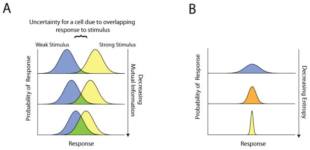
The magnitude of noise is evidenced in the breadth of the probability distribution of the response to a given stimulus. For sufficiently large noise, a cell which can encounter strong or weak stimuli cannot use its response to discern which stimulus was encountered with absolute precision. Consequently, from the cell’s perspective, noise leads to a loss of information about the input. The amount of mutual information between the stimulus and cellular response also suffers such that the greater the overlap between distributions, the less mutual information is communicated. (B) Entropy can be understood as a measure of dispersion. A wider probability distribution corresponds to an increase in the uncertainty of the cellular response and consequently, entropy.

Originally developed by Claude Shannon for the purpose of data compression and the analysis of man-made communication systems, information theory provides a mathematical framework to quantify the amount of information that can be transmitted through a noisy communication channel. A differentiating strength of this type of analysis, especially pertinent in cell signaling, is that only input and output measurements are required, thereby obviating the need for a detailed understanding of the signaling system. With information theory, any complex system can be reduced to a black box communications channel and analyzed. When details of the underlying system are available, they can be included as part of the analysis, leading to an even deeper understanding. Some examples of biological systems that have benefitted from such an analysis include neural networks [4] and, more recently, gene regulation networks [5, 6], particularly in developmental biology [7], and signal transduction networks [8].

In this review, we aim to provide a basic background and guide for quantitative biologists interested in using information theory in the analysis of signal and information transduction in noisy biochemical networks. Specifically, we endeavor to provide readers having an undergraduate-level understanding of probability with a basic understanding of entropy and mutual information, as needed to appreciate applications of information theory to biology. We refer the reader to excellent texts [9, 10] for more in-depth discussions of these core concepts, which due to space constraints, could not be included here. Additionally, for summaries of the application of information theory in biology we recommend the following recent reviews [11, 12].

Key concepts from information theory

In order to quantify how much information can be transmitted, we must first define it. In Shannon’s theory, information is conceptually considered to be knowledge that enables the state of a system (or signal or input) to be distinguished from among many available potential states. Examples include whether a coin flip turns up heads or tails, or whether a roll of a die is 1, 2, 3, 4, 5, or 6, or (as Paul Revere famously employed) whether one light is lit to signal a land invasion versus two lights to signal invasion by sea. The more states that are available for selection, the more information can be obtained when the selection is made. Importantly, in this model of information, the meaning or identity of a state is irrelevant. It only matters that each state can be encoded as a unique symbol, such as heads/tails, the numbers 1 through 6, or one or two lights.

As a consequence of the above definition, any system capable of taking on multiple states can be a source of information, and that state can be mathematically represented as a random variable that can take on multiple values. If we are initially uncertain about the value of this random variable, but then later ascertain its value, we will have resolved the system’s state and thus gained information. The amount of information that can be gained, or equivalently the amount of uncertainty associated with the random variable that can be reduced, can be quantified by the Shannon entropy which is described further below.

The analysis of how well information can be transmitted relies on the concept of a communication channel, which is a system that links an input source of information to some output (figure 2A). Any channel can be mathematically represented by a random variable for the input and another random variable for the output, where the values of the two variables depend on each other. Consequently, measuring the output value can help resolve the input value, and the amount of information thus gained can be quantified using the mutual information, described below.

Figure 2. (A) Schematic of a communication channel.

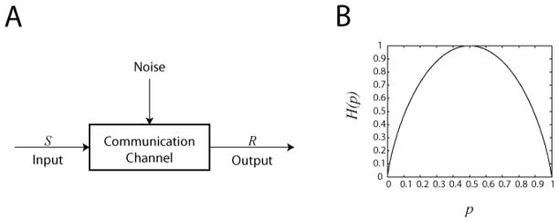
A basic communication channel can be described by an input random variable S connected by a channel to a random variable output R such that the outcome of R is dependent on S subject to the distorting influence of noise. In information theory the complexity of the channel can be represented as a “black box”, since the internal details are fully captured by the joint distribution between R and S. (B) Entropy as a function of a Bernoulli random variable with probability p. This concave down graph illustrates that entropy is at its maximum when all outcomes are equally probable (p = 0.5) and at a minimum when the outcome is predetermined (p = 0 or 1).

Entropy

A central concept to information theory is the Shannon entropy, a separate concept from the thermodynamic entropy. The Shannon entropy (hereafter referred to simply as entropy) quantifies how unpredictable the value of a random variable is, and hence can be thought of as a measure of uncertainty. For a discrete random variable X which can take on the values x₁, x₂, .., x_n, with the respective probabilities p(x₁), p(x₂), …, p(x_n), the entropy is defined as [9]

$$H(X)=-\sum _{i=1}^{n}p(x_i){log}_{2}p(x_i)$$ [1]

We have chosen, by the usual convention, to define entropy using a base 2 logarithm so that the entropy is measured in bits. Note also that since each of the p(x_i) is between zero and one inclusive, each term in the sum is non-positive (taking, by convention, the value of 0 log 0 to be identically zero), and thus entropy is necessarily non-negative.

A few case examples can help to demonstrate that this formula indeed provides an intuitive measure of uncertainty. In the first example, let X be the outcome of a flip of an evenly weighted coin. This random variable has two outcomes each with probability of ½, i.e. p(x₁) = p(x₂) = ½. Thus, the entropy of X is

$$H\left(X_{\mathit{fair}\mathit{coin}}\right)=-{log}_2\frac{1}{2}=1\text{bit}$$

The 1 bit entropy is consistent with the uncertainty associated with the two equally probable outcomes for the flip of a fair coin.

Now, in the second example, consider instead the example of rolling a fair 6-sided die. In comparison to the fair coin, there are more outcomes (also equally probable), hence we would expect the entropy to be greater. Indeed, for this example, p(x₁) = p(x₂) = … = p(x₆) = 1/6, so that

$$H\left(X_{\mathit{fair}\mathit{die}}\right)=-{log}_2\frac{1}{6}=2.59\text{bits}.$$

As anticipated, the value of 2.59 bits confirms our expectation that the greater number of possible outcomes confers higher entropy to rolling of a fair die than to flipping of a fair coin.

In our third example, consider the flip of an unfair coin. If the coin is now weighted so that it is three times as likely landing heads instead of tails, the entropy of a single coin flip decreases from 1 bit to 0.81 bits.

$$H\left(X_{\mathit{unfair}\mathit{coin}}\right)=-\frac{1}{4}{log}_2\frac{1}{4}-\frac{3}{4}{log}_2\frac{3}{4}=0.81\text{bits}$$

The reduction in entropy reflects a greater degree of certainty as to the outcome of the flip of the unfair coin compared to a fair coin. More generally, we can compute entropy as a function of the probability of landing heads, which yields a concave down graph (figure 2B). The plot shows that the entropy is maximized when the probability is exactly 50%, and provides a clear example of a more general property of entropy: it is maximized when all outcomes are equally probable. Stated differently, when all outcomes are equally likely, then uncertainty is at its greatest.

Frequently, new users of information theory are confused as to the interpretation of partial bits. In computers, information storage is measured in a whole number of bits, but in information theory entropy (and related quantities) can take on non-integer values. Thus, 0.81 bits of entropy can be interpreted as being equivalent to a system that can take on between 1 and 2 states.

Continuing the example of an unfair coin, in the extreme, if the coin can only land on heads then the entropy is −1log₂ 1 − 0log₂ 0 = 0. The zero entropy reflects the fact that in this fourth example, the random variable can only take on one predetermined value and thus there is no uncertainty in its value. This is an example of entropy taking on its lowest possible value (recall from above that the entropy is non-negative).

Extending the concept of Shannon entropy towards biology, we again imagine an experiment in which a population of cells is exposed to various stimuli and the resulting individual cell responses are recorded. We may observe that, depending on the stimulus, the population of cells may exhibit relatively wide or narrow response distributions (figure 1B). The response entropy can then be used as a metric of dispersion, because, as the variance of the response of a population of cells increases, there is higher uncertainty as to what response value an individual cell will take on and hence, greater associated entropy.

Together, these examples demonstrate that the entropy is an intuitive measure of the uncertainty associated with a random variable, and is a simple function of the number of possible states and the probabilities associated with those states. The specific form given in Eq. 1 can be shown to be required for any measure of uncertainty which satisfies certain sensible axioms, particularly continuity, symmetry (the entropy does not depend on the assignment of the x_i’s), maximality (entropy is maximized for a uniform distribution), and additivity (if the possible outcomes are partitioned into subsets, the overall entropy is the probability-weighted sum of the entropy of subsets) [9]. Armed with this understanding of entropy, we now turn to a special use of the entropy: mutual information.

Mutual Information

A communication channel, such as a phone cable, fiber-optic line, or biochemical pathway, allows information to be transmitted from one place to another. Regardless of its underlying physical basis or complexity, any channel can be reduced to a “black box” that maps an input to an output. Because the input is not known a priori it can be considered to be a random variable, thus the output whose value depends on the input is also a random variable. Useful communication occurs if knowing the output value allows the input value sent through the channel to be fully or partially determined.

Mutual information quantifies this concept in terms of the amount of information that the value of one random variable contains about the value of another random variable. Using S to represent the input (signal or sender, depending on context) and R to represent the output (response or receiver), we can define their mutual information I(R;S) as:

$$I(R;S)=H(S)-H(S\mid R)$$ [2]

where H designates entropy. As discussed above, entropy is a measure of uncertainty, thus H(S) can be interpreted to be the overall uncertainty one has about the input S, and H(S|R) is the residual uncertainty about S after the value of the response R is known. Hence, the above definition can be interpreted to mean that mutual information is the reduction in the uncertainty about S given the value of R. Equivalently, the mutual information measures how accurately the input value can be determined based upon the output value.

To illustrate how mutual information measures communication accuracy, consider the simple example in which Samantha relays the result of a fair coin flip (S) over her phone to Roy who then records the result (R). For a fair coin flip, H(S) = 1 bit since both sides are equally probable as discussed above. In the first scenario, assume that the phone has no static and there is never any miscommunication between Samantha and Roy. In this case, R tells us exactly the value of S. When R is heads, S is always heads; and when R is tails, S is always tails. Hence in this example there is no residual uncertainty about S once R is known and H(S|R) = 0 bits. Together, the information that R provides about S is I(R;S) = 1 − 0 = 1 bit, as one would expect.

In the second scenario, imagine that the phone has static and there is sometimes miscommunication, e.g. suppose that 25% of the time Roy records the incorrect result. Then, knowing the value of R still leaves some uncertainty as to the value of S. Specifically, the conditional entropy is

$$\begin{array}{l}H(S\mid R)=P(R=\text{heads})H(S\mid R=\text{heads})+P(R=\text{tails})H(S\mid R=\text{tails})\\ =\frac{1}{2}(0.81)+\frac{1}{2}(0.81)\\ =0.81\end{array}$$

where both H(S|R=heads) and H(S|R=tails) correspond to the unfair coin example whose entropy was computed to be 0.81 bits in the previous section. Together, this means that R provides only I(R;S) = 1 − 0.81 = 0.19 bits of information about S. As expected, the mutual information is lower compared to the case of perfect communication.

In the third scenario, consider the extreme case in which Roy cannot at all tell what Samantha says on the phone and must guess randomly as to the result of the coin flip. It is easy to determine that the residual uncertainty about S is quite high:

$$\begin{array}{l}H(S\mid R)=P(R=\text{heads})H(S\mid R=\text{heads})+P(R=\text{tails})H(S\mid R=\text{tails})\\ =\frac{1}{2}(1)+\frac{1}{2}(1)\\ =1\end{array}$$

and hence I(R;S) = 1 − 1 = 0 bits. The mutual information in this case implies zero transmission of information, matching with the expected result for this example. Together, these three examples help illustrate the concept that mutual information measures communication accuracy in terms of a reduction in uncertainty.

We can extend the idea of mutual information to biochemical signaling processes, by continuing with our previous example of entropy in cellular response distributions. The population of cells mentioned earlier is now subject to different stimuli and seeking to identify them. In particular, consider one strong and one weak stimuli generating corresponding response distributions (figure 1A). If we were to randomly select a cellular response from either distribution and then attempt to resolve which stimulus was used, it is evident that the more the response distributions are separated the greater the accuracy in predicting the original stimulus. Conceptually, mutual information measures this accuracy. Thus, a large overlap between the weak and strong stimulus response distributions confounds our ability to discern the original stimulus leading to a corresponding drop in the mutual information between the stimulus and cellular response.

Mutual information has additional mathematical properties which are relevant to understanding its application to biological systems. First, by substituting in the definition of entropy, and expanding and rearranging the probabilities, we can arrive at an alternative definition of mutual information:

$$\begin{array}{l}I(R;S)=H(S)-H(S\mid R)\\ =-\sum _{S}p(s){log}_{2}p(s)+\sum _{R}p(r)\sum _{S}p(s\mid r){log}_{2}p(s\mid r)\\ =-\sum _S\sum _{R}p(s,r){log}_{2}p(s)+\sum _S\sum _{R}p(s,r){log}_{2}p(s\mid r)\\ =\sum _S\sum _{R}p(s,r){log}_2\frac{p(s\mid r)}{p(s)}\\ =\sum _S\sum _{R}p(s,r){log}_2\frac{p(s,r)}{p(s)p(r)}\end{array}$$ [3]

The alternative definition, given by the last equation above, is symmetric with respect to R and S. This symmetry implies that R gives as much information about S as S gives about R. Since this implies that I(R;S) and I(S;R) are identical, we have used the conventional semicolon notation to indicate that the order of the arguments within the parentheses is irrelevant. Mathematically, another important consequence of the symmetry is that

$$I(R;S)=H(R)-H(R\mid S)$$ [4]

This relation is critical since we usually wish to quantify the reduction in uncertainty about the signal provided by the response (represented the former equality), but it is usually far easier to experimentally measure the distribution of responses (represented by the latter equality).

Next, we note that the lower bound of mutual information is zero. This lower bound is achieved if the quantities S and R are statistically independent of each other, for then p(s, r) = p(s)p(r) and the logarithm in Eq. 3 is always zero. Such independence might be achieved in the case of a communication channel affected by large amount of noise (see the third example above), and for such channels it is sensible that if there is no statistical dependence between the input and output, the value of one cannot provide any information (reduction in uncertainty) about the other. The converse is also true, that if their mutual information is zero then S and R are statistically independent. A practical implication of this property is that, outside its use in quantifying information transmission fidelity, mutual information can be used as a general tool for detecting whether there is any statistical dependency between two variables of interest.

At the other extreme, the upper bound of mutual information is the smaller of H(S) and H(R). The proof stems from the fact that entropy cannot be negative, so H(S|R) ≥ 0 thereby implying that I(R;S) ≤ H(S), and symmetrically, I(R;S) ≤ H(R). This upper bound can be reached, for instance, if S|R can only take on a single outcome, implying unambiguous identification of the signal that generated the specific response. In such a case H(R|S) will equal zero and I(R;S) will equal H(S) (see the first example provided above). Conceptually, the upper bound is only reached when there is no “noise” in the communication channel between S and R, such that the response leaves no residual uncertainty about the signal. More importantly, the upper bound also implies that the range of values that the input and output can take can limit the effectiveness of the communication channel. For instance, if we have a signal S that can take on 1,000,000 values (an entropy as high as log₂ 1,000,000 ≈ 20 bits) but the output R that can only take on one of two values (entropy at most 1 bit) then the mutual information between S and R is necessarily 1 bit or less. As a result, a communication channel relying on a rich signal but poor output, or vice versa, can be limited in its ability to transmit information.

Notably, in most real world examples, there is a statistical dependence between S and R but the relationship is not “noiseless”. In such cases, the mutual information is positive but not as large as either the entropy of S (or R). The exact amount of mutual information will depend on the structure of the noise, that is, the particular way in which R is a noisy representation of S. In the biological context, the noise may include both intrinsic and extrinsic noise as all sources of noise can potentially confound accurate signaling. The effect of noise is fully encapsulated in the joint probability distribution between S and R, which as shown in Eq. 3, also fully determines the mutual information. Thus, to compute the mutual information for a real world communication channel we must be able to measure the complete joint distribution between its input and output. Indeed, we note that one of the fundamental abstractions in information theory is that any channel can be represented by such a joint distribution, thus enabling an information theoretic analysis to be performed when the input-output properties of the channel are known but the underlying mechanisms generating those properties are unknown. Thus, by carefully choosing the input and output of interest, one can apply information theory to a broad variety of cell signaling systems, although one must be mindful of whether the properties of the channel would change depending on the context (e.g., whether the channel properties might be different in different cell types, or whether it might be retroactively affected by the presence of downstream processes, etc.).

Channel Capacity

The mutual information is the amount of information transmitted through a channel for a particular input probability distribution, and is not purely an intrinsic property of the channel. To see why, note that the mutual information I(R;S) is fully specified by the joint distribution p(r, s), which can be decomposed as the product of two probabilities: p(r, s) = p(r|s)p(s). The conditional distribution p(r|s) reflects uncertainty resulting from noise in the communication channel and is a property of the channel itself. In comparison, the marginal distribution p(s) reflects the range of the signals imposed on the channel which might be different for different uses of the channel. In other words, p(s) is a property of the source of the signal rather than a property of the channel itself.

For many real-world communication channels, it can be of interest to know the maximum amount of information that can possibly be transmitted through the channel. For a given channel (i.e. for a fixed p(r|s)), this quantity is known as the channel capacity C(R;S) and is mathematically defined as

$$C(R;S)={sup}_{p(s)}I(R;S)$$ [4]

In other words, the channel capacity is the mutual information maximized over all possible distributions of the signal (i.e., all possible signal sources or uses). Thus, capacity is effectively the data bandwidth and is an intrinsic property of the channel itself. The relevance of the capacity is further bolstered by the Noisy Channel Coding Theorem, a fundamental result in information theory. This theorem states that despite some degree of noise in the system a message can be sent across the channel and properly discriminated from other potential messages with an arbitrarily small amount of error, given that the entropy of the potential messages (i.e., the information source) is below the channel capacity. For an information source with an entropy greater than the capacity, there exists no way to transmit it so that messages can be discriminated from each other in an errorless manner. Thereby, the theorem ensures that capacity places a hard upper bound to how accurately data can be transmitted through a channel. Turning back to our original example, if Samantha would like to communicate to Roy the result of a die roll using a channel with a binary output, the Noisy Channel Coding Theorem would confirm our beliefs that there exists no way to do so in an errorless manner as the entropy of the die is ~2.59 bits which is greater than the 1 bit capacity of the binary channel.

We note that for many biological signaling channels, p(r|s) can be readily experimentally measured, whereas p(s) cannot be easily estimated, particularly if S corresponds to commonly very low ligand concentrations and infrequent signaling events. Hence, the amount of information corresponding to a particular signal source can be difficult to evaluate. However, channel capacity can be easily inferred by determining which p(s) yields the maximum amount of information. Typically, p(r|s) can be sampled by providing a controlled input stimulus to the system and measuring the distribution of responses, which can then be repeated for many different stimulus values. Such an experiment implicitly requires imposing an artificial set of stimuli on the biological system of interest. On the other hand, the relevant p(s) is the natural frequency at which each stimulus value would be encountered by the system. The frequencies may be unknown or, at present, not easily experimentally determined. Nonetheless, for biological channels the capacity may yield insights as to the magnitude of the actual amount of information transmitted, because under the efficient coding hypothesis, biological systems whose primary function is communication can be expected to have evolved to be optimally matched to the information sources that feed them [13]. For instance, in the anterior-posterior patterning system of the embryos of the Drosophila melanogaster fruit fly, the measured mutual information between an input morphogen signal and an output transcription factor was ~90% of the capacity of the system [7] (see below for further discussion). Thus, examination of the maximum capability of a biological system may shed light on its actual data throughput.

Rate Distortion Theory

Often any improvement in the capacity or quality of a communication channel comes at an associated cost (e.g., increased energy required), or alternatively it may be that an errorless communication channel would be impractical or unfeasible to construct. In such scenarios, cognizance of the relationship between the increase in the amount of tolerable channel distortion and the corresponding decrease in required channel capacity would aid in the understanding of biological communication channels. Fortunately, Rate Distortion Theory, a branch of information theory, provides a mathematical framework to examine the trade-off between capacity and the acceptable error (i.e., distortion) limit D.

Rate distortion analysis is performed in the context of a specific distortion function, which measures the error between the sent and received message. For instance, if the sent message is a scalar s and the received message is a scalar r, then a commonly used distortion function d(s,r) is the square of the difference of the sent and received message, d(s, r) = (s − r)².

The rate distortion function R(D) is then defined as the minimum amount of mutual information required to ensure that the average level of distortion is less than or equal to D. Mathematically, this is represented as:

$$R(D)={\mathit{min}}_{p(r\mid s):{\sum }_{(r,s)}p(s)p(r\mid s)d(s,r)\le D}I(S;R)$$

We note that the choice of the distortion function is important as differing measures of distortion will cause the minimization to often arrive at non-identical results. A major result of rate distortion theory is that the capacity of a communication channel must be at least R(D) in order to ensure that the average distortion is less than or equal to D. Furthermore, R(D) is a continuous non-increasing function, thus if the acceptable level of error is increased then the required capacity stays the same or decreases.

In a typical application of rate distortion theory, Roy and Samantha are once again are attempting to relay the results of a coin flip over a telephone line having some degree of static. In this scenario, they have an option of incrementally improving the communications channel at an associated economic cost to reduce the chance of miscommunication. Rate distortion theory helps solve the problem of determining the minimal channel quality such that the communication error does not exceed an amount that is acceptable to both parties.

Data Processing Inequality

Finally, we discuss the data processing inequality, which essentially states that at every step of information processing, information cannot be gained, only lost. More precisely, for a Markov chain X → Y → Z, the data processing inequality states that I(X;Z) ≤ I(X;Y). That is, Z contains no more information about X as Y does. Colloquially, the data processing inequality is analogous to the children’s game of “broken telephone”. As individuals are lined up and told to pass a message by whispering it to the next person in line, the addition of any extra people can only serve to distort the original message but not improve upon it hence the “broken telephone”.

The relevance of the data processing inequality is twofold. First, it places bounds on the performance of a biological system that contains multiple communication channels in series. For instance, consider X → Y to represent cytokine signaling to a transcription factor and Y→ Z to represent transcription factor signaling to the concentration of an expressed protein. Assuming no other sources of information, then the amount of information that the expressed protein (Z) provides about the cytokine signal (X) cannot be more than the information that the transcription factor (Y) provides about the cytokine (X). If the information between X and Y is particularly limiting, this can place strict bounds on the fidelity of the response Z.

Second, the data processing inequality has implications for experimental measurements. For instance, consider the chain S (signal) → R (actual response) → R′ (measured response). Although an experimentalist might wish to quantify the mutual information between the signal and actual response, I(S;R), she is confined to measuring I(S;R′). For I(S;R′) to be close in value to I(S;R) the noise between R and R′ resulting from experimental error must be minimal. Thus, it is critical to pay close attention to the degree of experimental noise when attempting to measure mutual information.

Considerations when experimentally measuring channel capacity

Experimental noise

As noted in the section on the data processing inequality above, experimental measurements are imperfect assessments of biological realities. Mutual information is a quantity that depends on the variability of responses, but this variability may be artifactually augmented by experimental noise. Thus, the capacity of a system can be severely underestimated if steps are not taken to minimize experimental contributions to the observed variability.

Every experimental technique and experimental apparatus can in principle add noise to the measurements. For instance, for microscopy-based measurements, some considerations include uniformity in sample preparation, the choice of focal plane, fluctuations in light source intensity, image processing, etc [14]. When possible, experiments should be devised to measure the effect of each potential source of variability on the measured response. An example of such an experiment would be to systematically vary the focal plane and determine quantify its effect on the image of interest.

Alternatively, one can attempt to devise an assay which measures the total experimental contribution to variability. Such an assay would typically require simultaneous measurement of the response of interest using two largely independent methods. In our studies of tumor necrosis factor (TNF) signaling using immunofluorescence readouts, we employed two methods [8]. One method was to image expressed green fluorescent protein (GFP) molecules that are immunostained using anti-GFP antibodies. The direct fluorescence and immunofluorescence both provide quantitative measures of GFP concentration, and absent any experimental noise, when plotted against each other, the data will lie on a straight line. In our system, we found that the two measurements were strongly correlated with each other (ρ~ 0.95), indicating that just ~5% of the variability (standard deviation) of the immunofluorescence readout could be ascribed to experimental causes. In a second assay, we simultaneously stained for the response protein (NF-κB) using two antibodies. These antibodies were chosen to be specific to different epitopes to prevent cross-interference. Analysis of the correlation between the two antibody measurements confirmed that ~5% of the observed variability was experimental in nature and the rest was likely to be true biological variability.

Bias

After the experimental noise has been sufficiently minimized, one can proceed to measurements of entropy and mutual information on experimental data. First, we note that most experimental data lies on a continuous spectrum whereas the formulas outlined above apply only for discrete data, hence the data must be binned. (There are analogous definitions for the entropy and mutual information of continuous-valued variables, however, well-established numerical methods based on the continuous formulae are not currently available.) The choice of the number of bins and location of bin boundaries can be an important consideration, but here we set this issue aside in favor of discussing a more critical issue, that of numerical bias. We refer the reader to other sources [8, 15, 16] for details regarding binning.

To understand the origin of the bias, recall that entropy depends on the range of values that a random variable can realize. A finite data sample, by its nature, will not reflect the full range of the underlying distribution and will give the perception that the distribution is thinner than it really is. Consequently, the entropy computed on a finite data sample will be smaller than the true entropy, although this negative bias will diminish as the sample size increases. Similarly, the conditional entropy H(R|S) is also negatively biased but more strongly than H(R) since by definition the sample used to estimate H(R) is larger than the sample used to estimate H(R|S) (the sample for R is the aggregate of all R|S samples). Thus, from the equation I(R;S) = H(R) − H(R|S) it is evident that estimated mutual information will be positively biased, although again this bias will diminish as the sample size increases.

Depending on the system, the bias confounding the numerical estimate can be much larger than the true value of the mutual information (or capacity) and cannot be neglected. Because the bias is primarily a function of the number of samples and the dimensionality of the input and output variables, the bias problem can be combated by collecting more data and using scalar instead of vector inputs and outputs whenever possible. For instance, in response to a stimulus, a single neuron will generate action potential spikes over time. To quantify this stream of data, one can count the total number of spikes within a fixed timeframe and treat the output as a scalar value (figure 3A). An alternative is to bin the stream of data into smaller time frames and assign a 1 if there is a spike within the bin or a 0 if it is empty to give a series of 1’s and 0’s in a vector format. In the latter case, we can see that by increasing the vector length it becomes proportionally more difficult to ensure that the entire vector space is not undersampled as to introduce bias. This (asymptotic value of the) bias can estimated a priori using Eq. 4 from [17] in order to determine the data size requirements to achieve a given level of bias. On a practical basis, for many biochemical communication channels involving a scalar input and scalar output, at least ~20 sample responses are needed per distinct signal examined. If either the input or output is chosen to be a 2-dimensional vector, however, the data requirement is approximately squared to ~400 samples.

Figure 3. (A) Quantifying a neural spike train as a scalar or vector.

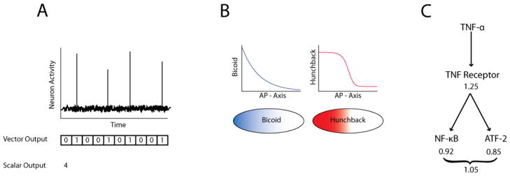
Neural activity consists of intermittent spikes known as action potentials. A series of spikes is known as a neural spike train. data spike train can be quantified as the total number of spikes over a given time period giving a scalar output. Alternatively, time can be divided into small time intervals such that the number of spikes occurring in each time interval is 1 or 0, enabling the spike train to be quantified as a binary vector output. As the total time frame is made longer, the vector becomes longer, and it becomes increasingly harder to adequately sample all possibilities in the entire vector space. (B) Bicoid and hunchback gradient in the Drosophila melanogaster embryo. In the developing embryo of Drosophila melanogaster, pre-deposited bicoid maternal mRNA is translated into a bicoid protein gradient along the anterior-posterior axis. Because bicoid is a cooperative transcriptional activator of hunchback, the smooth bicoid gradient leads to expression of hunchback in a much sharper concentration gradient which delineates the anterior and posterior halves of the embryo. (C) Schematic of the TNF signaling network. Individually, the capacities of the TNF-ATF-2 and the TNF-α NF-κB pathways are only ~0.9 bits of information. Combined, the network of pathways has only a marginally increased capacity of ~1.05 bits. Further investigation found that the capacity was limited at the receptor level at ~1.25 bits implying that the maximum capacity of the TNF network is ~1.25 bits regardless of the number of pathways or branch fidelity.

Fortunately, provided a sufficient amount of data, there are methods to estimate and correct for the bias [17]. One method [15] relies on the observation that the bias is a function of the sample size, and it tends toward zero as the sample size tends towards infinity. This relationship can be conveniently written as a series expansion with terms of inverse sample size:

$$I_{\text{biased}}=I_{\infty }+\frac{a_1}{N}+\frac{a_2}{N^2}+\cdots$$ [6]

where I_biased is the biased estimate of the mutual information, I_∞ is the estimate of the mutual information in the infinite sample size case, a_i (i = 1, 2, …) are coefficients that are particular to the signal and response distributions, and N is the total number of samples. For sufficiently large N, all terms above the first order are rendered negligible, and the biased estimate is linearly related to the inverse sample size. Furthermore, this linear relationship can be estimated by bootstrapping, i.e. by computing the mutual information on subsets of the data of different sizes. By plotting the biased estimate versus inverse sample size, fitting a line, and extrapolating to 1/N → 0 (corresponding to N → ∞), one can obtain an unbiased estimate of the mutual information.

Numerical computation of capacity

To calculate the capacity of a given system, a method is needed to determine the maximal value of the mutual information under all possible probability distributions of the signal, p(s), given the experimentally determined input-output relationship. At first, this may appear to be intractable; however, there are efficient algorithms to accomplish the task. These algorithms exist because mutual information is a smooth and strictly concave function of p(s). Hence, there is a single global maximum that can be identified by standard optimization methods akin to gradient ascent or by alternating maximization methods such as the easy-to-implement Blahut-Arimoto algorithm [9]. Additionally, the concave property allows the numerically determined solution to be independently verified, using the well-known Karush-Kuhn-Tucker conditions [9].

As part of these optimization routines, one can obtain not only the maximum value of the mutual information but also the signal distribution, p(s), that maximizes it. We caution, however, in attempting to interpret the biological significance of the maximizing signal distribution. Mutual information tends to be a non-steep function of the signal distribution and many signal distributions will yield mutual information close to the capacity. Hence, small fluctuations in the data, especially at the tails of the response distribution where sampling is the weakest, can change the specific distribution that yields the mathematical maximum without substantially affecting the capacity (maximum value) itself. Exploring and interpreting the space of signal distributions requires the use of constraints to compensate for small perturbations resulting from experimental noise, and their efficient numerical implementation is an active area of research [8, 18].

Applications of Information Theory in Biology

A major advantage of the information theoretic framework described above is that it can be easily implemented in a wide range of scenarios absent of any knowledge of the internal mechanisms or complexity of the system. The key to conducting such an analysis is to identify the boundaries of the communication channel and thus specify its input and output. As such, many applications of information theory to biology have been to characterize the information transmission capacity of specific signaling systems or network structures. One early example can be found in the application of information theory to the neural coding problem in neuroscience [19–21]. To acquire information about the outside world, a sensation is processed by a sensory organ into a stream of electrical impulses, called action potentials, which travel along a highway of neurons to the brain. The brain receives the neural signals and then proceeds to decode the information to recreate the original sensation. However, what is not immediately evident is how neurons encode such vivid depictions of the environment into a simple series of electrical pulses that can be decoded with remarkable fidelity.

One simple way to represent sensory information is to encode it into the rate of neuronal firing, which can be easily measured by counting the number of spikes within a timeframe and then averaging over time. Alternatively, information might be represented in the relative position of the spikes, referred to as a temporal coding scheme. As mentioned previously, experimentally measuring such a temporal code involves discretizing a time interval into bins and then assessing if a spike is present in each bin, designating a 1 to represent a full bin or 0 to indicate an empty one to generate a fixed length series of binary digits (figure 3A). This block of binary digits would then represent a code that a neuron would send. The capacity provides a way to evaluate rate coding, temporal coding, or any other hypothesized information coding mechanism based upon the ability to carry information. For example, information theory was used in the early analysis of neural codes to determine that temporal codes offer a greater potential to transmit information than simple rate codes [22].

Similar analyses can be used to evaluate how neural information transfer evolves over time. Since neural networks have the ability to learn, it may be possible for them to adapt to different sources of information. For example, the infomax principle [23], when applied to neurological sensing, posits that the brain can dynamically adjust to different inputs in order to maximize the amount of information provided by a sensory organ. Indeed, it has been shown that neural spikes display neural codes that adapt as the stimulus to the sensory organ changes to ensure that the amount of information transmitted is maximized [24, 25].

Another example of the importance of the fidelity of information transfer is found in the development of the embryo of the fruit fly, Drosphila melanogaster. In early developmental stages, the embryo consists of an undifferentiated collection of nuclei embedded in the common cytoplasm forming a so-called syncytium. Each nucleus must accurately determine its physical position within the embryo in order to adopt the appropriate developmental fate. To communicate information about position, a morphogen, a biochemical signal with a spatially graded distribution, typically encodes positional information via concentration. Any error in this process can lead to a fruit fly with body parts in the wrong locations or of the wrong sizes, which is often lethal.

Accuracy in the systems that communicate between the morphogen and fate decision processes is of paramount importance, thus we would expect to see sufficient information communicated from the morphogen to the molecular mechanisms involved in cell-decision making. For instance, a morphogen essential in patterning the anterior-posterior (A-P) embryonic axis is the bicoid transcription factor. Bicoid, in turn, induces expression of hunchback protein in a concentration dependent manner. Interestingly, bicoid concentration decreases steadily from the anterior to the posterior end of the embryo, whereas hunchback concentration falls off sharply in the middle of the embryo in a “switch-like” fashion (figure 3B). This observation has led to the hypothesis that bicoid concentration encodes positional information that is transmitted to hunchback, thereby enabling a cell to determine whether it is located in the anterior or posterior half of the embryo. Until recently however, it was unclear whether this long-standing hypothesis could withstand quantitative scrutiny, as gene expression in individual cells is an inherently noisy process [26], which along with other sources of cell-to-cell or embryo-to-embryo variability could interfere with transmission of the positional information. To examine the capacity of the bicoid-hunchback communication channel in the presence of such noise, Tkacik et al. [7] used data collected by Gregor et al. [14] that simultaneously quantified bicoid and hunchback concentrations throughout many embryos, yielding a sample of their joint distribution. From this data, Tkacik et al. estimated that the mutual information between bicoid and hunchback and found experimentally that there was 1.5 ± 0.2 bits of positional information transmitted. Because 1 bit is the minimum needed to perfectly specify the A-P boundary (a binary outcome), it was concluded that the capacity of the bicoid-hunchback channel was sufficient for each cell to accurately determine whether they are located in the front or back half of the embryo. These measurements have been recently extended to show that multiple morphogens in combination are sufficient for each cell to uniquely determine its location along the A-P axis [27].

Recently, we extended information theory concepts to analyzing biochemical signaling networks, whose information transfer capacities were previously generally unknown [8]. Among several model systems, we focused on the network activated by tumor necrosis factor (TNF), a well-characterized potent activator of the cellular inflammatory response. Similar to many other signaling networks, it is generally believed that the concentration of TNF encodes biologically relevant information, such as the magnitude of infectious danger, and that this information is transmitted through the network to downstream transcription factors, such as NF-κB or ATF-2 (figure 3C). By measuring the NF-κB and ATF-2 responses (e.g., nuclear concentration after 30 min. stimulus) of many individual cells to various concentrations of TNF, we determined that the capacities of TNF-α NF-κB and TNF-ATF-2 pathways were each only ~0.9 bits of information [8]. This was a surprising result since these pathways were believed to be able to accurately specify much more than binary outcomes.

We also considered the capacity of the network as a whole, i.e. the pathways in combination, finding that the capacity of signaling from TNF to NF-κB and ATF-2 simultaneously was only ~1.0 bit. Stated another way, knowing only the NF-κB or only the ATF-2 response yields at most ~0.9 bits of information about the TNF concentration, whereas knowing both the NF-κB and ATF-2 responses yields at most ~1.0 bit of information. The marginal increase from ~0.9 to ~1.0 bit was due to the overlap (dependency) between the NF-κB and ATF-2 pathways at the level of the TNF receptor. Further analysis indicated that the capacity of TNF signaling through the TNF receptor-level complex, i.e., very early in the signaling pathway, was already quite limiting, ~1.25 bits, and therefore constituted an early information bottleneck in the network. Since all pathways within the TNF network rely on the same receptor, the data processing inequality (see above) implies that the maximum capacity of the TNF network is ~1.25 bits regardless of the number of downstream pathways or their fidelity. Similar bottlenecks can constrain alternative strategies for improved information transmission, such as using negative feedback, temporal averaging, or multiple cells to combat noise which for TNF signaling yield capacities of at most ~1–2 bits [8].

Up to this point, we discussed how channel capacity can be used to measure the maximum information flow through a communications channel, but we made no assumption about the amount of information that may be needed to make adequate decisions. One way to approach this problem is to assume that the decision can be made based on imperfect information as long as the associated error can be tolerated by the system. To mathematically articulate this possibility and to quantitatively estimate how the information required is related to error tolerance, rate distortion theory, a major branch of information theory, can be utilized. More specifically, this theory provides an analytical framework to determine the minimum channel capacity required to transmit information at a given rate of error (distortion). This lower bound on the information needed is of interest as, presumably, it is less resource intensive and thus preferable to construct a channel with a lower capacity than would be available, in principle, given a perfect biochemical signaling network. Conveniently, biology provides many interesting situations where such distortion analysis can be undertaken and where it can yield useful results.

One example is provided by the remarkable chemotactic ability of the amoebae Dictyostelium discoideum, known more commonly as the slime mold. During its unicellular life cycle, D. discoideum cells feed upon bacteria until the supply is exhausted at which point the cells begin to starve and release the chemoattractant cyclic adenosine monophosphate (cAMP). Individual amoebae cells will then migrate up a concentration gradient of this chemoattractant and combine to form a large multicellular aggregate to cooperatively search for more food or form spores. It is evident that during aggregation each cell must be able to acquire information about the local cAMP concentration gradient, otherwise not enough cells would converge to form the aggregate. Additionally, the chemotaxis signaling system of D. discoideum exhibits directional biasing such that a cell is more inclined to maintain the same direction of motility, even after the local concentration gradient fluctuates. This result raises the question of whether a properly biased cell may require less information to accurately assess the concentration gradient than an unbiased one.

To address this question, Andrews et al. [28] used rate distortion theory in tandem with the local-excitation, global-inhibition (LEGI) chemotaxis model [29, 30] to construct a distortion constrained model of D. discoideum chemotaxis. By setting the distortion to be a function of the angle mismatch between cAMP gradient direction and cellular migration direction, the model demonstrated that cells whose directional movement bias becomes aligned with the direction of the gradient do indeed require less information than unbiased cells to migrate efficiently up the gradient. Furthermore, the study suggested that for unbiased cells the LEGI model achieved the lowest mutual information required for any given distortion. The relevance of this conclusion is that it suggests that the information of the gradient direction in the chemotaxis signaling network is the object of optimization presumably at the cost of cellular energy.

A common theme throughout the prior examples is that information can be thought of as a distinct quantity that cellular systems necessarily require for survival whether it is for describing the inflammatory cues surrounding a cell or morphogen gradients directing embryogenesis. The examined studies provide support for the premise that cells seek to acquire information sufficient only to ensure continued existence and that any additional capacity can be acquired but presumably at a higher energetic cost to the cell. By placing physical upper limits to the transfer of information in biological systems, information theory can direct a novel line of inquiry in well-established systems. For example, after discovering that the TNF-NF-κB signaling network holds a capacity of ~1 bit with information theory, we can now ask why such a system is limited to only a binary choice or where in the signaling pathway the bottleneck of information occurs. Similarly in the fruit fly D. melanogaster, we can quantify to what degree each molecular mechanism contributes to create such complex patterns of morphogen gradients that ultimately lead to the differentiation of the adult fruit fly.

Conclusion

Information theory provides suitable mathematical tools to rigorously evaluate models for how information is encoded, transmitted, and decoded in biological systems. In particular, channel capacity can measure the ability of a biological signaling system to transduce information and test hypotheses for how information is efficiently processed. Additionally, rate distortion theory can elucidate the tradeoff between error and performance to aid in the understanding of the design of biological systems. Here we emphasize again that the major strength of information theory is that initial analyses can be performed without detailed knowledge of the underlying complexity of the system, which provide useful insights into what a signaling process can or cannot achieve.

Signaling pathways and networks have evolved to inform the cell about changes in the environmental conditions, including the presence and current function of the neighboring cells. As a result, these networks are specialized in the processing and transmission of information in order to confine the decision space of phenotypic responses and to enable appropriate reactions to a dynamic environment. Many diseases, including multiple forms of cancer, may emerge and progress if this information processing capability is impaired or if information leads to an inappropriate match between environmental cues and such cell responses as proliferation and apoptosis. Thus, this information based analysis may provide a useful ground for discussion of how signaling and cell decision processes are controlled in health and disease, and how they can be affected by mainstream treatment modalities.

We envision that information theory will become as widespread in analyzing cell signaling systems as it is for analyzing man-made communications channels. With the hopes of encouraging more biologists to use information theory as a method of analysis, we have provided this brief primer and anticipate that further work in this field will aid in understanding how cells convey signals and process information effectively despite relying on often very imprecise molecular means to do so.

References

- 1.Perkins TJ, Swain PS. Strategies for cellular decision-making. Mol Syst Biol. 2009:5. doi: 10.1038/msb.2009.83. [DOI] [PMC free article] [PubMed] [Google Scholar]
- 2.Albeck JG, et al. Modeling a Snap-Action, Variable-Delay Switch Controlling Extrinsic Cell Death. PLoS Biol. 2008;6(12):e299. doi: 10.1371/journal.pbio.0060299. [DOI] [PMC free article] [PubMed] [Google Scholar]
- 3.Rosenfeld N, et al. Gene Regulation at the Single-Cell Level. Science. 2005;307(5717):1962–1965. doi: 10.1126/science.1106914. [DOI] [PubMed] [Google Scholar]
- 4.Borst A, Theunissen FE. Information theory and neural coding. Nat Neurosci. 1999;2(11):947–957. doi: 10.1038/14731. [DOI] [PubMed] [Google Scholar]
- 5.Tkacik G, Callan CG, Bialek W. Information capacity of genetic regulatory elements. Physical Review E. 2008;78(1):011910. doi: 10.1103/PhysRevE.78.011910. [DOI] [PMC free article] [PubMed] [Google Scholar]
- 6.Tkacik G, Walczak AM, Bialek W. Optimizing information flow in small genetic networks. Physical Review E. 2009;80(3):031920. doi: 10.1103/PhysRevE.80.031920. [DOI] [PMC free article] [PubMed] [Google Scholar]
- 7.Tkačik G, Callan CG, Bialek W. Information flow and optimization in transcriptional regulation. Proceedings of the National Academy of Sciences. 2008;105(34):12265–12270. doi: 10.1073/pnas.0806077105. [DOI] [PMC free article] [PubMed] [Google Scholar]
- 8.Cheong R, et al. Information Transduction Capacity of Noisy Biochemical Signaling Networks. Science. 2011;334(6054):354–358. doi: 10.1126/science.1204553. [DOI] [PMC free article] [PubMed] [Google Scholar]
- 9.Cover T, Thomas J. Elements of Information Theory. Wiley-Interscience; 1991. [Google Scholar]
- 10.Shannon CE. A mathematical theory of communication. Bell system technical journal. 1948:27. [Google Scholar]
- 11.Mian IS, Rose C. Communication theory and multicellular biology. Integrative Biology. 2011;3(4):350–367. doi: 10.1039/c0ib00117a. [DOI] [PubMed] [Google Scholar]
- 12.Waltermann C, Klipp E. Information theory based approaches to cellular signaling. Biochimica et Biophysica Acta (BBA) - General Subjects. 2011;1810(10):924–932. doi: 10.1016/j.bbagen.2011.07.009. [DOI] [PubMed] [Google Scholar]
- 13.Berger T. Living Information Theory. IEEE Information Theory Society Newsletter. 2003;53(1):1–19. [Google Scholar]
- 14.Gregor T, et al. Probing the Limits to Positional Information. Cell. 2007;130(1):153–164. doi: 10.1016/j.cell.2007.05.025. [DOI] [PMC free article] [PubMed] [Google Scholar]
- 15.Strong SP, et al. Entropy and Information in Neural Spike Trains. Physical Review Letters. 1998;80(1):197. [Google Scholar]
- 16.Kraskov A, Stögbauer H, Grassberger P. Estimating mutual information. Physical Review E. 2004;69(6):066138. doi: 10.1103/PhysRevE.69.066138. [DOI] [PubMed] [Google Scholar]
- 17.Panzeri S, et al. Correcting for the Sampling Bias Problem in Spike Train Information Measures. Journal of Neurophysiology. 2007;98(3):1064–1072. doi: 10.1152/jn.00559.2007. [DOI] [PubMed] [Google Scholar]
- 18.Bialek W, Setayeshgar S. Physical limits to biochemical signaling. Proceedings of the National Academy of Sciences of the United States of America. 2005;102(29):10040–10045. doi: 10.1073/pnas.0504321102. [DOI] [PMC free article] [PubMed] [Google Scholar]
- 19.MacKay DM, McCulloch WS. The Limiting Information Capacity of a Neuronal Link. Bulletin of Mathematical Biophysics. 1952;14:127–135. [Google Scholar]
- 20.Rapoport A, Horvath WJ. The theoretical channel capacity of a single neuron as determined by various coding systems. Information and Control. 1960;3(4):335–350. [Google Scholar]
- 21.Stein RB. The Information Capacity of Nerve Cells Using a Frequency Code. Biophysical Journal. 1967;7(6):797–826. doi: 10.1016/S0006-3495(67)86623-2. [DOI] [PMC free article] [PubMed] [Google Scholar]
- 22.Berry MJ, Warland DK, Meister M. The structure and precision of retinal spike trains. Proceedings of the National Academy of Sciences. 1997;94(10):5411–5416. doi: 10.1073/pnas.94.10.5411. [DOI] [PMC free article] [PubMed] [Google Scholar]
- 23.Linsker R. Perceptual Neural Organization: Some Approaches Based on Network Models and Information Theory. Annual Review of Neuroscience. 1990;13(1):257–281. doi: 10.1146/annurev.ne.13.030190.001353. [DOI] [PubMed] [Google Scholar]
- 24.Fairhall AL, et al. Efficiency and ambiguity in an adaptive neural code. Nature. 2001;412(6849):787–792. doi: 10.1038/35090500. [DOI] [PubMed] [Google Scholar]
- 25.Sharpee TO, et al. Adaptive filtering enhances information transmission in visual cortex. Nature. 2006;439(7079):936–942. doi: 10.1038/nature04519. [DOI] [PMC free article] [PubMed] [Google Scholar]
- 26.Elowitz MB, et al. Stochastic Gene Expression in a Single Cell. Science. 2002;297(5584):1183–1186. doi: 10.1126/science.1070919. [DOI] [PubMed] [Google Scholar]
- 27.Dubuis JO, et al. Positional information, in bits. 2011 doi: 10.1073/pnas.1315642110. arXiv.org:1201.0198 [q-bio.MN] [DOI] [PMC free article] [PubMed] [Google Scholar]
- 28.Andrews BW, Iglesias PA. An Information-Theoretic Characterization of the Optimal Gradient Sensing Response of Cells. PLoS Comput Biol. 2007;3(8):e153. doi: 10.1371/journal.pcbi.0030153. [DOI] [PMC free article] [PubMed] [Google Scholar]
- 29.Wang CJ, et al. Diverse Sensitivity Thresholds in Dynamic Signaling Responses by Social Amoebae. Sci Signal. 2012;5(213):ra17. doi: 10.1126/scisignal.2002449. [DOI] [PMC free article] [PubMed] [Google Scholar]
- 30.Levchenko A, Iglesias PA. Models of Eukaryotic Gradient Sensing: Application to Chemotaxis of Amoebae and Neutrophils. Biophysical Journal. 2002;82(1):50–63. doi: 10.1016/S0006-3495(02)75373-3. [DOI] [PMC free article] [PubMed] [Google Scholar]