A Simulation Environment for Diffusion Weighted MR Experiments in Complex Media

Abstract

Simulations of diffusion in neural tissues have traditionally been limited to analytical solutions, to grid-based solvers, or to small-scale Monte Carlo simulations. None of these approaches has had the capability to simulate realistic complex neural tissues on the scale of even a single voxel of reasonable (i.e. clinical) size. An approach is described that combines a Monte Carlo Brownian dynamics simulator capable of simulating diffusion in arbitrarily complex polygonal geometries with a signal integrator flexible enough to handle a variety of pulse sequences. Taken together, this package provides a complete and general simulation environment for diffusion MRI experiments. The simulator is validated against analytical solutions for unbounded diffusion and diffusion between parallel plates. Further results are shown for aligned fibers, varying packing density and permeability, and for crossing straight fibers.

Introduction

The sensitivity of MRI to the anisotropic diffusion of water within neural tissues provides some insight into the tissue structure. Spatial (diffusion tensor imaging, or DTI (1)) and spectral (q-space imaging (2)) variations of the diffusion weighted imaging (DWI) signal can be compared to the expected pulse signal response for simplified models of tissue structure. Analytical solutions are not available for structures with the complexity of real neural tissues, however.

An alternative approach is to simulate the DWI experiment numerically, including diffusion, tissue effects, and the influence of the pulse sequence. Much work has already been done in this area, with simulations ranging from grid-based finite difference methods to Monte Carlo Brownian dynamics to smoothed particle hydrodynamics (3–10), but most simulations are limited to simplified geometries. For example, (3) is limited to diffusion within a sphere and (5) simulates the one dimensional problem between two plates. The Camino package (8) provides general diffusion simulation capabilities, but relatively recent results (9) demonstrate random walks only in simplified domains. Furthermore, the type of Monte Carlo random walk implemented in Camino requires many time steps within the gradient pulse making simulations of the narrow pulse experiment difficult to achieve. Earlier related work by Frank and Rapp (10) allowed slightly more complex geometries, modeling diffusion within tubes along splines, but arbitrary geometries were not supported.

We have created a computational environment capable of simulating the entire DTI experiment by embedding MCell (11–13), a sophisticated Monte Carlo simulator for cellular microphysiology, within an MRI simulator that tracks particle location, state, and signal amplitude and phase, and whose output is connected to a suite of analysis and visualization tools. MCell supports models with arbitrarily complex geometry, multiple diffusion coefficients, particle interactions, and reactions at boundaries. MCell also has the capability to scale to very large problem sizes on parallel computers (11). Such features allow for simulations which can better approach the complexity of real neural tissues.

The combined simulation environment of MCell and our MR calculations is capable of modeling highly complex tissue structures, testing new pulse sequences, and developing new post-processing and analysis techniques. Here we demonstrate initial results validating the methods for unbounded diffusion and diffusion between parallel plates, and testing the effects of fiber permeability and packing density on fractional anisotropy (FA) for aligned cylindrical fibers.

Theory

Diffusion Weighted Imaging Simulation

For spins moving according to a time-dependent function x(t), the echo amplitude, E, generated by a standard spin echo or gradient echo sequence is given by the ensemble average of all the spins:

$$E=\langle e^{i\gamma {\int }_0^{TE}a\mathbf{G}(t)·\mathbf{x}(t)dt}\rangle .$$ (1)

In this equation γ is the gyromagnetic ratio; a is +1 for gradient echo sequences while for spin echo sequences it is +1 before and −1 after the 180° RF pulse; G(t) is the applied diffusion weighting vector; and x(t) is the spin position.

For standard spin echo experiments, ignoring ramp times and taking |G| to be constant during the diffusion encoding periods, Eq. 1 is often simplified to

$$E=\langle e^{-i\gamma \delta \mathbf{G}·({\overline{\mathbf{x}}}_2-{\overline{\mathbf{x}}}_1)}\rangle ,$$ (2)

where δ is the duration of the gradient pulse and x̄₁ and x̄₂ are the time-averaged positions of a given spin during the first and second diffusion encoding periods, respectively.

By simulating the diffusion of N_p individual spins with MCell, we can retain the generality of Eq. 1 by performing the integration numerically, similar to the approach of Szafer et al. (14):

$$E=\frac{1}{N_p}\sum _{j=1}^{N_p}{e}^{i\gamma {\sum }_{i=0}^{N_t}a\mathbf{G}(t_i)·{\mathbf{x}}_j(t_i)dt},$$ (3)

or

$$E=\frac{1}{N_p}\sum _{j=1}^{N_p}{e}^{i\gamma {\theta }_j},$$ (4)

where

$${\theta }_j=\sum _{i=0}^{N_t}a\mathbf{G}(t_i)·{\mathbf{x}}_j(t_i)dt,$$ (5)

and dt is the length of the time step used in the Monte Carlo simulation, N_t is the total number of time steps, and G and x are evaluated at each time step t_i.

Effects such as relaxation (including T₁, T₂, and wall relaxation) and magnetic susceptibility are not considered for the current work. Methods for dealing with such effects are known (14,15), and we believe that the flexibility of MCell and our simulation environment will allow us to add these features in future versions.

The user interface to our simulation, shown in Fig. 1, allows gradient directions which are defined by tessellating an icosahedron, as in (16,17). Users may specify the tessellation level from 1 to 5 (12 to 2562 gradient directions). The methods within the simulator itself support arbitrary gradient directions.

Figure 1.

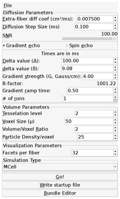
A view of the main user interface for the simulation environment.

Our current implementation can model both gradient echo and spin echo pulse sequences and the user interface allows users to specify all the parameters shown in Fig. 2, including the diffusion time, Δ, the gradient pulse duration, δ, and the gradient strength, G, as well as the gradient ramp time, t_r. The b-value is calculated automatically.

Figure 2.

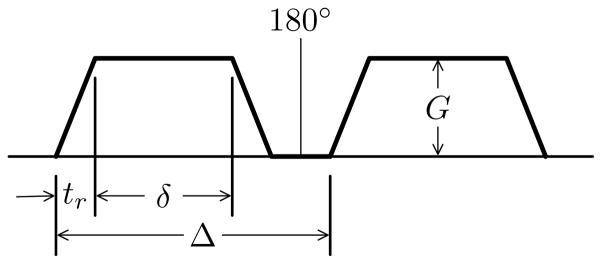
Parameters of the diffusion encoding pulse.

Simulating Diffusion by Monte Carlo Random Walk

Equation 3 allows us to calculate the signal given the diffusion gradient and spin locations. The spin locations are in turn computed by simulating particle diffusion. MCell (11–13) models diffusion of individual particles by a 3D Brownian dynamics random walk. Time is discretized into time steps of length dt. The location of each diffusing particle is updated every time step by a random displacement vector (or ray). If the ray traced by the diffusing particle intersects a boundary, the particle is reflected. If the particle’s path along the ray is unobstructed, the particle is placed at the endpoint of the ray until the next time step.

For each type of diffusing particle, random walk diffusion steps are scaled according to its associated diffusion coefficient, D. In MCell, diffusion steps are not of a fixed length, but are chosen to match the probability distribution for unbounded diffusion over the length of a single time step. In free space, the concentration, C, of particles is governed by the diffusion equation:

$$\frac{\partial C}{\partial t}=D{\nabla }^{2}C.$$ (6)

For a point source of M particles released at the origin at time t = 0, the solution only has a concentration gradient along the radial direction and can be given as

$$C(r,t)=\frac{M}{{(4\pi Dt)}^{3/2}}{e}^{-r^2/4Dt}$$ (7)

The fractional probability of finding a particle between r and r + dr at time t can then be given as

$$p_r(r,t)=\frac{4\pi r^{2}dr}{{(4\pi Dt)}^{3/2}}{e}^{-r^2/4Dt},$$ (8)

or, when defined in terms of the dimensionless parameter $s=r/\sqrt{4Dt}$,

$$p_r(s)=\frac{4}{\sqrt{\pi }}{s}^2{e}^{-s^2}ds.$$ (9)

This is the probability distribution used by MCell to choose diffusion step lengths for each particle.

The simplest random walk algorithms use a 3D Cartesian lattice, with particles confined to move a fixed distance along x, y, and z directions. Such methods are of limited utility for problems which have small features relative to the diffusion length scale, though, since the lattice size (and simulation time step) must be very small for accurate simulation of diffusion in the presence of small gaps and restrictions (12). Many lattice-free random walk algorithms, like that used in Camino, combine a fixed diffusion step length with random directions. Such methods do not reproduce the properties of free diffusion from time step to time step and thus require averaging over several time steps. Camino, for example, recommends a minimum of 50 time steps within the gradient block to achieve good averaging.

MCell allows for much longer simulation time steps—or many fewer time steps within the gradient block—by using Eq. 9 to initialize a look-up table containing a large number (1024 by default) of equally probably values of step length s. MCell stores another look-up table of equally probable radial directions (> 130, 000 directions by default). This set of radial directions is constructed with symmetry properties necessary to avoid directional bias. Then for each simulated time step, dt, a step length and radial direction are chosen at random from these look-up tables. The diffusion step is scaled by the appropriate factor ( $\sqrt{4Dt}$), and the ray describing the diffusing particle’s path for this time step is traced, reflecting elastically off any barriers in its path. Checking for intersections during ray tracing is the most computationally intense part of the simulation, but MCell uses a binning method, dividing the volume into spatial subvolumes, to limit the number of possible particle-surface interactions to check.

MCell is normally run as a stand-alone application, capable of recording system state at every time step. The complete state of the system at every time step is quite large, however. Since we only need to update the phase shift of each particle at each time step, we modified MCell to be a callable function from our simulation, calculating the contribution to the MRI signal at each time step.

Tissue Generation

Geometry is represented by polygonal surfaces of arbitrary detail and complexity. A polygonal surface is defined, as in the MCell model description language, by listing the locations of its vertices and the vertices for each face. A single triangle can be defined as follows:

triangle POLYGON_LIST {
 VERTEX_LIST {
    [0.0, 0.0, 0.0]
    [1.0, 0.0, 0.0]
    [0.0, 1.0, 0.0]
 }
 ELEMENT_CONNECTIONS {
    [0, 1, 2]
 }
}

Within our simulation, membrane permeability is modeled using MCell’s support for chemical reactions. A reaction rate may be assigned for all particles encountering a surface. Diffusing particles that hit a surface may undergo a reaction with a probability determined by the reaction rate for that particle and surface. Transport through the surface is one of several reactions supported by MCell. Particles transported through a boundary continue on their original path; particles that are not transported reflect elastically off the boundary. See Fig. 3. The diffusion coefficient for a particle is updated when it is transported, according to the type and orientation of the surface through which it was transported. We are able to create models with multiple diffusion coefficients in this way, having, e.g., distinct diffusion coefficients for the axonal core, myelin sheathing, and extraaxonal (bath) fluid.

Figure 3.

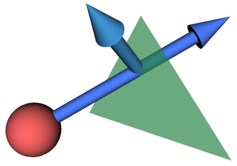
Diffusing particles encountering a boundary pass through or reflect elastically with a probability determined by a user-specified reaction rate.

Users may design tissues using the bundle editor interface, shown in Fig. 4, which allows users to specify multiple fiber bundles according to fiber radius, bundle radius, and number of fibers per bundle. Each bundle may also be curved along a spline.

Figure 4.

A snapshot of the bundle editor. A curved fiber bundle following a user designed spline crosses through the simulated volume (outer box) and measured voxel (inner box).

Users may also generate simple bundles of straight, aligned fibers with a specified orientation and packing density. These bundles can be arranged with regular hexagonal packing as in Fig. 5a or, for lower fiber densities, regions can be filled with randomly placed fibers with sizes varying around a mean radius as in Fig. 5b. For both packing strategies users specify two points describing the orientation of the bundle as well as the width and height of the bundle. For regular hexagonal packing, users also specify the fiber radius and the center-to-center spacing between fibers. For randomly packed fiber bundles, users specify the mean fiber radius, the standard deviation of the the fiber radii, the desired filling fraction, and the maximum number of attempts to place a fiber.

Figure 5.

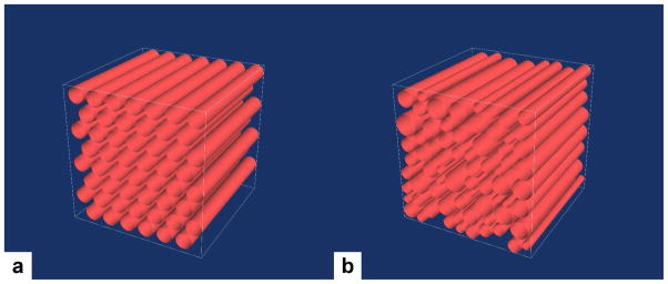
(a) A 200 μm³ voxel filled with hexagonally packed fibers with a radius of 12 μm. Volume fraction filled is 0.54. (b) A 200 μm³ voxel filled with randomly packed fibers with a mean radius of 12 μm and a standard deviation of 2 μm. Volume fraction filled is 0.57.

When randomly placing fibers, the location and radius of a new fiber are chosen and then intersections with previously placed fibers are checked. If an intersection is found, the fiber is discarded and another location and radius are chosen. If no intersection is found, the fiber is added to the collection of placed fibers and the total volume filled is incremented. This process continues until either the user-specified maximum number of attempts is reached or the filling fraction is exceeded.

In addition to long, straight fibers, we can also fill surrounding and interstitial spaces with randomly placed and oriented ellipsoidal cells with axis lengths randomly distributed around a given mean, as in Fig. 10. The user again specifies the mean radius and standard deviation as well as the total voxel filling fraction. The algorithm for the placement of ellipsoidal cells is similar to that for placing straight fibers, but intersection checking is simplified by checking intersections of bounding spheres rather than intersections among ellipsoids.

Figure 10.

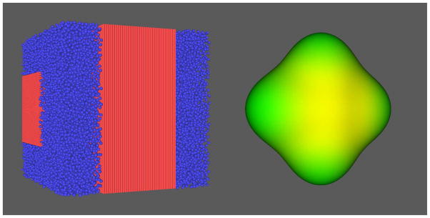
Crossing packed fibers surrounded by randomly oriented ellipsoidal cells (left) and the resulting q-ball orientation distribution function (right).

Users assign permeability to the generated surfaces and specify internal (core) and external (bath) diffusion coefficients. Though not supported directly by the user interface, the simulation environment allows for models with any number of diffusion coefficients, so it is also possible to construct models similar to the one described by Sen and Basser (18) with distinct diffusion coefficients for the axonal core, the myelin sheathing, and the extraaxonal bath materials.

Analysis and Visualization of Simulation Results

The simulation environment includes analysis tools for high angular resolution diffusion weighted MRI (17) to compute the spherical harmonic decomposition (SHD) and quantities derived from it, such as the the q-ball orientation distribution function (ODF) (19) according to the method described by Anderson (20). We have also developed a visualization package implemented with the Visualization Toolkit (VTK) (21). The visualization package displays the fibers simulated, the computed signal, the SHD, and the ODF. Output from the simulation is also compatible with other analysis packages, such as AFNI (22), which can be used to calculate derived quantities such as fractional anisotropy (FA) and mean diffusion (MD).

Results

The particle diffusion algorithms within MCell have been rigorously validated elsewhere (12, 13), but we will validate our signal calculation with two cases for which analytical solutions exist: unbounded diffusion and diffusion between parallel plates. In the case of unbounded diffusion, the signal decays exponentially,

$$E=e^{-bD},$$ (10)

where D is the diffusion coefficient and the b-value, b, is ${\gamma }^2{G}^2{\delta }^2(\mathrm{\Delta }-\frac{1}{3}\delta )$.

We simulated unbounded diffusion with δ = 1 μs, Δ = 10 ms, γ = 26752 rad/G s, D = 0.75 μm²/ms, and G varying linearly from 0 to 4.25 × 10⁵ G/cm, such that bD ranged from 0 to approximately 10. We ran simulations with 10⁴ to 10⁷ diffusing particles, using a simulation time step of length dt = 1 μs. The signal converged to the analytical solution as the number of diffusing particles increased, as shown in Fig. 6. The rate of convergence was slower than we had expected and requires further analysis, but we believe it is due to the difficulty of representing the tails of the distribution accurately with a finite number of particles.

Figure 6.

The signal E as a function of bD for various numbers of simulated particles: 10⁴ (gray circles), 10⁵ (black triangles), 10⁶ (gray squares), 10⁷ (black diamonds). Δ and δ are held constant, and G is varied to produce bD in a range from 0 to 10. The results converge toward the analytical solution, shown by the solid line, as the number of particles increases.

Next we simulated diffusion between parallel plates separated by a distance 2a. Again, an analytical solution is known for this case (15, 23). With a as defined here and for a gradient perpendicular to the plates, the signal in the large Δ limit is

$$E=\frac{2[1-cos(4\pi qa)]}{{(4\pi qa)}^2},$$ (11)

where q = γδG/(2π). We simulated qa in a range from 0 to 2, with a = 3 μm, γ = 26752 rad/G s, δ = 1 μs, and varying G. We simulated four different values of Δ. To reproduce the results shown by Callaghan (15), we similarly chose Δ as 0.2a²/D, 0.5a²/D, 1.0a²/D, and 2.0a²/D, with D = 0.75 μm²/ms as before. This resulted in values for Δ of 2.4 ms, 6.0 ms, 12.0 ms, and 24 ms. Note that for all cases, Δ is at least three orders of magnitude larger than δ, so the narrow pulse approximation is valid. As before, we used a simulation time step of length dt = 1 μs. The results for these simulations are shown in Fig. 7a. Again, we saw some dependence on the number of particles simulated, especially for higher values of qa and Δ. The data shown were generated using 10⁷ diffusing particles for Δ = 24 ms and 10⁶ particles for all other cases. The results match very well those shown by Callaghan (15).

Figure 7.

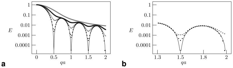
(a) The signal E as a function of qa for various values of Δ, defined in terms of a²/D, with Δ = 0.2a²/D (gray circles), Δ = 0.5a²/D (black triangles), Δ = a²/D (gray squares), and Δ = 2a²/D (black diamonds). The results converge toward the analytical solution for Δ → ∞, shown as a solid line. (b) The signal E as a function of qa for Δ = 2a²/D, simulated with 10⁶ particles (gray circles) and 10⁷ particles (black diamonds). Note that the simulation with 10⁷ particles more correctly tracks closer to the analytical solution for Δ → ∞.

The dependence of the signal on the number of particles simulated, N_p, is shown in Fig. 7b for Δ = 24 ms and N_p = 10⁶ and N_p = 10⁷. Divergence is especially pronounced at the high values of qa. It should be noted, however, that the solution is well resolved in the case where qa ≤ 1 and Δ ≤ a²/D (corresponding to a rather large b-value of (2π)²/D, or 52638 s/mm²) so clinically relevant simulations should converge well with fewer particles.

We have also simulated diffusion experiments with straight hexagonally packed cylindrical fibers. For all the following results, we used G = 4 G/cm, Δ = 77 ms, δ = 16 ms, and ramp times of 0.5 ms for a b-value of 2414 s/mm². We chose to keep the diffusion coefficient uniform with D = 0.75 μm²/ms and used a simulation time step of length dt = 0.1 ms. We generated straight fibers with radii of 1.2 μm. The signal was measured on a 100 μm³ voxel centered in a 200 μm³ simulated space, using 12 gradient directions oriented toward the vertices of a regular icosahedron. The motion of 10⁵ individual particles was simulated.

We tested the sensitivity of permeability changes with fibers packed to a density of 80%. Fiber permeability was varied by modifying the associated reaction rate on a logarithmic scale from 4.6 × 10⁻⁹ M⁻¹s⁻¹ to 2.2 × 10⁻⁸ M⁻¹s⁻¹. The calculated fractional anisotropy (FA) decreased as permeability increased, falling from a high of 0.90 for a reaction rate of 4.6 ×10⁻⁹ M⁻¹s⁻¹ to a low of 0.72 when the reaction rate was increased to 2.2 × 10⁻⁸ M⁻¹s⁻¹, as shown in Fig. 8.

Figure 8.

FA as a function of the reaction rate defining fiber permeability.

Next, keeping the fiber permeability fixed with a reaction rate of 1.0 × 10⁻⁹ M⁻¹s⁻¹, the fiber density was varied from 50% to 90% (near the maximum for hexagonally packed cylinders). The calculated FA increased with increasing fiber density, from 0.64 to 0.96, as shown in Fig. 9.

Figure 9.

FA as a function of fiber packing density.

We also simulated crossing fiber bundles, with fiber bundles placed perpendicular to one another and filling 80% of the voxel volume, with both bundles filling equal volume fractions of the voxel. The surrounding space was filled with randomly oriented ellipsoidal cells with an average diameter of 2.0 μm. Permeability of all the surfaces was kept fixed with a reaction rate set to 1.0×10⁻⁹ M⁻¹s⁻¹. We kept Δ = 77 ms, δ = 16 ms, and ramp times of 0.5 ms, but we increased the gradient strength to G = 6 G/cm to differentiate the fiber directions more clearly. The fibers and cells for this simulation are shown next to the resulting q-ball orientation distribution function (ODF) (19) in Fig. 10. The ODF was derived from the spherical harmonic decomposition (17) following the method described by Anderson (20).

As mentioned previously, the Camino package (8) provides somewhat similar functionality to the tools presented here. For comparison, we ran some simpler simulations using both our tools and the Camino package. We simulated a spin echo sequence on a hexagonal array of cylinders of radius 1.0 μm, with centers spaced 3.0 μm apart using 10⁴ diffusing particles. We used G = 4 G/cm, Δ = 77 ms, δ = 16 ms. Since the Camino package did not appear to support gradient ramp times, we set the ramp time to zero in our simulation. Surface permeability was also disabled for simplicity. The b-value for these simulations was 2100 s/mm². We simulated 930 time steps of length dt = 0.1 ms. Despite using MCell’s more realistic Monte Carlo random walk, which is essentially free of spatial granularity at each time step, our simulator ran this test case in 59 seconds, compared to 108 seconds for Camino. We attribute this difference largely to the highly optimized performance of MCell. In many cases an even larger performance difference can be expected. Recall that in the parallel plate simulation described earlier, only a single time step was required for the narrow pulse. Performing a similar experiment with Camino would require significantly smaller time steps—a minimum of 50 time steps for the gradient pulse is suggested—and thus would require an additional 50 times more simulation time.

Discussion

Our software allows researchers to simulate various MRI experiments (pulse sequences, gradient directions, b-values, etc.) and to understand better what features will can be detected before any MRI scans are even done. As a tool in experiment design, then, our software could be useful in finding the most cost-effective MRI prescription capable of detecting changes of interest to a study.

The constructed geometry used in this initial demonstration is fairly simplistic, with straight, densely packed fibers, but the ability to vary packing density, fiber permeability, and both interior and exterior diffusion coefficients allows us to test a wide range of realistic models. The underlying support for complex geometries is quite flexible, and future work will include more realistic large scale models.

It is also interesting to consider whether Monte Carlo methods such as these could reproduce analytical solutions for infinite time solutions, like those found in Sen and Basser (18). Whether a reasonable estimate of the infinite time solution can be simulated in finite time depends on the stiffness of the problem, i.e. the difference in diffusion time scales associated with the various simulated materials.

Our simulation environment is capable of modeling several structural sources of anisotropy in white matter, including variations in diffusion coefficients, particle concentrations, and membrane permeabilities. Beaulieu (24) provides a comprehensive review of these sources of anisotropy and discusses several models of pathology that we believe are amenable to testing within our framework, such as demyelination and membrane degradation. In addition, other modes of water motion present in white matter, such as active transport due to molecular water pumps (25), should also be tractable with our simulation tools, and will be a focus of future work.

Precise values for diffusion coefficients and membrane permeabilities are difficult to measure—diffusion coefficients themselves are often calculated by the same techniques which we are simulating here—and generating meshes representing true fiber dimensions from histology is a painstaking process, so perfect realism in our simulations may be too much to expect. We can, however, determine the degree to which the MRI signal is sensitive to changes in various model parameters. In addition, our software provides a unique platform for testing analysis methods in an environment where the underlying geometry and fiber properties are known a priori.

We are in the process of adding a more flexible model for pulse sequence specification to support other types of sequences (e.g. hyperecho sequences). Because we are able to model different compartments, the mechanisms to include T₁, T₂, and magnetic susceptibility are possible, and due to MCell’s explicit support for boundary interactions, mechanisms to model wall relaxation are also possible. Implementing and testing those mechanisms is beyond the scope of the current paper, but we will address those issues separately in future work. Finally, we are extending the scale of possible models by using a parallelized version of MCell (11), allowing us to simulate much larger geometries. While our work has focused on applications related to human brain imaging, the tools developed here could be found useful in other areas of research, such as diffusion in porous media.

Conclusion

We have presented a flexible MR simulation environment based on a Monte Carlo diffusion simulation package specifically designed for the complexities of microcellular physiology. Users are able to simulate MR diffusion experiments with realistic pulse sequences and arbitrarily complex geometry. We have validated the environment against known analytical solutions—unbounded diffusion and diffusion between parallel plates—and also shown results for fractional anisotropy as a function of membrane permeability and fiber packing density.

List of Symbols

E

echo amplitude

t

time

γ

gyromagnetic ratio

a

sign (+1 or −1)

G

gradient

x

spin position

θ_j

phase of particle j

Δ

diffusion time

δ

gradient pulse duration

t_r

ramp time

b

b value

x̄

time-averaged spin position

N_p

number of diffusing particles

N_t

number of time steps

C

particle concentration

D

diffusion coefficient

r

radius

s

dimensionless diffusion length parameter

p_r

probability of finding a particle at radius r

i

imaginary unit

e

Euler’s number or Napier’s constant

π

pi

μ

mu

∇

nabla

References

- 1.Basser PJ, Mattiello J, LeBihan D. Estimation of the effective self-diffusion tensor from the NMR spin echo. J Magn Reson. 1994;103:247–254. doi: 10.1006/jmrb.1994.1037. [DOI] [PubMed] [Google Scholar]
- 2.Callaghan P. Principles of NMR Microscopy. Oxford: 1993. [Google Scholar]
- 3.Kuchel PW, Lennon AJ, Durrant C. Analytical solutions and simulations for spin echo measurements of diffusion of spins in a sphere with surface and bulk relaxation. J Magn Reson B. 1996;112:1–17. doi: 10.1006/jmrb.1996.0103. [DOI] [PubMed] [Google Scholar]
- 4.Stanisz GJ, Wright GA, Henkelman RM, Szafer A. An analytical model of restricted diffusion in bovine optic nerve. Magnetic Resonance in Medicine. 1997;37:103–111. doi: 10.1002/mrm.1910370115. [DOI] [PubMed] [Google Scholar]
- 5.Duh A, Mohoric A, Stepisnik J. Computer simulation of the spin echo spatial distribution in the case of restricted self diffusion. J Magn Reson. 2001;148:257–266. doi: 10.1006/jmre.2000.2257. [DOI] [PubMed] [Google Scholar]
- 6.Meier C, Dreher W, Leibfritz D. Diffusion in compartmental systems. I. A comparison of an analytical model with simulations. Magnetic Resonance in Medicine. 2003;50:500–509. doi: 10.1002/mrm.10557. [DOI] [PubMed] [Google Scholar]
- 7.Hwang SN, Chin CL, Wehrli FW, Hackney DB. An image-based finite difference model for simulating restricted diffusion. Magnetic Resonance in Medicine. 2003;50(2):373–382. doi: 10.1002/mrm.10536. [DOI] [PubMed] [Google Scholar]
- 8.Cook PA, Bai Y, Nedjati-Gilani S, Seunarine KK, Hall MG, Parker GJ, Alexander DC. Camino: Open-Source Diffusion-MRI Reconstruction and Processing. Proc. ISMRM 14th Scientific Meeting; Seattle, WA: International Society of Magnetic Resonance in Medicine; 2006. p. 2759. [Google Scholar]
- 9.Hall MG, Alexander DC. Finite pulse widths improve fibre orientation estimates in diffusion tensor MRI. Proc. ISMRM 14th Scientific Meeting; Seattle, WA: International Society of Magnetic Resonance in Medicine; 2006. p. 1076. [Google Scholar]
- 10.Frank LR, Rapp JL. Smoothed particle hydrodynamic (SPH) simulation of diffusion in realistic neural tissue models. Proc. ISMRM 13th Scientific Meeting; Miami, FL: International Society of Magnetic Resonance in Medicine; 2005. p. 839. [Google Scholar]
- 11.Balls GT, Baden SB, Kispersky T, Bartol TM, Sejnowski TJ. A Large Scale Monte Carlo Simulator for Cellular Microphysiology. ipdps. 2004;01:42a. [Google Scholar]
- 12.Stiles JR, Bartol TM. Monte Carlo methods for simulating realistic synaptic microphysiology using MCell. In: Schutter ED, editor. Computational Neuroscience: Realistic Modeling for Experimentalists. CRC Press; 2001. pp. 87–127. [Google Scholar]
- 13.Stiles JR, Van Helden D, Bartol TM, Salpeter EE, Salpeter MM. Miniature endplate current rise times < 100 μs from improved dual recordings can be modeled with passive acetylcholine diffusion from a synaptic vesicle. Proceedings of the National Academy of Sciences of the United States of America. 1996;93:5747–5752. doi: 10.1073/pnas.93.12.5747. [DOI] [PMC free article] [PubMed] [Google Scholar]
- 14.Szafer A, Zhong J, Gore JC. Theoretical Model for Water Diffusion in Tissues. Magnetic Resonance in Medicine. 1995;33(5):697–712. doi: 10.1002/mrm.1910330516. [DOI] [PubMed] [Google Scholar]
- 15.Callaghan PT. Pulsed-Gradient Spin-Echo NMR for Planar, Cylindrical, and Spherical Pores under Conditions of Wall Relaxation. J Magn Reson. 1995 Mar;113(1):53–59. [Google Scholar]
- 16.Frank LR. Anisotropy in high angular resolution diffusion weighted MRI. Magn Reson Med. 2001 Jun;45(6):935–939. doi: 10.1002/mrm.1125. [DOI] [PubMed] [Google Scholar]
- 17.Frank LR. Characterization of anisotropy in high angular resolution diffusion weighted MRI. Magn Reson Med. 2002 Jun;47(6):1083–1099. doi: 10.1002/mrm.10156. [DOI] [PubMed] [Google Scholar]
- 18.Sen PN, Basser PJ. A model for diffusion in white matter in the brain. Biophysical Journal. 2005 Nov;89:2927–2938. doi: 10.1529/biophysj.105.063016. [DOI] [PMC free article] [PubMed] [Google Scholar]
- 19.Tuch DS, Reese TG, Wiegell MR, Wedeen VJ. Diffusion MRI of complex neural architecture. Neuron. 2003;40:885–895. doi: 10.1016/s0896-6273(03)00758-x. [DOI] [PubMed] [Google Scholar]
- 20.Anderson AW. Measurement of Fiber Orientation Distributions Using High Angular Resolution Diffusion Imaging. Magnetic Resonance in Medicine. 2005;54:1194–1206. doi: 10.1002/mrm.20667. [DOI] [PubMed] [Google Scholar]
- 21.Schroeder W, Martin K, Lorensen B. Visualization Toolkit: An Object-Oriented Approach to 3D Graphics. 4. Kitware, Inc; 2006. [Google Scholar]
- 22.Cox RW. AFNI: Software for analysis and visualization of functional magnetic resonance neuroimages. Computers and Biomedical Research. 1996;29:162–173. doi: 10.1006/cbmr.1996.0014. [DOI] [PubMed] [Google Scholar]
- 23.Tanner JE, Stejskal EO. Restricted Self-Diffusion of Protons in Colloidal Systems by the Pulsed-Gradient, Spin-Echo Method. J Chem Phys. 1968 Aug;49(4):1768–1777. [Google Scholar]
- 24.Beaulieu C. The basis of anisotropic water diffusion in the nervous system - a technical review. NMR in Biomedicine. 2002;15:435–455. doi: 10.1002/nbm.782. [DOI] [PubMed] [Google Scholar]
- 25.Baslow MH. Evidence supporting a role for N-acetyle-L-aspartate as a molecular water pump in myelinated neuon in the central nervous system: An analytical review. Neurochemistry International. 2002;40:295–300. doi: 10.1016/s0197-0186(01)00095-x. [DOI] [PubMed] [Google Scholar]