Comparing methods for estimating R₀ from the size distribution of subcritical transmission chains

Abstract

Many diseases exhibit subcritical transmission (i.e. 0 < R₀ < 1) so that infections occur as self-limited ‘stuttering chains’. Given an ensemble of stuttering chains, information about the number of cases in each chain can be used to infer R₀, which is of crucial importance for monitoring the risk that a disease will emerge to establish endemic circulation. However, the challenge of imperfect case detection has led authors to adopt a variety of work-around measures when inferring R₀, such as discarding data on isolated cases or aggregating intermediate-sized chains together. Each of these methods has the potential to introduce bias, but a quantitative comparison of these approaches has not been reported. By adapting a model based on a negative binomial offspring distribution that permits a variable degree of transmission heterogeneity, we present a unified analysis of existing R₀ estimation methods. Simulation studies show that the degree of transmission heterogeneity, when improperly modeled, can significantly impact the bias of R₀ estimation methods designed for imperfect observation. These studies also highlight the importance of isolated cases in assessing whether an estimation technique is consistent with observed data. Analysis of data from measles outbreaks shows that likelihood scores are highest for models that allow a flexible degree of transmission heterogeneity. Aggregating intermediate sized chains often has similar performance to analyzing a complete chain size distribution. However, truncating isolated cases is beneficial only when surveillance systems clearly favor full observation of large chains but not small chains. Meanwhile, if data on the type and proportion of cases that are unobserved were known, we demonstrate that maximum likelihood inference of R₀ could be adjusted accordingly. This motivates the need for future empirical and theoretical work to quantify observation error and incorporate relevant mechanisms into stuttering chain models used to estimate transmission parameters.

1. Introduction

For many emerging or potentially re-emerging diseases, outbreaks occur as isolated pockets of infection because relatively weak transmissibility prevents epidemic spread. In these circumstances, continual presence of disease requires introduction of a primary infection by spillover from a non-human reservoir or by geographic importation. Once a primary infection is present, any subsequent secondary transmission results in a ‘stuttering chain’ of transmission that eventually dies out because transmissibility is relatively weak. This subcritical transmission is a defining characteristic of stage III zoonoses, such as monkeypox, Nipah virus, H5N1 avian influenza, and Leishmania in-fantum (Taylor et al., 2001; Woolhouse and Gowtage-Sequeria, 2005; Wolfe et al., 2007; Lloyd-Smith et al., 2009). Subcritical transmission is also seen with vaccine preventable diseases such as measles and polio when local vaccination coverage is sufficiently high (Jansen et al., 2003; King et al., 2004; Gay et al., 2004; O’Reilly et al., 2012; Minor, 2012).

The exact conditions under which all chains go extinct can be described in terms of the reproductive number, R₀, which is the average number of cases caused by a typical infected individual. All transmission chains will be self-limited when 0 < R₀ < 1. (For simplicity of presentation, we will use the symbol R₀ to represent all reproductive numbers in this study, although this symbol is often reserved for the basic reproductive number associated with a fully susceptible population.)

Although subcritical transmission is ubiquitous, study of its dynamics has recently been highlighted as a gap in the modeling literature (Lloyd-Smith et al., 2009). In particular, robust inference of R₀ from stuttering chain data is of crucial importance for determining whether a disease is close to the R₀ = 1 threshold that would permit epidemic or endemic spread. Knowledge of R₀ also indicates the relative burden of primary infections versus secondary transmission (De Serres et al., 2000). In addition, monitoring how R₀ changes through time can help to identify shifts in transmissibility owing to environmental or evolutionary change, and hence to elucidate the ecological and evolutionary drivers of disease emergence (Pepin et al., 2010; Antia et al., 2003; Arinaminpathy and McLean, 2009).

The larger the reproductive number, the more secondary transmission will occur and so stuttering chains are expected to contain more cases. Since secondary transmission is stochastic in nature, R₀ cannot be inferred from the number of cases in a single chain. However the distribution of chain sizes contains enough information to infer transmission parameters (De Serres et al., 2000; Jansen et al., 2003; Farrington et al., 2003; Ferguson et al., 2004; Blumberg and Lloyd-Smith, 2013). If there is a large amount of data with no observation errors, then estimation of R₀ from chain size data is straightforward. In this case the maximum likelihood (ML) value for the reproductive number is ${\widehat{R}}_0=1-\frac{1}{\overline{\mu }}$, a simple function of the observed average chain size, μ̄ (De Serres et al., 2000). However, there are many issues that interfere with this ideal result. One complicating factor, exemplified by surveillance data for human monkeypox (Rimoin et al., 2010; Jezek and Fenner, 1988), is that data are often sparse and imperfect, owing to logistical challenges in conducting surveillance because many of these diseases occur in remote places where poor health infrastructure impedes reliable reporting. Therefore, in many settings the observed chain size distribution will suffer from an unknown amount of observation error. A second complicating factor is that transmission heterogeneity may impact the observed chain size distribution, because the existence of super-spreaders causes chains to be small in most cases and very large in a few others (Lloyd-Smith et al., 2005; Garske and Rhodes, 2008; Nishiura et al., 2012; Blumberg and Lloyd-Smith, 2013). If heterogeneity is not properly accounted for, studies may be inclined to ignore isolated cases as ‘unreliable data’ because of discrepancy with model predictions. Because of the inter-relationship between the true chain size distribution, the observed distribution, and transmission parameters, different estimation approaches are likely to infer different values for R₀ and associated confidence intervals.

A number of different methods have been published that use the size distribution of stuttering transmission chains to infer R₀. A unifying theme of these approaches is that they frame stuttering chain transmission in terms of a branching process (Becker, 1974, 1977; Ball et al., 2002; Harris, 2002; Lange, 2010). In this framework, transmission is completely described by an ‘offspring distribution’ that gives the probability that an infected case will transmit infection to any given number of secondary cases. Many authors choose to use an offspring distribution that makes implicit assumptions about the amount of transmission heterogeneity. Some studies, particularly those inspired by SIR-type models that assume constant rates of transmission, recovery and death, specify that the offspring distribution is described by a geometric distribution (Ferguson et al., 2004; Farrington et al., 2003; Jansen et al., 2003). Other studies assume that the offspring distribution is described by the more homogeneous Poisson distribution (De Serres et al., 2000; Gay et al., 2004; Farrington et al., 2003; King et al., 2004). However, it has been found that the negative binomial distribution is a more versatile choice, because it can describe a flexible degree of transmission heterogeneity and can fit data from a range of infectious diseases (Lloyd-Smith et al., 2005).

The negative binomial distribution has two parameters: R₀ and the dispersion parameter, k. While R₀ represents the average reproductive number for the population as a whole, the dispersion parameter specifies how much variation there may be in individual levels of infectiousness. Since the variance of the negative binomial distribution is $R_0(1+\frac{R_0}{k})$, there is a high degree of individual variation in infectiousness when k is less than one. When k = 1 the negative binomial simplifies to a geometric distribution, and when k → ∞ it reduces to a Poisson distribution. It is possible to let k be a free parameter that is estimated jointly with R₀ from chain size data (Blumberg and Lloyd-Smith, 2013). Thus the use of a negative binomial offspring distribution provides a general framework to compare previously published methods that use chain size data to estimate R₀ for subcritical transmission.

Chain size analysis methods also differ in their approach to dealing with the aforementioned challenges of modeling imperfectly observed stuttering chain data. A specific point of contrast is that past inference methods differ in the relative importance they attribute to isolated cases. Several studies exclude isolated cases from their analysis as they fear these cases may be less likely to be observed than those in larger transmission chains, or that isolated cases may be more prone to false-positive error (Gay et al., 2004; King et al., 2004; De Serres et al., 2000). In contrast, other approaches aggregate intermediate chain sizes on the basis that the most important characteristics of the chain size distribution are the number of isolated cases and the size of the largest chain (Ferguson et al., 2004).

The quantitative impact on R₀ estimation arising from these different assumptions and work-around measures has not been studied. Here, we present a unified analysis where we compare all the methodological variants mentioned above. We first compare the results of applying these methods to measles data collected in the United States and Canada. As previous analyses have noted, we show that several models are unable to match the observed number of isolated cases. We find that this mismatch can be alleviated by the use of a negative binomial offspring distribution, but the impact of imperfect case detection remains a concern. Therefore, we explore how imperfect case detection affects the bias of R₀ estimation, by considering two existing models for how observation error arises (Ferguson et al., 2004). One observation model assumes that every case has the same independent probability of being observed, while the other model assumes that cases in large chains are more likely to be observed than isolated cases. In order to reconcile an apparent conflict between allowing a flexible degree of transmission heterogeneity and compensating for imperfect observation, we also show that it is possible to formulate a likelihood function that incorporates both of these concerns. Because this framework requires quantitative knowledge about the observation process, we identify a need for new techniques that characterize imperfect surveillance so that estimation of R₀ can be adjusted accordingly.

2. Methods

We use the term ‘chain’ to describe a primary infection and all secondary cases linked to it by one or more generations of transmission. This is sometimes called a ‘cluster’, ‘outbreak’ or ‘minor outbreak’ by other authors. We consider a ‘cluster’ to be a spatio-temporal aggregation of cases, which may contain overlapping chains (as sometimes observed in the field).

2.1. Data

We analyze measles data from the United States and Canada. The case ascertainment for measles is relatively strong because its symptoms are distinctive, reported cases were thoroughly investigated and effort was made to trace the transmission of each case so that the size of stuttering chains could be accurately determined (Gay et al., 2004; King et al., 2004). However, the possibility of missed cases is a valid concern (Harpaz et al., 2004).

The United States data consist of all confirmed measles cases reported to the Centers for Disease Control and Prevention for 1997–1999 (Gay et al., 2004). The Canadian data consist of the confirmed measles cases collected by the Notifiable Disease Reporting System and enhanced measles surveillance system from 1998–2001 (King et al., 2004). The United States data set consists of 336 cases distributed among 165 infection clusters, while the Canadian data set consists of 274 cases distributed among 49 clusters (table 1).

Table 1. Distribution of transmission chain sizes for measles.

Chain size	Number of chains United States (’97–’99)	Number of chains Canada (’98–’01)
1	122	35
2	13	5
3	10	3
4	6	1
5	5	0
6	2	1
8	2	1
9	1	0
11	1	0
13	1	0
15	1	0
17	0	1
30	0	1
33	1	0
155	0	1

With one exception of a United States cluster of size six which had two primary cases (that we count here as a chain of size six), all clusters were reported to contain just one primary infection due to geographic importation. However, the imported case was explicitly identified in only 64% of the United States clusters and 73% of the Canadian clusters, indicating that some cases were missed by surveillance. Keeping these limitations in mind, we treat each cluster as a single transmission chain.

2.2. Simulations

2.2.1. Model assumptions

Following convention for branching process models of transmission dynamics, we assume that the number of infections caused by each case is independent and identically distributed. Then a single offspring distribution describes the probabilities that a given case will cause any number of infections.

2.2.2. Simulations

Transmission chains were simulated by first choosing the number of offspring for the chain’s lone primary case according to the offspring distribution. Then, if the primary case generates secondary cases, the offspring of each secondary case is drawn randomly from the same offspring distribution. This routine is repeated for all successive secondary cases and the chain size is determined by the total number of cases that have arisen before the chain goes extinct. Every chain eventually goes extinct because all our simulations have R₀ < 1.

For most simulations, a negative binomial offspring distribution was used to model the offspring distribution (Lloyd-Smith et al., 2005; Garske and Rhodes, 2008; Nishiura et al., 2012; Blumberg and Lloyd-Smith, 2013). However, for simulations based on a Weibull-Poisson offspring distribution, which corresponds to a Weibull distributed infectious period (Lu and Shi, 2012). To implement this scenario, a normalized infectious period was first chosen according to a Weibull distribution with mean one. Then the number of offspring was chosen according to a Poisson distribution with a mean equal to R₀ times the chosen infectious period.

To investigate the impact of imperfect observation, each simulated chain was re-evaluated according to one of two possible observation models (Ferguson et al., 2004). In the ‘independent’ observation model, each case is observed with an independent probability p. In the ‘size-dependent’ observation model, each case has an independent probability of being a ‘sentinel’ case. Then, if a chain contains at least one sentinel case, all cases in the chain are observed (representing retrospective and prospective investigation). Otherwise no cases in the chain are observed. For both models, the observed chain size distribution is conditioned on chains containing at least one observed case (i.e. one cannot observe chains that have no observed cases).

2.3. Chain size statistics

2.3.1. Chain size distribution for perfect observation

Branching process theory provides a link between the offspring distribution and the chain size distribution (Dwass, 1969; Becker, 1974). Specifically, for a negative binomial offspring distribution, the probability, r_j, of a transmission chain having overall size j is given by (Nishiura et al., 2012; Blumberg and Lloyd-Smith, 2013),

$$r_j=\frac{\mathrm{\Gamma }(\mathit{kj}+j-1)}{\mathrm{\Gamma }\left(\mathit{kj}\right)\mathrm{\Gamma }(j+1)}\frac{{\left(\frac{R_0}{k}\right)}^{j-1}}{{(1+\frac{R_0}{k})}^{\mathit{kj}+j-1}}.$$ (1)

This formula is valid for R₀ < 1 and R₀ > 1, but in the case of R₀ > 1 the sum of the probabilities does not equal one because some chains may escape extinction.

When R₀ < 1 and all cases are observed, the average size of a transmission chain, μ, can be derived by noting that the expected number of cases in each generation follows a geometric series (De Serres et al., 2000):

$$\mu =1+R_0+R_0^2+\dots =\frac{1}{1-R_0}.$$ (2)

2.3.2. Observed chain size distribution for independent observation error

In our first model of imperfect detection we assume that each case has an independent probability p_ind of being detected. Then the probability, $s_j^{\prime }$, of observing j cases in an arbitrary stuttering chain becomes

$$s_j^{\prime }={\displaystyle \sum }_{k=j}^{\infty }{r}_k·\left(\begin{array}{c}k\\ j\end{array}\right)·p_{\mathit{\text{ind}}}^j·{(1-p_{\mathit{\text{ind}}})}^{k-j}.$$ (3)

Here the sum is over the possible range of true chain sizes for which j cases can be observed. The quantity within the summation is the joint probability that the true number of cases in a stuttering chain is k and that j of the k cases are actually observed. The overall probability, $r_j^{\prime }$, that a chain has an observed size j differs from $s_j^{\prime }$ since a normalization factor is needed to account for the probability that some chains will not be observed at all. Thus,

$$r_j^{\prime }=\frac{s_j^{\prime }}{1-s_0^{\prime }}.$$ (4)

Under the assumption of independently observed cases, the overall probability, p_obs, of observing a randomly chosen case is equal to p_ind.

2.3.3. Observed chain size distribution for size-dependent observation error

In our second model of imperfect detection we assume that each case has an independent probability p_sent of being a sentinel case that guarantees all cases in the chain will be observed. The probability, v_j that a chain of true size j is unobserved is,

$$v_j={(1-p_{\mathit{\text{sent}}})}^j.$$

Thus the probability, $s_0^{\prime }$, that a randomly chosen chain is unobserved is,

$$s_0^{\prime }={\displaystyle \sum }_{k=1}^{\infty }{r}_k·v_k.$$

The overall probability that a chain has an observed size of j is the probability of a chain having true size j times the probability it includes at least one sentinel case, normalized by the probability that the chain is observed at all. Accordingly,

$$r_j^{\prime }=\frac{r_j·(1-v_j)}{1-s_0^{\prime }}.$$ (5)

Under the assumption of size-dependent chain observation, the overall probability p_obs of seeing a randomly chosen case is greater than p_sent, because non-sentinel cases can be observed. The overall probability can be calculated by properly normalizing the proportion of chains that are observed according to,

$$p_{\mathit{\text{obs}}}=\frac{{{\displaystyle \sum }}_{j=1}^{\infty }j·r_j·(1-v_j)}{\mu }.$$ (6)

Unfortunately this relationship cannot be easily inverted to obtain a closed form relationship between p_obs and p_sent. However, the relationship between these variables can be determined numerically for a given pair of R₀ and k values.

2.3.4. Observed average chain size

The expected value for the observed average chain size, μ^*, can be computed by making an explicit calculation, or equivalently by making a correction to p_obs · μ to account for some chains being unobserved. Specifically,

$${\mu }^{\ast }={\displaystyle \sum }_{j-1}^{\infty }j·r_j^{\prime }=\frac{p_{\mathit{\text{obs}}}·\mu }{1-s_0^{\prime }}.$$ (7)

In the case of independent observation error, p_ind · μ < μ^* < μ, because although some cases are unobserved, μ^* is biased upwards relative to p_ind · μ since some chains are completely unobserved. In the case of size-dependent observation, μ^* > μ because larger chains are more likely to be observed than smaller ones.

The observed average size of all chains for which at least two cases were observed (i.e. at least one secondary infection occurred) is

$${\mu }_s^{\ast }=\frac{{\mu }^{\ast }-r_1^{\prime }}{1-r_1^{\prime }}.$$ (8)

2.4. Maximum likelihood inference

When we treat data at face value and ignore the complications of imperfect observation, the likelihood of a given chain size distribution is,

$$L_C(R_0,k)={\displaystyle \prod }_{j=1}^{\infty }{r}_j^{n_j}.$$ (9)

where n_j is the number of chains of size j that are observed. To incorporate an observation process model into the inference of R₀, the likelihood is adjusted by replacing the true chain size probability (r_j) with the probability for observing a chain of size ( $r_j^{\prime }$) in equation 9.

Maximum likelihood estimation of R₀ and k is achieved by maximizing the likelihood function with respect to both parameters. Denoting the ML values as R̂_0,MLE and k̂_MLE, straightforward calculus shows that when estimation of R₀ is based on the complete chain size distribution and perfect observation is assumed,

$${\widehat{R}}_{0,\mathit{\text{MLE}}}=1-\frac{1}{\overline{\mu }}$$ (10)

where μ̄ denotes the observed average chain size (Blumberg and Lloyd-Smith, 2013). The value of k̂_MLE is not analytically tractable, but can easily be calculated numerically.

Univariate confidence intervals for R₀ and k, and bivariate confidence regions for both parameters, are determined by likelihood profiling (Bolker, 2008). Since our method is based on data in which all chains go extinct, the ML value of R₀ will always be less than one. However, the confidence interval for R₀ may include R₀ > 1 because due to the stochastic nature of transmission, all observed chains may go extinct even if R₀ > 1. Since the chain size distribution probability (equation 1) holds for R₀ > 1, the likelihood function remains well-defined for finite chain sizes (Blumberg and Lloyd-Smith, 2013). To create a general model that incorporates the possibility of non-extinction when R₀ > 1, a more formal approach would be to include an arbitrarily large censoring limit in the likelihood calculation for the maximum observable chain size (Farrington et al., 2003).

2.5. Modified likelihoods for truncated or aggregated data

To compare the R̂_0,MLE estimator to previously published results, we consider two modifications of the likelihood calculation. The first modification is to truncate the data set to include only chains of size two or greater in the likelihood function (De Serres et al., 2000; Farrington et al., 2003; Jansen et al., 2003; Gay et al., 2004). The second modification is to aggregate portions of the data set, and build a likelihood using only the number of isolated cases, the total number of stuttering chains, the size of the largest stuttering chain, and the number of chains having the largest size (Ferguson et al., 2004).

2.5.1. Truncated likelihood

When excluding isolated cases, the likelihood of a stuttering chain size distribution is obtained by renormalizing the chain size probabilities:

$$L_T={\displaystyle \prod }_{j=2}^{\infty }{\left(\frac{r_j}{1-r_1}\right)}^{n_j}.$$ (11)

We defined four estimators for R₀ based on L_T that differ only in their assumptions about transmission heterogeneity. To replicate existing literature on truncated estimation, R̂_0−T,k=1 assumes a geometric offspring distribution and R̂_{0−T,k→∞} assumes a Poisson offspring distribution. In order to quantify the impact of improperly assigning a value of k we created two new truncated estimators. The R̂_{0−T,k=k^′} estimator assumes the true value of k is known and R̂_0−T,k=? assumes no prior information is provided for k. For R̂_0−T,k=? the likelihood is maximized over both R₀ and k, but for the three other truncated estimators the likelihood is maximized over R₀ only.

2.5.2. Aggregated likelihood

When intermediate size stuttering chains are aggregated together the likelihood can be written as

$$L_A=r_1^{n_1}·{\left({\displaystyle \sum }_{k=2}^{M-1}{r}_k\right)}^{N-n_1-n_M}·r_M^{n_M}$$ (12)

where M is the size of the largest stuttering chain. By analogy with the truncated estimators, the aggregated likelihood formula serves as the basis of four estimators of R₀: R̂_0−A,k=1 assumes a geometric offspring distribution, R̂_{0−A,k→∞} assumes a Poisson offspring distribution, R̂_{0−A,k=k^′} assumes the true value of k is known, and R̂_0−A,k=? assumes nothing is known about k. As before, the R₀ estimate for the first three estimators is obtained by maximizing the likelihood over R₀ for the appropriate value of k, and the R̂_0−A,k=? estimate is obtained by maximizing over both R₀ and k.

An even more parsimonious version of aggregating the chain size distribution is to simply record the number of primary infections, N_s and secondary infections, N_p. The likelihood can then be written as a binomial sampling probability,

$$L_B={(1-R_0)}^{N_p}·R_0^{N_s}.$$ (13)

The sampling probability for a secondary infection is set as R₀ because straightforward calculus then ensures the associated estimate, R̂_0,binomial, is equivalent to R̂_0,MLE. However, the corresponding confidence intervals of R̂_0,binomial and R̂_0,MLE differ. The L_b function helps to assess the extent to which data can be aggregated before a significant amount of information is lost.

2.6. Estimator characterization

This section explains the measures used to characterize the R₀ estimators. We use R̂₀ to denote any one of the aforementioned estimators, and R₀ to denote the true value used to simulate data.

2.6.1. Estimator error

To summarize the error of R₀ inference, we simulate M datasets for fixed values of R₀, k and N. Then we define the root mean square absolute error as

$${\alpha }_a=\sqrt{\underset{M\to \infty }{\lim }\frac{1}{M}{\displaystyle \sum }_{i=1}^M{({\widehat{R}}_{0_i}-R_0)}^2.}$$ (14)

where ${\widehat{R}}_{0_i}$ is the ML value of R₀ for the ith simulated dataset. In practice, the limit is taken to a reasonable number of simulations based on convergence of α_a (we typically set M = 2000).

2.6.2. Estimator bias

The bias of R₀ estimation is computed as

$$\delta =\underset{M\to \infty }{\lim }\frac{1}{M}{\displaystyle \sum }_{i=1}^M{\widehat{R}}_{0_i}-R_0.$$ (15)

To assess whether the bias of R₀ estimation caused by imperfect observation can be determined simply from the observed average size of the chain data used for estimation, we derive an analytic expression for the bias of the R̂_0,MLE, R̂_0−T,k=1 and R̂_{0−T,k→∞} estimators. For the R̂_0,MLE estimator, this analytically determined bias, δ_a, is the difference between the R̂₀ that corresponds to μ̄ = μ^*, and the true R₀:

$${\delta }_a=1-\frac{1}{{\mu }^{\ast }}-R_0.$$ (16)

For the R̂_0−T,k=1 estimator, we let ${\widehat{R}}_{0-T,k=1}\left({\mu }_s^{\ast }\right)$ equal the value of R₀ that produces the expectation of observing ${\overline{\mu }}_s={\mu }_s^{\ast }$ when k = 1 is assumed. Then,

$${\delta }_a={\widehat{R}}_{0-T,k=1}\left({\mu }_s^{\ast }\right)-R_0.$$ (17)

The absolute bias for R̂_{0−T,k→∞} is defined analogously.

2.6.3. Fraction of error due to bias

The inference error for R₀ is dependent on the estimator bias and the inherently random nature of the processes generating the data. The standard deviation of the R̂₀ estimates from a set of identically programmed simulations, ${\sigma }_{{\widehat{R}}_0}$, summarizes the contribution of randomness. To the extent that the distribution of R̂₀ values is symmetrically distributed, the mean square absolute error can be approximated by adding the two sources of error in quadrature.

$${\alpha }_a^2={\sigma }_{{\widehat{R}}_0}^2+{\delta }^2.$$

This equation shows that if there was negligible bias, the absolute error would simply be ${\sigma }_{{\widehat{R}}_0}$. We define the fraction of error due to bias, ρ, as the fractional reduction of the absolute error in R₀ occurring with optimal bias correction. Consequently,

$$\rho =\frac{{\alpha }_a-{\sigma }_{{\widehat{R}}_0}}{{\alpha }_a}=1-\frac{{\sigma }_{{\widehat{R}}_0}}{{\alpha }_a}.$$ (18)

2.6.4. Coverage probability

The 95% coverage probability for R̂₀ inference equals the proportion of simulated data sets for which the 95% confidence interval includes the true value of R₀. The coverage probability provides a quantitative means of testing the accuracy of the ML confidence intervals.

3. Results

3.1. Analysis of measles data illustrates distinctions among R₀ estimation methods

Measles provides an important case study for comparing R₀ estimation techniques that are based on chain size data. On the one hand, vaccination coverage for measles in the post-elimination setting is sufficiently broad that all cases occur as isolated cases or within self-limited stuttering transmission chains (Gay et al., 2004). On the other hand, declining vaccine coverage in response to the public’s perception of vaccine safety elevates the public health importance of monitoring measles transmissibility (Jansen et al., 2003; Bauch and Earn, 2004; Omer et al., 2009).

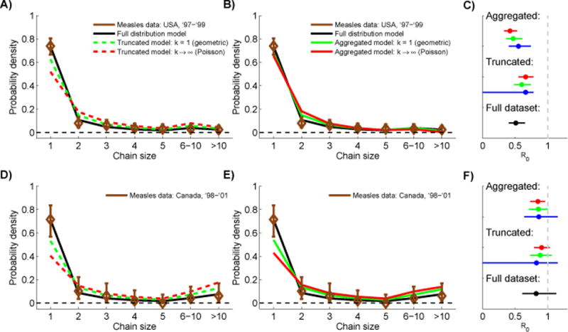
Plotting the measles data from the United States and Canada shows a noticeable upper tail to the chain size distributions that is suggestive of a high degree of transmission heterogeneity (figure 1A). The significance of this upper tail is highlighted when the data are plotted in terms of the distribution of chain size associated with a randomly chosen case (i.e. chain sizes are weighted in proportion to the number of cases they contain) (figure 1B). These observations highlight the importance of understanding how the number of isolated cases and the degree of transmission heterogeneity impact R₀ estimation.

Figure 1. Inference of R₀ and k for measles data.

A) Distribution of chain sizes for measles data in the United States (1997–1999) and Canada (1998–2001). B) Weighted distribution of the same data, showing the distribution of cases according to the size of the chain they belong to. C) Results of inferring R₀ and k for measles in the United States. Markers depict the maximum likelihood estimates (MLE) as determined by five different approaches. The full-distribution MLE assumes a negative binomial offspring distribution and uses the complete chain size distribution to infer both R₀ and k. The contour line shows the corresponding 95% confidence region. The truncated estimates only consider chains that are size two or greater. The aggregated estimates are based on the number of isolated cases, the total number of chains and the size of the largest chain. Both the truncated and aggregated estimates assume either a geometric offspring distribution with k = 1 (lower cross marks) or a Poisson offspring distribution with k → ∞ (higher cross marks). D) Analogous to panel C, but for measles in Canada.

Comparison of five previously published methods for estimating R₀ shows that each approach yields a distinct result when applied to measles data for the United States (figure 1C). Of the methods considered, the R̂_0,MLE estimate is the only one that incorporates all observed chain sizes. Further, while each method assumes that transmission by each case is independent of all other cases, the R̂_0,MLE method is the only one that makes no a priori assumptions about the degree of individual-level transmission heterogeneity. The ML estimate for R̂_0,MLE is 0.51 (95% CI: 0.40–0.65), which corroborates previous conclusions that local elimination has been sustained (i.e. there is no statistical support for R₀ > 1).

We consider two truncated methods, which ignore isolated cases and assume that the underlying offspring distribution is either geometric (R̂_0−T,k=1) or Poisson (R̂_{0−T,k→∞}) distributed. These methods estimate R₀ as 0.60 (95% CI: 0.48–0.74) and 0.66 (95% CI: 0.55–0.78) respectively, yielding estimates larger than R̂_0,MLE. This is because the R̂_0−T,k=1 and R̂_{0−T,k→∞} estimators assume a lower degree of transmission heterogeneity than is supported by the observed chain size distribution, and so they lead to higher R₀ estimates in order to fit the large chains in the observed truncated chain size distribution (discussed further in Appendix A.1 and Appendix B).

The two aggregated methods considered, R̂_0−A,k=1 and R̂_{0−A,k→∞}, do not distinguish different intermediate sized chains. These aggregated methods have the lowest R₀ estimates (R̂_0−A,k=1 = 0.47, 95% CI: 0.36–0.61; R̂_{0−A,k→∞} = 0.42, 95% CI: 0.33–0.53). This is because of the focus on isolated cases, which make up a relatively large fraction of the observed chains. Because these estimators assume relatively homogeneous transmission, which tends to give a low frequency of isolated cases, the estimated value of R₀ drops accordingly (discussed further in Appendix A.2 and Appendix B).

In analyzing the measles data from Canada, a few key differences are evident when the same five R₀ estimation methods are compared (figure 1D). Importantly, the R̂_0,MLE estimator shows that the data may be consistent with R₀ > 1 (R̂_0,MLE = 0.82, 95% CI: 0.61–1.13). The possibility of R₀ > 1 arises because the stochastic nature of transmission may cause all observed chains to stutter to extinction even though endemic transmission is feasible.

When the truncated estimators are applied to the Canadian measles data, their ML estimates again exceed R̂_0,MLE, for the same reasons as for the United States data (R̂_0−T,k=1 = 0.88, 95% CI: 0.73–1.06; R̂_{0−T,k→∞} = 0.91, 95% CI: 0.79–1.03). The truncated estimators also allow for the possibility that R₀ > 1, although their confidence intervals are narrower than for R̂_0,MLE because the probability of only observing self-limited clusters when R₀ > 1 is lower when transmission is assumed to be relatively homogeneous. In contrast to the analysis of United States data, when the aggregated estimators are applied to Canadian measles data they yield ML estimates exceeding R̂_0,MLE (R̂_0−A,k=1 = 0.85, 95% CI: 0.71–1.00; R̂_{0−A,k→∞} = 0.85, 95% CI: 0.73–0.96). This is because the very large Canadian chain containing 155 cases drives up R₀ estimates.

Previous analyses of measles in the United States (Gay et al., 2004) and Canada (King et al., 2004) used two R₀ estimation methods that are closely related to the methods we have considered above (to prevent crowding and keep the focus on the specific impact of truncated or aggregated chain size distributions, these estimates are not shown in figure 1C and 1D). One of these estimators equated R₀ with the fraction of non-imported cases. The corresponding R₀ estimates are 0.68 (95% CI: 0.60–0.78) for the United States data and 0.87 (95% CI: 0.76–0.98) for the Canada data. In principle this estimate should be identical to our R̂_0,MLE estimator (De Serres et al., 2000; Blumberg and Lloyd-Smith, 2013), but instead the earlier estimates are slightly higher because an imported case was not observed in all measles chains. The original analyses also conducted ML estimation of R₀ by assuming a Poisson offspring distribution and discarding both isolated cases and chains of size two. The resulting R₀ estimates are 0.63 (95% CI: 0.51–0.76) for the United States data and 0.87 (95% CI: 0.76–0.98) for the Canadian data.

3.2. Likelihood scores help to rule out some models

When chain size distribution models are compared to the original data and likelihood scores are calculated, the subtleties of the various estimation methods become more clear (figure B.8 and table 2). Focusing on the United States data, when all chain size data are used in the likelihood calculation (L_C), the best scores occur for the R̂_0,MLE prediction, as expected since this is the only method which uses the full chain size distribution. The only other model that is close is R̂_0−A,k=? (i.e. an aggregated estimator where k is inferred from the data). The data are clearly incompatible with homogeneous transmission, as seen by the fact that the two models that assume a Poisson offspring distribution have particularly low likelihoods. The truncated estimator models perform worse than the aggregated models, which is understandable since the number of isolated cases is included in the L_C calculation, but this information is not used in truncated estimation.

Figure B.8. Comparing model predictions to data.

A) Comparing United States measles data to predictions based on the complete chain size distribution (R̂_0,MLE) versus a truncated distribution (R̂_0−T,k=1 and R̂_{0−T,k→∞}). Errors bars show 95% confidence intervals for proportions of each chain size in the data. Table 2 contains the likelihood scores for each set of predictions. B) Similar to panel A but the R̂_0,MLE model is now compared to predictions based on aggregating intermediate chain sizes (R̂_0−A,k=1 and R̂_{0−A,k→∞}). C) ML values of R₀ for the models shown in panels A and B along with the 95% confidence intervals. Green confidence intervals correspond to a geometric distribution, red confidence intervals are for a Poisson offspring distribution and blue confidence intervals are for when k is inferred. (The numeric values for the confidence intervals are all provided in section 3.1.) D–F) Analogous to panels A, B and C, except that estimator predictions are compared to data for measles in Canada. For the R̂_0,MLE, R̂_0−T,K=? and R̂_0−A,K=? estimators, the associated k̂ values are 0.32, ∞ and 0.27 for measles in the United States. The corresponding k̂ values are 0.21, 0.23 and 0.20 for measles in Canada.

Table 2. Log likelihood scores for measles data from the United States and Canada.

The relative log likelihood scores are either based on all observed chains (ΔL_C) or on the truncated distribution in which isolated cases are discarded (ΔL_T). The R̂_0,MLE calculation is used as the reference point for both ΔL_C and ΔL_T. Positive values of ΔL_C and ΔL_T correspond to higher likelihood values than the reference.

	USA Measles (’97–’99)		Canada Measles (’98–’01)
Estimator	ΔLC	ΔLT	ΔLC	ΔLT
R̂0,MLE	0.0	0.0	0.0	0.0
R̂0−T,k=1	−4.5	0.3	−3.6	−0.1
R̂0−T,k→∞	−16.3	0.6	−10.1	−0.5
R̂0−T,k=?	−16.3	0.6	0.0	0.0
R̂0−A,k=1	−3.3	−1.8	−3.4	−0.2
R̂0−A,k→∞	−12.9	−10.2	−9.1	−1.0
R̂0−A,k=?	−0.3	−0.3	−0.1	−0.1

When isolated cases are removed from the likelihood calculation, differences among the resulting likelihood scores (L_T) are smaller. The smaller differences arise in part because fewer data points are used and in part because the most significant model discrepancies for L_C concern the predicted number of isolated cases. Interestingly, while the assumption of a Poisson offspring distribution provides the highest L_T for the truncated estimators for the United States data, this assumption provides the lowest likelihood for the aggregated estimators. This highlights the potential for inconsistency between estimation of R₀ based on truncated versus aggregated chain size distributions.

Since all chain size data are used for inference, a completely independent set of data is not available to test the model predictions. However, data on the number of generations of transmission before extinction can also be used for inference of R₀ (Gay et al., 2004; Farrington et al., 2003) and the likelihood of these data can be used as an additional basis for model comparison. For United States data (Gay et al., 2004), model comparison results based on generation of extinction parallel those based on chain size distributions, with the R̂_0,MLE and R̂_0−A,k=? estimators having the highest likelihoods (Appendix C). This consistency across model comparisons is re-assuring and supports the use of branching process theory to describe transmission.

The likelihood scores obtained when the different estimators are applied to the Canadian measles data show similar trends to the United States analyses (table 2). The main difference is that the magnitudes of the likelihood differences are smaller, in large part because the data set is smaller.

3.3. Evaluating the potential bias caused by imperfect observation of cases

The truncated and aggregated estimators were designed to address the reality of imperfect case observation (De Serres et al., 2000; Ferguson et al., 2004; Farrington et al., 2003). However a head-to-head comparison of these estimators in the context of different assumptions about the observation process has not been performed. For instance, the truncated estimators are based on the reasonable conjecture that the number of isolated cases would be the least accurate component of the chain size distribution (De Serres et al., 2000). However, any observation errors that affect the isolated case count may also decrease the observed size of larger stuttering chains. In this case, it is less clear that the truncated estimators would perform better than an estimator that is based on all observed chain sizes. To understand how different estimation approaches are impacted by imperfect observation, we determined the estimation bias when R₀ inference is performed on simulated data subject to independent or size-dependent observation.

3.3.1. Independent observation error decreases R₀ estimates

In the independent observation model, many small chains will be completely unobserved and large chains are likely to appear smaller than they actually are. Thus the observed number of smaller chains will represent a mix of some chains that are truly the specified size and some larger chains that are only partially observed.

When we simulate imperfect data using the independent observation model, the resulting bias in R₀ estimation depends on the transmission parameters, the observation probability and the estimator utilized (figure 2). In general, the bias becomes more negative as observation probability declines. In the case of the full-distribution and truncated estimators, this is because the observed average chain size decreases as observation probability decreases (figure A.5A). For the aggregated estimators, it is because independent observation error potentially increases the observed number of isolated cases, while likely decreasing the observed size of the largest chain. In many circumstances, it appears that the fraction of cases unobserved would have to be substantial (i.e. around 50%) in order for there to be a significant change in bias (i.e. a decrease of 0.1) relative to perfect observation. This blunted dependence of bias on observation probability is due to the average chain size growing faster than linearly with R₀. For the full-distribution and truncated estimators, excellent agreement between analytical (equations 16 and 17) and simulation results confirms that the estimator bias is primarily a function of the observed average chain size (data not shown).

Figure 2. Absolute bias of R₀ estimation associated with independent observation error.

Simulated observation scenarios used to measure absolute bias are created by assuming that each case has an independent and identical probability of being detected. The curves in each panel show how the bias varies as a function of the observation probability and estimator choice. Results are shown for the R̂_0,MLE, R̂_0−T,k=1, R̂_{0−T,k→∞}, R̂_0−A,k=1 and R̂_{0−A,k→∞} estimators. Each panel corresponds to a different pair of true R₀ and k values.

Figure A.5. Evaluating R₀ estimators when data sets are truncated by ignoring isolated cases.

A) Size of stuttering chains as a function of R₀. The average size of all chains, μ, is independent of k (black line, equation 2). Meanwhile, the average size of chains containing at least one secondary infection, μ_s, depends on k (colored lines, equation 8 with p_obs = 1). B) Root mean square absolute error of the R₀ estimate (equation 14) as a function of the true dispersion parameter. The R̂_0,MLE estimator (which uses the full chain size distribution) is shown for reference. As explained in the text, the truncated estimators differ only in the way they model transmission heterogeneity. The colored lines correspond to R̂_0−T,k=? (blue) R̂_0−T,k=1 (green), R̂_{0−T,k→∞} (red), and R̂_{0−T,k=k^′} (magenta) and are all based on equation 11. The true R₀ is fixed at 0.5. The qualitative behavior is similar for different values of R₀ (data not shown). C) Fraction of the absolute error shown in panel B that is due to estimation bias (equation 18). D) Coverage probability of the 95% confidence intervals for the same estimators and transmission parameters shown in panel B. In panels B–D, each data point is based on 2000 simulations. To minimize the effects of sampling variance, N = 1000 for all simulations. The full-distribution (R̂_0,MLE) results are hidden in panels B–D because they are essentially identical to the performance of R̂_{0−T,k=k^′}.

Paradoxically, when estimating R₀ there may be circumstances in which two wrongs make a right, as the bias due to imperfect observation can balance out the bias due to incorrect assumptions about transmission heterogeneity. For instance, assuming a higher k than the true value can compensate for the bias of truncated estimators under independent observation error (seen when dashed lines cross the x-axis in figures 2A and 2B). These paradoxical circumstances should be distinguished from those circumstances in which bias is minimized because the assumptions of the inference methods accurately reflect the mechanisms of transmission and case observation.

3.3.2. Size-dependent observation, which increases R₀ estimates, can sometimes be compensated for by truncated estimation methods

In the size-dependent observation model, large chains are likely to be observed in their entirety but small chains and isolated cases are likely to be under-counted. Thus when the observation process follows the size-dependent model, the bias becomes more positive as the overall observation probability decreases (figure 3).

Figure 3. Absolute bias of R₀ estimation associated with size-dependent observation error.

The panels are analogous to those in figure 2 except that each case has an identical and independent probability of being a sentinel case that activates complete observation of the chain they are part of. Chains without a sentinel case are not observed at all. The observation probability plotted here is the overall probability that a randomly chosen case is observed, which can be significantly higher than the probability of being a sentinel case (equation 6).

Importantly, with size-dependent observation, the truncated estimators are consistently less biased than R̂_0,MLE when the assumed transmission heterogeneity matches the true heterogeneity (best seen by comparing the black and dashed red lines in figures 3C and 3D). Of course, this reflects the original intention that truncated estimators would apply to data for which accurate reporting of large chains is favored over reporting of small chains. However this benefit can be dramatically reversed when the estimator underestimates the true degree of transmission heterogeneity (figure 3A). Thus excluding isolated cases from data analysis is reasonable if there is convincing evidence that isolated cases are more prone to surveillance bias than cases in large chains, but accurate assumptions about heterogeneity remain important. In circumstances where case detection is perfect, truncating data runs the risk of introducing bias or expanding the confidence intervals more than necessary (figure A.5).

The aggregated estimators are the most sensitive to size-dependent observation (best seen in the solid colored lines of figures 3B and 3C). This is consistent with the aggregated estimators’ focus on the observed number of isolated cases, because size-dependent observation is particularly prone to missing these cases.

3.4. Correcting for imperfect observation is feasible when the observation process is well-characterized

Until now we have acknowledged that surveillance data suffer from observation error, but have always inferred R₀ with the assumption that the data are good enough to be taken at face value. Following earlier work, the hope was that a work-around solution (i.e. truncated or aggregated estimation) may avoid the need to correct explicitly for imperfect observation. However, if the mechanisms underlying imperfect observation correspond well to a simple model and the overall observation probability can be quantified, then it is straightforward to adjust R̂_0,MLE accordingly so that inference remains unbiased.

To explore this possibility, we re-analyzed the measles data sets subject to the assumption that the observation model and observation probability were known. Correcting for independent observation probability increased the R₀ estimates for measles, and correcting for size-dependent observation decreased the estimates (figure 4 and table 3). However the differences in likelihood scores are very small. This suggests there is little information content from which to infer observation probabilities from these chain size distributions. Instead, the natural tradeoff between observation probability and R₀ estimates implies additional data are needed to choose an appropriate observation model and infer observation probabilities.

Figure 4. Inference of R₀ when imperfect observation is incorporated into the likelihood calculation.

A) The 95% contour and ML value for R₀ and k for measles in the USA is shown for three different assumptions about the observation process. The black contour assumes all cases are observed. The green contour assumes each case is observed with an independent probability of 50%. The blue contour assumes each case has a 50% probability of being a sentinel case that activates complete observation of the chain it is part of. B) Analogous to panel A but for measles in Canada.

Table 3. Log likelihood scores based on different observation models for measles data.

The ‘perfect observation’ model, corresponding to R̂_0,MLE, is used as the likelihood reference point. The ML values for R₀ and associated 95% confidence intervals are also shown

Observation model	USA Measles (’97–’99)		Canada Measles (’98–’01)
	ΔLC	R̂0	ΔLC	R̂0
Perfect observation	0.0	0.51 (0.40 – 0.65)	0.0	0.82 (0.61 – 1.13)
50% independent observation	0.1	0.59 (0.48 – 0.71)	−0.1	0.85 (0.66 – 1.10)
50% sentinel case probability	0.6	0.38 (0.28 – 0.51)	−0.5	0.73 (0.49 – 1.12)

Unexpectedly, the confidence intervals tend to shrink rather than expand when observation is imperfect. This is due to the peculiarity that when the observation probability is low, many more chains occur than are actually observed. As an extreme example, it becomes less likely that R₀ > 1 and only finite sized chains are observed when the observation probability is low, because it is likely that at least one primary case (even if it was not observed) would lead to a chain that escapes extinction. Another intriguing outcome of this exploration is that correcting for imperfect observation tends to decrease the maximum likelihood value of k (figure 4). This suggests that whenever the R̂_0,MLE infers a high degree of heterogeneity under the assumption of perfect observation, the true degree of heterogeneity might be even greater.

4. Discussion

Given the potential global impact of emerging and re-emerging infectious diseases, it is not surprising that a number of techniques have been developed to analyze the stuttering chains that are the hallmark of subcritical transmission. Our goal has been to quantitatively compare these techniques, amidst a variety of assumptions about transmission heterogeneity and case observation. Our use of a negative binomial offspring distribution to model the complete chain size distribution provided a unified foundation for our study, because it allowed a flexible degree of transmission heterogeneity and could be easily modified to accommodate different observation models.

Imperfect observation is a reality of collecting data on sporadic stuttering transmission chains, and so there is a compelling need to understand how this challenge impacts various approaches to R₀ estimation. This has been a major focus of this manuscript, but in order to develop a theoretical framework for understanding the impact of imperfect observation, we first examined how different estimators perform on perfect data. When inference is based on the complete or aggregated chain size distribution, we found that treating k as a free parameter leads to the smallest estimation errors and most reliable confidence intervals (Appendix A). This contrasts with the standard practice of assuming either a geometric or Poisson offspring distribution. However, it is difficult to assess the degree of transmission heterogeneity from a truncated distribution (Appendix A.1). This is a problem because improper assumptions concerning the degree of heterogeneity can introduce bias in truncated estimation of R₀ and lead to unreliable confidence interval coverage (figure A.5).

The potential dangers of using a truncated estimator are highlighted in our analysis of measles. It seems more likely that isolated measles cases would be under-observed than over-observed, because isolated cases require astute clinical intervention in order to activate national surveillance protocols. However, the best-fit predictions of the truncated estimators all underestimate the observed number of isolated cases (figures B.8A and B.8D). An alternative explanation for the high observed proportion of isolated cases is that there is a high degree of transmission heterogeneity. When k is allowed to be a free parameter in the R̂_0,MLE or R̂_0−A,k=? estimators, the number of isolated cases is predicted accurately (figures B.8B and B.8E). Ironically, specific assumptions concerning the degree of transmission heterogeneity can lead to inconsistency between the motivation for truncating isolated cases (which can be beneficial for size-dependent observation) and the use of truncated estimators. In particular, our explicit correction for size-dependent observation led to a decreased estimate for R₀ relative to R̂_0,MLE (figure 4 and table 3) while use of R̂_{0−T,k→∞} produced a higher estimate than R̂_0,MLE (figures 1C and 1D). The crux of this inconsistency is our finding that poorly modeled heterogeneity can sometimes overwhelm the bias due to imperfect observation (figures 2 and 3).

The strong performance of aggregated estimators for perfectly observed data suggests that there may be circumstances where resources should be deployed to optimize accurate counts of isolated cases, total chains and the size of the largest chains, without spending extra effort characterizing intermediate-sized chains. We note, however, that these circumstances will be difficult to identify a priori, and that this surveillance design would sacrifice other benefits accruing from fully characterizing all transmission chains. Also, when data are sparse the use of an aggregated distribution can lead to larger confidence intervals for R₀ estimation than when the full chain size distribution is used.

The challenge of imperfect observation is complicated by the many reasons that cases can go unobserved. Cases may be missed due to laboratory errors, logistical hurdles of acquiring samples in a timely manner, failure to report suspected cases, or subclinical infections that do not garner medical attention. Since each of these mechanisms can have a distinct impact on the observed chain size distribution (e.g. subclinical infections may affect each case independently, while delayed recognition of outbreaks may cause large chains to have higher observation probabilities), different observation process models are applicable in different scenarios. Our consideration of independent observation and size-dependent observation provides an initial characterization of how imperfect observation impacts inference of R₀. However our treatment is far from complete as other types of observation error may be present. For instance, it is sometimes difficult to differentiate one transmission chain from another, and improper assignment of cases to chains can affect the recorded chain size distribution.

Overall, our simulation studies and analysis of measles data emphasize the need for inference approaches that address imperfect observation based on mechanistic adjustments to the likelihood function. When reliable information exists concerning the mechanism of imperfect observation and the overall observation probability, then the likelihood calculation can incorporate imperfect observation explicitly (figure 4). Major challenges in correcting for imperfect observation are that the overall observation probability is often unknown and it is unclear which observation model is most suitable. As we found with our analysis of measles, this type of information is difficult to obtain solely from the chain size distribution (table 3), suggesting the importance of gathering additional data with which to study these essential processes.

5. Conclusions

Analysis of measles data showed that existing methods for inference of R₀ from chain size data yield distinct results (figure 1). To reconcile these differences we used simulation studies to show that improperly modeled heterogeneity leads to bias in R₀ estimation. This bias can be positive or negative depending on which part of the chain size distribution is used for inference and how heterogeneity is modeled. When observation is perfect, we found that allowing a flexible degree of heterogeneity led to the smallest bias.

Meanwhile, the reality of imperfect observation cannot be avoided, and prior approaches to estimating R₀ with a truncated or aggregated chain size distribution were designed with this limitation in mind. Unfortunately, truncated estimators are often problematic because ignoring isolated cases makes it difficult to infer the degree of heterogeneity, which can produce large estimation errors even when observation is perfect. Meanwhile, aggregated estimators can be very sensitive to error in the observed number of isolated cases.

As a way forward, we have shown that the observation process can be incorporated directly into the likelihood of the observed chain size distribution. This provides a unified approach for incorporating a flexible degree of heterogeneity and a mechanistic observation model into inference of R₀. This offers the potential to make unbiased inference from imperfect data.

A key shortcoming is that many empirical reports do not include quantitative descriptions of the observation process. This makes it difficult to determine the overall observation probability and what mechanisms govern observation error. We hope that our results will stimulate new surveillance strategies that allow more explicit characterization of the observation process. For instance, future studies may find that knowing the number of cases that were retrospectively identified, or the fraction of chains containing a known primary infection is helpful for estimating the overall observation probability. This type of integrative approach will improve our ability to reliably monitor emerging diseases that are a risk for endemic or epidemic spread.

Highlights.

1. Previous analyses of subcritical disease transmission have used several approaches to estimate R₀ from chain size distributions.

2. Imperfect observation and assuming a specific amount of transmission heterogeneity can both bias estimation of R₀.

3. The estimation bias can be corrected by incorporating the observation process and a flexible degree of transmission heterogeneity into models of chain size distributions.

Appendix A. Comparing R̂_0,MLE to other R₀ estimation methods

Having observed significant differences when applying the various R₀ estimators to epidemiological data (figure 1), we conducted a set of simulation studies in order to understand the nature of the discrepancies. In particular, we explored how different degrees of transmission heterogeneity affect the estimation of R₀ from perfectly observed simulated data using truncated and aggregated estimators.

Appendix A.1. Accurate and precise estimation of R₀ from truncated data requires that the degree of heterogeneity be known accurately a priori

The expected mean chain size in truncated data sets, μ_s, depends on the degree of transmission heterogeneity (figure A.5A). For fixed μ_s, the estimated R₀ increases as the assumed value of k increases. Therefore, the higher the assumed or inferred value of k, the higher the estimate of R₀ from truncated data will be.

When the number of data points is large, the error of estimating R₀ from a truncated distribution for which the true k is known (R̂_{0−T,k=k^′}) is similar to the error of estimating R₀ from the full chain size distribution (R̂_0,MLE) (figure A.5B). However the error is relatively large when a truncated distribution is used and k is inferred (R̂_0−T,k=?). Meanwhile, when a geometric or Poisson offspring distribution is assumed (R̂_0−T,k=1 or R̂_{0−T,k→∞}), the error of the truncated estimator error is negligible only when the true value of k is close to its assumed value (i.e. when k is close to 1 or approaches ∞ respectively).

Examination of the fraction of error due to bias (ρ) shows that when a specific value for k is chosen, up to ninety percent of the error in estimating R₀ from a truncated distribution is due to bias when the true k is far from the assumed value (Fig A.5C). In contrast, the fraction of error is essentially zero when the true value of k matches the assumed value. Because μ_s decreases as k increases, k = 1 marks the point for which the bias of R̂_0−T,k=1 goes from positive to negative. Meanwhile, the bias of R̂_{0−T,k→∞} is always positive. Interestingly, despite the relatively large error of estimating R₀ when k is inferred from a truncated distribution, the fraction of this error due to bias is relatively small. Taken together these results indicate that when isolated cases are ignored, knowledge of k is important for precise and unbiased R₀ inference. However, based on the imprecision of the R̂_0−T,k=? estimator, it appears difficult to precisely determine k from a truncated chain size distribution.

When a value of k is assumed, the 95% coverage probability of the truncated estimators shows that the calculated confidence intervals are only accurate when the true k is close to the assumed value (Fig A.5D). In contrast, when k is inferred from the truncated distribution, the coverage probability tends to exceed 95% suggesting that the confidence intervals are too permissive. These coverage probability results indicate a tradeoff when using a truncated likelihood for whether or not to fix k. The benefit of fixing a value for k is a more precise estimate that works well if k is fairly accurately known. However if the degree of transmission heterogeneity is unknown, then assigning a specific value for k brings the risk of a biased estimate with falsely narrow confidence intervals, resulting in an over-estimation of accuracy. In contrast, inferring R₀ from truncated chain size distributions while allowing a flexible value for k has the potential advantage of conservative confidence intervals, but the disadvantage of larger uncertainties.

Appendix A.2. Accurate and precise estimation of R₀ from aggregated data does not require a priori knowledge about transmission heterogeneity

When intermediate-valued chain sizes are aggregated together, the likelihood function is strongly influenced by the size of the largest observed chain, which in turn depends on R₀, k and N (figure A.6A). The largest chain is sensitive to R₀ and k because these parameters impact the expected chain size distribution, but there is also a dependence on the size of the data set because the explosive potential of heterogeneous transmission may only be evident when there are many stuttering chains in a data set. These features provide the intuitive foundation for understanding why improper assumptions about k can lead to biased R₀ estimates when the likelihood is based on an aggregated chain size distribution.

Figure A.6. Evaluating R₀ estimators in which intermediate stuttering chain sizes are aggregated together.

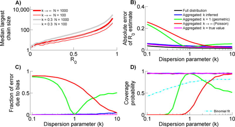
A) Across many simulated chain size distributions, the median size of the largest chain depends on R₀, k and the number of observed chains, N. B–D) Analogous to panels B–D in figure A.5 except that the colored curves correspond to the aggregated estimators based on equation 12: R̂_0−A,k=? (blue) R̂_0−A,k=1 (green), R̂_{0−A,k→∞} (red), and R̂_{0−A,k=k^′} (magenta). The full-distribution results are hidden in panels C and D, because they are essentially identical to the aggregated results when k is either known or inferred. The binomial estimator, R̂_0,binomial, which has the same value but different confidence intervals than the full-distribution estimator, is based solely on the fraction of cases that are secondary (equation 13, cyan line in panel D).

When the true k is used, R₀ estimation based on an aggregated chain size distribution is unbiased, the absolute error is essentially as good as or better than all other estimators, and the 95% coverage probability is appropriately valued (Figures A.6B–D). When a particular value of k is assumed (e.g. R̂_0−A,k=1 and R̂_{0−A,k→∞}), one sees qualitatively similar trends as the corresponding truncated likelihood functions (e.g. R̂_0−T,k=1 and R̂_{0−T,k→∞}). Namely, when the true k differs from the assumed k, the absolute error increases due to worsening bias. Interestingly, when no assumptions are made about k and it is inferred from the data, the absolute error of aggregated estimation (e.g. R̂_0−A,k=?) is remarkably close to that obtained from using the full chain size distribution. Further, R̂_0−A,k=? is unbiased and the 95% coverage probability is appropriately valued. This is consistent with prior observations that the fraction of chains that are isolated cases provides useful information for inference of k from contact tracing data (Lloyd-Smith et al., 2005; Lloyd-Smith, 2007). Overall, this supports the assertion that the key content of the stuttering chain size distribution can be summarized by relatively few parameters (Ferguson et al., 2004), but argues against predetermining the appropriate value of k when using an aggregated likelihood. Nevertheless, it is still preferable to use R̂_0,MLE when complete chain size data are available, because for small datasets the absolute error and the associated confidence interval of R̂_0−A,k=? can be twice as large as the values based on complete distribution (data not shown).

The observation that R̂_0−A,k=? performs comparably to R̂_0,MLE motivates the possibility that an even simpler likelihood function can be derived that depends only on the fraction of cases that are secondary infections. Since the corresponding ML estimate, R̂_0,binomial, is identical to R̂_0,MLE, the absolute bias and error of these two estimators are identical. However, the same is not true for the coverage probability. Rather, the L_B function over-estimates the accuracy of R̂_0,binomial, particularly when transmission heterogeneity is significant (figure A.6D). This result shows that while an unbiased R₀ estimate can be obtained from knowing just the fraction of cases due to secondary transmission, accurate confidence intervals require more information about the distribution of chain sizes.

Appendix A.3. Simulations based on a Weibull-Poisson offspring distribution confirm results based on a negative binomial offspring distribution

The results of section A.1 and A.2 are potentially circular as the simulations and inference methods all assume a negative binomial offspring distribution. To check whether the results are robust to an alternate choice of offspring distribution, we performed identical analysis (e.g. inference remains based on a negative binomial offspring distribution) on simulations using a Weibull-Poisson offspring distribution (figure A.7).

Figure A.7. Comparing R₀ estimators when simulations are based on a Weibull-Poisson offspring distribution.

A–C) Analogous to figure A.5B–D but based on a ‘matched’ Weibull-Poisson distribution. D–F) Analogous to figure A.6B–D.

To compare results for simulations based on Weibull-Poisson offspring distribution to those based on a negative binomial offspring distribution, we had to identify a mapping between the two parameters that describe the distributions. The negative binomial distribution is equivalent to a Gamma-Poisson mixture. Mathematically, this is equivalent to choosing an individual reproductive number based on a Gamma distribution and then determining the number of offspring according to a Poisson distribution with a mean equal to the chosen reproductive number (Lloyd-Smith et al., 2005). Thus one can think of a negative binomial offspring distribution as corresponding to a gamma-distributed infectious period and a Weibull-Poisson offspring as corresponding to a Weibull-distributed infectious period (assuming transmission is constant during the infectious period). For a given, R₀ and k, the ‘matched’ Weibull-Poisson distribution was determined by first identifying the matched Weibull distribution that had a mean and variance equal to that of a Gamma distribution with parameters R₀ and k. Then, the equivalent Weibull-Poisson distribution was found by simulating many draws from a Poisson distribution with a mean chosen from the matched Weibull distribution.

Overall, the new set of results confirms the trends seen in figures A.5 and A.6, but there are a few subtle differences. For one, the aggregated estimator, R̂_0−A,k=?, no longer performs as well as R̂_0,MLE. In addition, the error of R̂_0,MLE is slightly higher and its coverage probability drops for low k. This is understandable because R̂_0,MLE no longer represents a model that is an exact match of the simulation model. Overall though, the performance of R̂_0,MLE is still very robust and for many purposes the performance of R̂_0−A,k=? may also be adequate. In contrast to our initial set of simulations, the R̂_{0−A,k=k^′} performs worse than R̂_0−A,k=? when k is small, presumably because the negative binomial and Weibull-Poisson distributions have quite different shapes in this limit.

Appendix B. Comparison of data to model predictions

As is evident in the analysis of the United States measles data, models based on the truncated estimators (R̂_0−T,k=1 and R̂_{0−T,k→∞}) predict significantly fewer isolated cases than were actually observed (figure B.8A). The discrepancy is greater for the R̂_{0−T,k→∞} model than for the R̂_0−T,k=1 model. Since heterogeneous transmission causes more variance in the stuttering chain size distribution, this suggests that the truncated data would be better modeled by allowing more transmission heterogeneity in the offspring distribution. This conclusion is supported by the ML estimate of 0.3 (95% CI: 0.2 – 0.8) for k when the likelihood is based on the full chain size distribution. An alternative explanation for this discrepancy between data and the truncated estimator predictions is that there is a preponderance of false positive isolated cases. However, for the best agreement with the data, 15% and 30% of the observed isolated cases would have to be false-positive infections for the R̂_0−T,k=1 and R̂_{0−T,k→∞} predictions respectively. These proportions seem implausibly high, and would need to be even higher if true isolated cases are also more prone to be missed by surveillance.

The aggregated estimator model predictions show good agreement with the number of isolated cases for measles in the United States, but poorer agreement with the number of chains of size two (figure B.8B). This is consistent with the aggregated likelihood calculation’s explicit emphasis on the number of isolated cases and lack of emphasis on the specific distribution of intermediate sized chains. The mismatch of size two chains is worse for R̂_{0−A,k→∞} than for R̂_0−A,k=1, which is consistent with the ML value of 0.27 for k obtained using the R̂_0−A,k=? method.

The model predictions illustrate that relative to the data for measles in the United States, the truncated models shift more of the probability distribution to higher chain sizes (i.e. lower probability for isolated cases) while the aggregated models shift more of the probability distribution to smaller chain sizes (i.e. a higher probability for isolated cases must be balanced by lower probabilities for large chains). This explains why the truncated estimators tend to have higher values than R̂_0,MLE, while the aggregated estimators have lower values (figures 1C and B.8C). Meanwhile, when all truncated and aggregated models are compared together, the narrowest confidence intervals occur when a Poisson offspring distribution is assumed and the widest confidence intervals occur when k is inferred. This is because the assumption of homogeneous transmission implies that there is less statistical variance in the data. However, because inaccurately modeled heterogeneity can introduce bias, this does not necessarily mean that the Poisson-based confidence intervals are more accurate (figures A.5D and A.6D). Meanwhile, when k is allowed to vary, the confidence intervals incorporate the possibility of low k which implies the potential for large statistical variance and thus wider confidence intervals.

Analysis of measles data for Canada shows the same trend of the truncated estimator models predicting fewer isolated cases than are found in the data (figure B.8D). However, the Canadian models differ from the United States models in that a higher fraction of large chains are predicted. This is largely driven by the existence of a chain of size 155 in the Canadian data. This large chain also causes a heavier upper tail in the aggregated model predictions (figure B.8E). In fact the aggregated models’ focus on the size of the largest cluster combined with constraints of assuming a Poisson or geometric offspring distribution cause a natural tension between fitting the number of isolated cases and the upper tail of the distribution. Because of the large chain, the aggregated models do a poorer job at fitting the number of isolated cases and thus there is not much difference with the truncated model predictions. The similarities between the aggregated and truncated predictions lead to similar ML values for R₀ and associated confidence intervals (figures 1D and B.8F). As with the United States analysis, the Canadian confidence intervals show a similar trend of having particularly wide intervals when k is inferred. Overall, the Canadian confidence intervals are wider because there are fewer chains in the data set.

Appendix C. Model predictions for the generation of extinction

Past work has shown that the distribution for the generation in which chains go extinct is dependent on R₀ (Farrington et al., 2003). While generation of extinction data is not entirely independent of chain size data, analyzing the generation of extinction data helps to confirm the results of Appendix B and provides an overall validation of using branching process theory to describe disease transmission. Here we review the theory for determining the distribution for the generation of extinction. Then we compare predictions for USA and Canada measles.

Appendix C1. Theory for the generation of extinction

The generating function for a negative binomial offspring distribution is,

$$Q(s)={(1+\frac{R_0}{k}(1-s))}^{-k}$$

We define the primary case of a chain to be the first generation of a chain. The probability that a chain goes extinct after one generation (i.e. that the primary case is a dead-end for transmission), q1, is Q(0) (Harris, 2002; Lange, 2010). The probability that a generation goes extinct after z generations, q_z, is Q(q_z−1). Thus the probability distribution for the generation of extinction can be determined recursively. This dependence can be used to infer R₀ (Gay et al., 2004), but we do not consider this type of inference in our current study.

If data exist on the generation of extinction, and there are u_z number of chains that have a generation of extinction of z, then the overall likelihood for the complete generation of extinction distribution is,

$$L_C^G={\displaystyle \prod }_{z=1}^{\infty }{q}_z^{u_z}$$ (C.1)

By analogy to the truncated likelihood for chain size distributions, a truncated generation of extinction likelihood can also be calculated by ignoring isolated cases. Since the first generation of a chain always has exactly one case, this is equivalent to only including chains in which the generation of extinction is at least two. Thus,

$$L_T^G={\displaystyle \prod }_{z=2}^{\infty }{\left(\frac{q_z}{1-q_1}\right)}^{u_z}.$$ (C.2)

Appendix C.2. Generation of extinction data

The generation of extinction was recorded for the United States measles data (see table 2 in Gay et al.), but could not be found for measles in Canada. There are a couple chains that were noted to have no spread, but also included more than two cases. Since the make-up of these chains were unclear, we chose to include these chains with the 122 isolated cases that go extinct in the first generation.

Appendix C.3. Model predictions for the generation of extinction

Based on estimated R₀ and either assumed or estimated k values, the distribution for the generation of extinction can be predicted (figure C.9). In general, the estimators that predict higher values for R₀ also predict a higher number of chains with long durations. Consistent with chain size analysis for measles in the United States, the truncated estimators predict fewer chains having an extinction generation of one (i.e. isolated cases) than the full-distribution and aggregated estimators. The general agreement between model predictions and data for measles in the United States confirms that branching processes are a reasonable model for subcritical transmission of measles.

Figure C.9. Model predictions for the generation of extinction.

A) Predictions for the generation of extinction for measles in the United States. The predictions are based on the inferred value of R₀ and either the assumed or inferred value of k for some of the estimators presented in the main text. The reported data are also shown along with 95% confidence intervals for the proportion of chains that went extinct in each generation. B) Analogous to panel A but for measles in Canada. Unfortunately, data are not available for comparison to model predictions.

Since the generation of extinction are available for measles in the United States, the likelihoods of these data can be compared (table C.4). In general the relative likelihoods based on the generation of extinction parallel those for chain size distributions (table 2). In particular, when all chains are included in the calculation $(L_C^G)$, scores are best when a significant degree of heterogeneity is allowed, and the aggregated estimators perform better than the truncated estimators. In contrast to our chain size analysis, the likelihood based on the generation of extinction for the R̂_0−A,k=? estimator exceeds that of R̂_0,MLE, but the difference is not statistically significant. When the likelihood is based on the truncated generation of extinction distribution $(L_T^G)$, the three models based on the truncated estimators perform best. The discrepancy between the best performance for $L_C^G$ and $L_T^G$ once again highlights the significance of isolated cases.

Table C.4. Log likelihood scores for generation of extinction data for measles in the United States.

The relative log likelihood scores are either based on all observed chains $(\mathrm{\Delta }{L}_C^G)$ or on the truncated distribution in which isolated cases are discarded $(\mathrm{\Delta }{L}_T^G)$. The R̂_0,MLE calculation is used as the reference point for both likelihood calculations. Positive values of $\mathrm{\Delta }{L}_C^G$ and $\mathrm{\Delta }{L}_T^G$ correspond to higher likelihood values than the reference.

	USA Measles (’97–’99)
Estimator	$\mathrm{\Delta }{L}_C^G$	$\mathrm{\Delta }{L}_T^G$
R̂0,MLE	0.0	0.0
R̂0−T,k=1	−3.6	2.2
R̂0−T,k→∞	−16.7	2.1
R̂0−T,k=?	−16.7	2.1
R̂0−A,k=1	−2.5	−0.5
R̂0−A,k→∞	−5.8	−2.3
R̂0−A,k=?	1.0	1.0

References

- Antia R, Regoes RR, Koella JC, Bergstrom CT. The role of evolution in the emergence of infectious diseases. Nature. 2003;426:8–11. doi: 10.1038/nature02104. [DOI] [PMC free article] [PubMed] [Google Scholar]
- Arinaminpathy N, McLean AR. Evolution and emergence of novel human infections. Proceedings of the Royal Society B: Biological Sciences. 2009;276:3937–43. doi: 10.1098/rspb.2009.1059. [DOI] [PMC free article] [PubMed] [Google Scholar]
- Ball FG, Britton T, O’Neill PD. Empty confidence sets for epidemics, branching processes and brownian motion. Biometrika. 2002;89:211–224. [Google Scholar]
- Bauch CT, Earn DJD. Vaccination and the theory of games. Proceedings of the National Academy of Sciences of the United States of America. 2004;101:13391–4. doi: 10.1073/pnas.0403823101. [DOI] [PMC free article] [PubMed] [Google Scholar]
- Becker N. On parametric estimation for mortal branching processes. Biometrika. 1974;61:393–399. http://biomet.oxfordjournals.org/content/61/2/393.full.pdf+html. [Google Scholar]
- Becker N. Estimation for discrete time branching processes with application to epidemics. Biometrics. 1977;33:515–522. [PubMed] [Google Scholar]
- Blumberg S, Lloyd-Smith JO. Inference of R0 and transmission heterogeneity from the size distribution of stuttering chains. PLoS Computational Biology. 2013;9:e1002993. doi: 10.1371/journal.pcbi.1002993. [DOI] [PMC free article] [PubMed] [Google Scholar]
- Bolker BM. Ecological Models and Data in R. Princeton University Press; 2008. [Google Scholar]
- De Serres G, Gay NJ, Farrington CP. Epidemiology of transmissible diseases after elimination. The American Journal of Epidemiology. 2000;151:1039–1048. doi: 10.1093/oxfordjournals.aje.a010145. [DOI] [PubMed] [Google Scholar]
- Dwass M. The total progeny in a branching process and a related random walk. Journal of Applied Probability. 1969;6:682–686. [Google Scholar]
- Farrington CP, Kanaan MN, Gay NJ. Branching process models for surveillance of infectious diseases controlled by mass vaccination. Biostatistics. 2003;4:279–95. doi: 10.1093/biostatistics/4.2.279. [DOI] [PubMed] [Google Scholar]
- Ferguson NM, Fraser C, Donnelly CA, Ghani AC, Anderson RM. Public health risk from the avian H5N1 influenza epidemic. Science. 2004;304:1–5. doi: 10.1126/science.1096898. [DOI] [PubMed] [Google Scholar]
- Garske T, Rhodes CJ. The effect of superspreading on epidemic outbreak size distributions. Journal of Theoretical Biology. 2008;253:228–37. doi: 10.1016/j.jtbi.2008.02.038. [DOI] [PubMed] [Google Scholar]
- Gay NJ, De Serres G, Farrington CP, Redd SB, J M. Assessment of the status of measles elimination from reported outbreaks: United States, 1997–1999. The Journal of Infectious Diseases. 2004;189(Suppl):S36–S42. doi: 10.1086/377695. [DOI] [PubMed] [Google Scholar]
- Harpaz R, Papania MJ, McCauley MM, Redd SB. Has surveillance been adequate to detect endemic measles in the United States? The Journal of infectious diseases. 2004;189(Suppl):S191–5. doi: 10.1086/381126. [DOI] [PubMed] [Google Scholar]
- Harris TE. The Theory of Branching Processes. Dover 2002 [Google Scholar]
- Jansen Vaa, Stollenwerk N, Jensen HJ, Ramsay ME, Edmunds WJ, Rhodes CJ. Measles outbreaks in a population with declining vaccine uptake. Science. 2003;301:804. doi: 10.1126/science.1086726. [DOI] [PubMed] [Google Scholar]
- Jezek Z, Fenner F. Human Monkeypox. Karger; 1988. [Google Scholar]
- King A, Varughese P, De Serres G, Tipples GA, Waters J, Measles Elimination, WG Measles elimination in Canada. The Journal of Infectious Diseases. 2004;189(Suppl):S236–42. doi: 10.1086/378499. [DOI] [PubMed] [Google Scholar]
- Lange K. Applied Probability. Springer; 2010. [Google Scholar]
- Lloyd-Smith JO. Maximum likelihood estimation of the negative binomial dispersion parameter for highly overdispersed data, with applications to infectious diseases. PLoS One. 2007;2:e180. doi: 10.1371/journal.pone.0000180. [DOI] [PMC free article] [PubMed] [Google Scholar]
- Lloyd-Smith JO, George D, Pepin KM, Pitzer VE, Pulliam JRC, Dobson AP, Hudson PJ, Grenfell BT. Epidemic dynamics at the human-animal interface. Science. 2009;326:1362–7. doi: 10.1126/science.1177345. [DOI] [PMC free article] [PubMed] [Google Scholar]
- Lloyd-Smith JO, Schreiber SJ, Kopp PE, Getz WM. Super-spreading and the effect of individual variation on disease emergence. Nature. 2005;438:355–9. doi: 10.1038/nature04153. [DOI] [PMC free article] [PubMed] [Google Scholar]
- Lu W, Shi D. A new compounding life distribution: the weibullpoisson distribution. Journal of Applied Statistics. 2012;39:21–38. http://www.tandfonline.com/doi/pdf/10.1080/02664763.2011.575126. [Google Scholar]
- Minor PD. Polio vaccines and the eradication of poliomyelitis. The Lancet. 2012;380:454–455. doi: 10.1016/S0140-6736(12)60921-0. [DOI] [PubMed] [Google Scholar]
- Nishiura H, Yan P, Sleeman CK, Mode CJ. Estimating the transmission potential of supercritical processes based on the final size distribution of minor outbreaks. Journal of Theoretical Biology. 2012;294:48–55. doi: 10.1016/j.jtbi.2011.10.039. [DOI] [PMC free article] [PubMed] [Google Scholar]
- Omer SB, Salmon DA, Orenstein WA, deHart MP, Halsey N. Vaccine refusal, mandatory immunization, and the risks of vaccine-preventable diseases. New England Journal of Medicine. 2009;360:1981–1988. doi: 10.1056/NEJMsa0806477. http://www.nejm.org/doi/pdf/10.1056/NEJMsa0806477. [DOI] [PubMed] [Google Scholar]
- O’Reilly KM, Durry E, ul Islam O, Quddus A, Abid N, Mir TP, Tangermann RH, Aylward RB, Grassly NC. The effect of mass immunisation campaigns and new oral poliovirus vaccines on the incidence of poliomyelitis in pakistan and afghanistan, 2001–11: a retrospective analysis. The Lancet. 2012;380:491–498. doi: 10.1016/S0140-6736(12)60648-5. [DOI] [PMC free article] [PubMed] [Google Scholar]
- Pepin KM, Lass S, Pulliam JRC, Read AF, Lloyd-Smith JO. Identifying genetic markers of adaptation for surveillance of viral host jumps. Nature Reviews. Microbiology. 2010;8:802–13. doi: 10.1038/nrmicro2440. [DOI] [PMC free article] [PubMed] [Google Scholar]
- Rimoin AW, Mulembakani PM, Johnston SC, Smith JOL, Kisalu NK, Kinkela TL, Blumberg S, Thomassen Ha, Pike BL, Fair JN, Wolfe ND, Shongo RL, Graham BS, Formenty P, Okitolonda E, Hensley LE, Meyer H, Wright LL, Muyembe JJ. Major increase in human monkeypox incidence 30 years after smallpox vaccination campaigns cease in the Democratic Republic of Congo. Proceedings of the National Academy of Sciences of the United States of America. 2010;107:16262–16267. doi: 10.1073/pnas.1005769107. [DOI] [PMC free article] [PubMed] [Google Scholar]
- Taylor L, Latham S, Woolhouse M. Risk factors for human disease emergence. Philosophical Transactions of the Royal Society of London Series B-Biological Sciences. 2001;356:983–989. doi: 10.1098/rstb.2001.0888. [DOI] [PMC free article] [PubMed] [Google Scholar]
- Wolfe ND, Dunavan CP, Diamond J. Origins of major human infectious diseases. Nature. 2007;447:279–283. doi: 10.1038/nature05775. [DOI] [PMC free article] [PubMed] [Google Scholar]
- Woolhouse M, Gowtage-Sequeria S. Host range and emerging and reemerging pathogens. Emerging Infectious Diseases. 2005;11:1842–1847. doi: 10.3201/eid1112.050997. [DOI] [PMC free article] [PubMed] [Google Scholar]