Multiscale segmentation of the skull in MR images for MRI-based attenuation correction of combined MR/PET

Abstract

Background and objective

Combined magnetic resonance/positron emission tomography (MR/PET) is a relatively new, hybrid imaging modality. MR-based attenuation correction often requires segmentation of the bone on MR images. In this study, we present an automatic segmentation method for the skull on MR images for attenuation correction in brain MR/PET applications.

Materials and methods

Our method transforms T1-weighted MR images to the Radon domain and then detects the features of the skull image. In the Radon domain we use a bilateral filter to construct a multiscale image series. For the repeated convolution we increase the spatial smoothing in each scale and make the width of the spatial and range Gaussian function doubled in each scale. Two filters with different kernels along the vertical direction are applied along the scales from the coarse to fine levels. The results from a coarse scale give a mask for the next fine scale and supervise the segmentation in the next fine scale. The use of the multiscale bilateral filtering scheme is to improve the robustness of the method for noise MR images. After combining the two filtered sinograms, the reciprocal binary sinogram of the skull is obtained for the reconstruction of the skull image.

Results

This method has been tested with brain phantom data, simulated brain data, and real MRI data. For real MRI data the Dice overlap ratios are 92.2%±1.9% between our segmentation and manual segmentation.

Conclusions

The multiscale segmentation method is robust and accurate and can be used for MRI-based attenuation correction in combined MR/PET.

Introduction

Combined magnetic resonance/positron emission tomography (MR/PET) is an emerging imaging modality that can provide metabolic, functional, and anatomic information and therefore has the potential to provide a powerful tool for studying the mechanisms of a variety of diseases.¹ Attenuation correction (AC) is an essential step in the study of quantitative PET imaging of the brain. However, the current design of combined MR/PET does not offer transmission scans for attenuation correction because of the space limit of the scanner. In contrast to CT images used in PET/CT systems, MR images from MR/PET systems do not provide unambiguous values which can be directly transformed into PET attenuation coefficients. Therefore, several MR-based attenuation correction methods have been proposed in which attenuation coefficient maps are derived from corresponding anatomic MR images. According to the methods used to obtain an AC map, we classified the current MR-based AC methods into three categories: segmentation-based,^2–5 registration-based,^6–8 and MR sequence-based methods.^9–11 In the segmentation-based AC methods, MR images are segmented or classified into different regions which identify tissue of significantly different density and composition based on different segmentation techniques. We then assigned the voxels belonging to different regions’ theoretical, tissue-dependent attenuation coefficients to obtain the AC map. With registration-based AC methods, MR-based AC maps are derived from a template, atlas, or CT images by means of registration and machine learning. In MR sequence-based methods, MR images acquired with special MR sequences such as ultra short echo (UTE),¹⁰ dual-echo UTE,⁹ and UTE triple-echo,¹¹ were classified to generate 3-class (bone, air, soft tissue) or 4-class (bone, air, soft tissue, and adipose tissue) AC maps.

Various techniques have been proposed to segment brain structures on MR images.^12–15 Subsequent work has focused on developing automated algorithms specifically for skull-stripping in brain MR images. Once the skull is segmented on MR images, the scalp that is outside the skull and the brain tissue inside the skull can be obtained using various image processing methods.^16–18 A recent study by Segonne et al¹⁹ divided the current automatic approaches for skull stripping into three categories: region-based methods,^20–23 boundary-based methods,^{24 25} and hybrid approaches.^26–29 Skull-stripping methods can also be categorized into three types,³⁰ that is, intensity-based methods,^{31 32} morphology-based methods,^{27 33–38} and deformable model-based methods.^{28 39–45} Because of the bone complexity in the head, a combination of two or more methods is often used for skull segmentation. Techniques have also been developed to make use of information obtained using other imaging modalities for skull segmentation. For example, a multiscale segmentation approach was developed to be able to use both CT and MR information for segmentation.⁴⁶ Although this approach is desirable for providing accurate details regarding both skull and soft tissue, it is not generally practical as it requires image acquisitions from both modalities. Multiple weighted MR images such as proton density (PD) and T1-weighted images have been used to segment the skull, scalp, cerebrospinal fluid (CSF), eyes, and white and gray matter.⁴⁷ T2- and proton-density-weighted MR images have been applied to generate a brain mask encompassing the full intracranial cavity.⁴⁸ Multispectral MR data with varying contrast characteristics have been used to provide additional information in order to distinguish different types of tissue.⁴⁹ Although the use of multiple weighted MR data, including PD images, may improve skull segmentation, in the vast majority of brain imaging studies only high-resolution, T1-weighted images are collected. Comparison studies have demonstrated that the most commonly used skull-stripping algorithms have both strengths and weaknesses, but that no single algorithm is robust enough for use in large-scale analyses.^{42 50 51} Due to the presence of imaging artifacts, anatomical variability, varying contrast properties, and registration errors, it is a challenge to achieve satisfactory results over a wide range of scan types and neuro-anatomies without manual intervention. As the number of study subjects and participating institutions increase, there is a need to develop robust skull segmentation algorithms for MR images.

In this study, we propose an automatic segmentation method for the skull on brain MR images. Our contribution includes the use of Radon transformation for T1-weighted MR images and the use of multiscale bilateral filtering processing of MR sinogram data in the Radon domain. Our particular application focuses on the attenuation correction application in combined MR/PET. Our new approach is able to increase the signal-to-noise ratio for detection of the skull in MR sinogram data. Using this multiscale scheme, the algorithm can refine the segmentation step-by-step from the coarse to fine scales. This segmentation method has been evaluated using brain phantom data, simulated brain data, and real MRI data. In the following sections, we will report the methods and evaluation results.

Methods and materials

Algorithmic overview

One particular challenge for skull segmentation is caused by the fact that the skull has small MR signals on T1-weighted MR images.⁵² Our approach includes unique steps for the skull segmentation. (1) Preprocessing of T1-weighted MR images. The original MR images are preprocessed using a threshold and Gaussian filter in order to remove background noise and to smooth the original image. (2) The MR images are transformed using the Radon transform in order to obtain the sinogram data of the MR images. (3) The sinogram data are decomposed using bilateral filters and by a factor of 2 in every scale in order to obtain multiscale sinogram data. (4) Sinogram data at different scales are filtered using two bilateral filters with different kernels in the vertical direction. The two, filtered sinograms are then combined into one set of sinogram data for further processing. The result from a coarse scale supervises the segmentation in the next fine scale in order to obtain the reciprocal binary sinogram that includes only the skull. (5) The reciprocal binary sinogram data are reconstructed in order to obtain the segmented skull image.

Radon transform

As described in figure 1, our Radon transform is defined as follows, that is, from a complete set of line integrals:

1

where is the perpendicular distance of a line from the origin and is the angle formed by the distance vector. The point in the brain image corresponds to the sine curve in the Radon domain. For a 2-D function, the 1-D Fourier transforms of the Radon transform along are the 1-D radial samples of the 2-D Fourier transform of at the corresponding angles. On the projection image , that is, the sinogram, the two, local minima correspond to the location of the skull on both sides as the bone has a low signal on the MR image.

Figure 1.

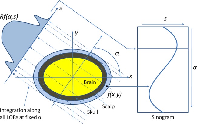
The schematic diagram of Radon transformation. The integration is along the line of response (LOR). Access the article online to view this figure in colour.

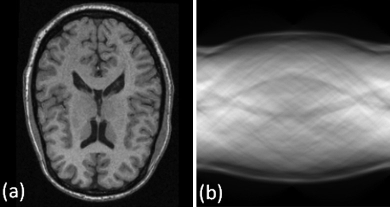
After the Radon transform, the MR image is transformed from the image domain to the Radon domain. Figure 2 shows the MR image and the corresponding sinogram in the Radon domain. On the sinogram image, the two, curved bands with low signal intensities on the top and bottom sides, correspond to the skull because it has relatively low signal intensities seen on the T1-weighted MR image.

Figure 2.

A T1-weighted MR image (A) and its corresponding sinogram (B).

Noise robustness

Radon transform is integration of signals along a line. When an MR image is added with white noise of zero mean, Radon transform of noises along the line will cancel each other. Radon transform can improve the signal-to-noise ratio (SNR) in the Radon domain. The improvement is demonstrated by the following brain model (figure 3). To simplify, the shape of the brain can be modeled as a circular area. As shown in the appendix, is increased by a factor of .

Figure 3.

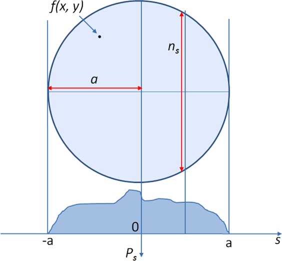
Brain ellipse model and the calculation scheme in the Radon domain. Access the article online to view this figure in colour.

Figure 4 illustrates the profiles from the original MR images and the corresponding sinograms. By adding 8% and 16% noise to the original MR images, the profiles become noisy and many details are not detectable. However, the profiles in the corresponding sinograms are relatively smooth. Before Radon transform, the SNRs are 28.2 dB and 14.4 dB for MR images with 8% and 16% added noise, respectively. After Radon transform, the SNRs are 69.5 dB and 55.9 dB for the sinogram data, respectively. Note that a rotation of the input image corresponds to the translation in the Radon domain which can be more suitable for segmentation.⁵³

Figure 4.

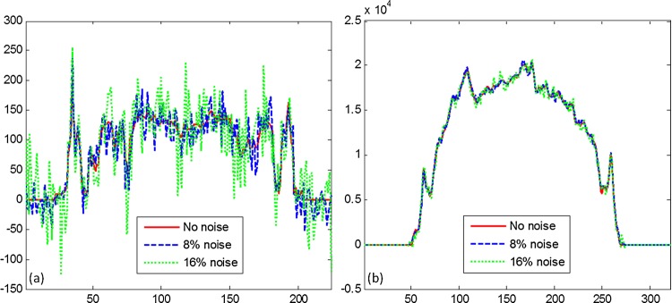
Comparison of profiles. (A) The profiles between the original and the noised MR images. (B) The profiles of the corresponding sinogram. Access the article online to view this figure in colour.

Multiscale space from bilateral filtering

Images in the multiscale space represent a series of images with different levels of spatial resolution. In the coarse scale, general information is maintained in the images while the images in the fine scale have more local tissue information. Bilateral filtering can introduce a partial edge detection step into the filtering process in order to simultaneously encourage intra-region smoothing and preserve the inter-region edge.

Bilateral filtering

Bilateral filtering is a non-linear filtering technique introduced by Tomasi.⁵⁴ This filter is a weighted average of the local neighborhood samples in which the weights are computed-based on the temporal (or spatial in the case of images) and radiometric distances between the center sample and the neighboring samples. This filter smoothes images while preserving image edges by means of a non-linear combination of nearby image values. Bilateral filtering can be described as follows:

2

with normalization that ensures that the weights for all the pixels add up to one.

3

where and denote input images and output images, respectively. We define that is the spatial function and is the range function. measures the geometric closeness between the neighborhood center and a nearby point and measures the photometric similarity between the pixel at the neighborhood center and that of a nearby point . Thus, the spatial function operates in the domain of , while the range function operates in the range of the image function . The bilateral filter replaces the pixel value at with an average of similar and nearby pixel values. In smooth regions, pixel values in a small neighborhood are similar to each other, and the bilateral filter acts essentially as a standard domain filter that averages away the small, weakly correlated differences between pixel values caused by noise.⁵⁵

Gaussian kernel

Many kernels can be used in bilateral filtering. A simple and important case of bilateral filtering is shift-invariant Gaussian filtering in which both the spatial function, and the range function, are Gaussian functions of the Euclidean distance between their arguments. More specifically, is described as:

4

where is the Euclidean distance. The range function, is similar to :

5

where is a measure of distance in the intensity space. In the scalar case, this may be simply the absolute difference of pixels. Both the spatial and the range filters are shift-invariant. The Gaussian range filter is insensitive to the overall additive changes of image intensity.

Multiscale bilateral decomposition

For an input discrete image, , the goal of the multiscale bilateral decomposition^56–58 is used to first build a series of filtered images, , that preserve the strongest edges in while smoothing small changes in intensity. Let the original image be the 0th scale , that is, set . By iteratively applying the bilateral filter as:

6

where is a pixel coordinate, , and are the widths of the spatial and range Gaussian functions, respectively, and is an offset relative to that runs across the support of the spatial Gaussian function. The repeated convolution by increases the spatial smoothing in each scale . In the finest scale, set the spatial kernel as . As the bilateral filter is non-linear, the filtered image is not identical to the one obtained by bilaterally filtering the original image, , with a spatial kernel of cumulative width.

The range Gaussian is an edge-stopping function. If an edge is strong enough to survive after several iterations of the bilateral decomposition, it should be preserved by setting . Increasing the width of the range Gaussian function by a factor of 2 in every scale increases the chance that an unwanted edge that survives at previous iterations will be smoothed away in later iterations. The initial width is set to be , where is the intensity range of the image.

Bilateral filtering smoothes the images as the scale increases. The original image is at the level of i=0. As the scale increases, the images become blurred and contain more general information. At the 5th and 6th scales, the images are smoothed and large edges are preserved. Unlike other multi-resolution techniques where the images are down-sampled along the resolution, bilateral filtering does not subsample the image because such down-sampling would blur the edges in . In addition, down-sampling would prevent the decomposition from becoming a translational invariant and could thus introduce grid artifacts when the coarser scales are manipulated.

In order to compare the difference in every scale, the horizontal profiles are computed through every scale. When the scale increases, small edges are smoothed in the intra-regions and large edges in the inter-regions are preserved. By controlling the scale number, the processing will preserve the needed edges but will smooth the image at the same time.

Gradient filtering and multiscale reconstruction

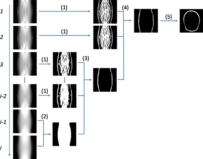
In each scale, images are filtered with two sets of filters, the kernels of which are shown in figure 5. The two kernels are mirrored along the vertical direction. They are applied to the same image. The upper half of the first filtered image is then combined with the lower half of the second filtered image. This step generates the images with edges along the vertical direction. The edge information will be used to detect the edge along the skull. This step is performed at multiple scales. In figure 6, step (1) shows the images and their corresponding images after the processing at different scales.

Figure 5.

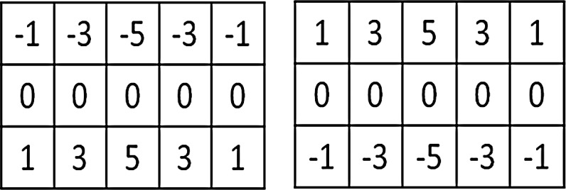
Kernels of the two filters.

Figure 6.

Illustration of the multiscale processing steps. From top to bottom, the scale increases from 1 to i. Based on the sinogram images after multiscale bilateral decomposition, the algorithm processes the images step by step from step (1) to step (4). Access the article online to view this figure in colour.

In the coarsest scale, the images are smoothed and only edges are preserved. For the two highest scales, a region-growing method⁵⁹ is used to obtain a ‘head’ mask, as shown in step (2) in figure 6. The region is iteratively grown by comparing all unallocated neighboring pixels to the region. The difference between a pixel's intensity value and the region's mean is used as a measure of similarity. This process stops when the intensity difference between region mean and the new pixel becomes larger than a certain threshold. In step 3, the head mask and the results from step (1) processing at the third to the (i − 2)th scales are combined to generate a ‘skull’ mask. In step (4), the skull mask and the results from step (1) processing in the first and second scales are used to generate the final sinogram of the skull. Step (5) is the reconstruction used in order to obtain the skull in the original MR image. The multiscale processing steps not only maintain the edge of the skull in the finest scale but also smooth the image at the coarse levels. The skull segmentation uses the combination of information from multiple scales in order to accurately delineate the skull on brain MR images.

Reconstruction

Reconstruction of the reciprocal binary sinogram is performed in order to obtain the skull on the original MR image. The reconstruction is described as

7

where is the ramp-filtered projections. In general, three, different inverse Radon transformation methods are the direct inverse Radon transform (DIRT), filtered back projection (FBP), and convolution FBP.⁶⁰ DIRT is computationally efficient but can introduce artifacts. FBP based on a linear filtering model often exhibits degradation when recovering from noisy data. Spline-convolution FBP (SCFBP) offers better approximation performance than the conventional lower-degree formulation, for example, piece-wise constant or piece-wise linear models.⁶¹ For SCFBP, the denoised sinogram in the Radon domain is approximated in the B-spline space, while the resulting image in the image domain is in the dual-spline space. We used SCFBP to propagate the segmented sinogram back into the image space along the projection paths.

Brain MR and CT image data for segmentation evaluation

We examined the segmentation results from pairs of CT and T1-weighted MRI data obtained from the Vanderbilt Retrospective Registration Evaluation Dataset.⁶² These CT and MR image volumes of the head were acquired preoperatively in human patients. Each image volume contains 40–45 transverse slices with 512×512 pixels. The voxel dimensions are approximately 0.4×0.4×3.0 mm³. The corresponding MR image volumes were acquired using a magnetization-prepared, rapid gradient-echo (MP-RAGE) sequence. Each image volume contains 128 coronal slices with 256×256 pixels. The voxel dimensions are approximately 1.0×1.0×1.6 mm³. The CT and MR images were registered using the registration methods that have been previously validated.^63–68 The skull was segmented from CT images using a Hounsfield value of approximately 600 as the threshold and the results served as the gold standard to evaluate the skull segmentation of the MR images.

Real PET data for attenuation correction

PET images were acquired from a dedicated high-resolution research tomograph (HRRT) system (Siemens, Knoxville, Tennessee, USA). This scanner used collimated single-photon point sources of 137Cs to produce high-quality transmission data as a consequence of higher count rates resulting from the decreased detector dead time and improved object penetration compared to conventional, positron-emitting transmission sources. The image size is 128×128×207 with a voxel size of 2.4×2.4×1.2 mm³. The reconstructed images are interpolated and consist of 207 slices with 256×256×207 voxels and with a voxel size of 1.2×1.2×1.2 mm³. Clinical brain PET scans of 10 patients who were referred to the Division of Nuclear Medicine and Molecular Imaging of Emory University Hospital for a study on Alzheimer's disease using ¹¹C-labeled Pittsburgh Compound-B, were selected from the database and were used for the clinical evaluation of the developed, segmentation-based AC method. Transmission (TX)-based AC is used as the gold standard to evaluate our segmented MRI-based method.

Qualitative and quantitative evaluation of the differences between the images processed using both the TX-based and the segmented MRI-based method were performed at the clinical volumes of interest (VOIs) (including regional cerebral metabolism). The images reconstructed using both processing methods were realigned to an anatomically standardized stereotactic template using our registration algorithm⁶⁹ and with a rigid body transformation for the VOIs. Seventeen VOIs were defined in different slices of the MRI template and were superimposed on each scan, thus resulting in a total of 170 VOIs for the 10 patients. The registered PET images were then used for quantitative analysis of the defined VOIs. The VOIs included left cerebellum (LCE), left cingulate, left calcarine sulcus, left frontal lobe, left lateral temporal, left medial temporal (LMT), left occipital lobe (LOL), left parietal lobe, pons (PON), right cerebellum (RCE), right cingulate (RCI), right calcarine sulcus, right frontal lobe, right lateral temporal, right medial temporal (RMT), right occipital lobe (ROL), and right parietal lobe. The LMT and RMT regions included the amygdale, hippocampus, and the entorhinal cortex.

Segmentation evaluation

In order to evaluate the performance of the segmentation method, the difference between the segmented images and the ground truth was computed using a variety of quantitative evaluation methods. The ground truth is established by manual segmentation in real patient data. We defined six metrics in order to evaluate the segmentation results. The overlap ratios, C₁,⁵⁰ C₂, and C₃, and the error ratios, E₁, E₂, and E₃, were defined as follows.

8

and

9

where S₁ is the ground truth, and S₂ is the segmented result using our method. Both S₁ and S₂ are binary images.

Results

Segmentation experiments were performed using brain phantom data, simulated MR images from the McGill phantom brain database, human patient MR and CT images from the Vanderbilt dataset, and real patient MR images. The study was approved by our Institutional Review Board (IRB) and was compliant with the Health Insurance Portability and Accountability Act.

Brian phantom results

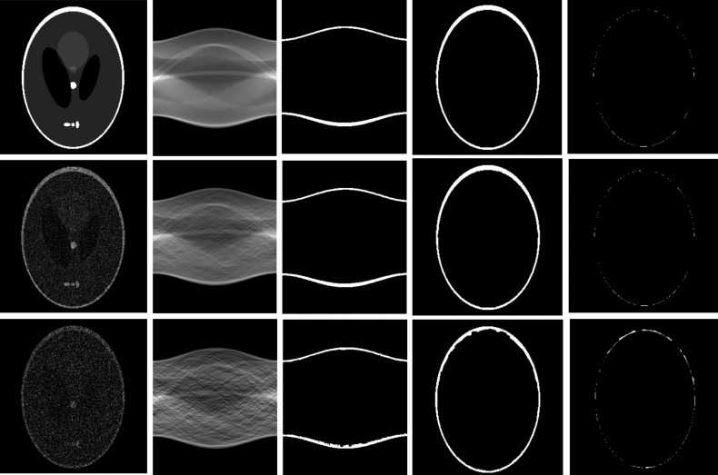
Figure 7 shows the results from the brain phantom images. In order to compare the results, noise at the level of 40% or 80% of the maximum intensity was added to the original brain phantom images. The proposed method is able to accurately segment the skull in the simulated brain data. It is also robust to noise at the level of 80% of the maximum intensity. The difference between the segmented and the ground truth is minimal, partially due to the interpolation errors made during reconstruction.

Figure 7.

Segmentation results of brain phantoms at different noise levels. From left to right, simulated brain image, sinogram data, segmented signogram, reconstructed skull, and different images between the segmented skull and the ground truth. From top to bottom, image without noise, that with 40% noise, and that with 80% noise.

Quantitative evaluation results showed that the segmentation method is not sensitive to noise. The overlap ratios are greater than 93.3% when the noise level is equal to or less than 50% of the maximum intensity. When the noise level is increased to 100%, the overlap ratios are 82.6%±2.1%, thus indicating that the segmentation method is robust to noisy images. The error ratios are less than 5% when the noise levels are equal to or less than 30%.

MR and CT images from the Vanderbilt Dataset

The different images from the CT- and MRI-based segmentation show only a minimal difference, which indicates that the MR segmentation is close to the CT segmentation of the skull. Quantitative evaluation shows that the lowest overlap ratio, that is, C1, is 85.2%±2.6%. The highest error ratio, that is, E3, is 18.0%±3.2%. The MRI-based segmentation is therefore close to the CT-based segmentation of the skull.

AC results on clinical PET data

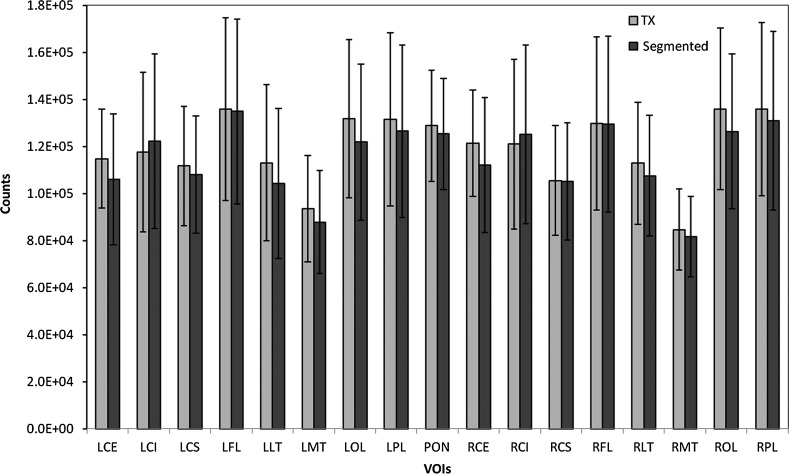
Figure 8 illustrates the means as well as SDs resulting from the quantitative analysis for both methods in each of the 17 VOIs, and averaged across the 10 patients. The relative difference between the TX-based and the MRI-based AC methods was calculated for the VOIs estimate using the TX-based method as the reference. The maximum difference between the two methods is less than 8%.

Figure 8.

Regional cerebral metabolism estimates are shown for the 17 volumes of interest (VOIs). Means and SDs are calculated across the 10 patients studied. TX, transmission.

Discussion and conclusion

We developed and evaluated a multiscale skull segmentation method for MR images. T1-weighted MR images are transformed to the Radon domain in order to detect the skull features on the images. In the Radon domain, a bilateral filter is proposed to simultaneously attenuate noise and to preserve edge information. Two kernels are used to filter images at different scales. The width of the range and spatial Gaussian functions are increased by a factor of 2 as the scale increases. By processing edge and mask information from the coarse to fine scales, the skull is extracted in the MR sinogram data. After reconstruction, the skull is segmented on the original MR images.

One unique feature of our method is that the algorithm is robust for MR images with random noises. Our particular contribution is that the segmentation algorithm includes the use of the Radon transform and bilateral filtering. Radon transform can improve the signal-to-noise ratio while bilateral filtering simultaneously keeps the edge information and smoothes noise. The multiscale decomposition technique makes our segmentation reliable; it also improves the robustness and speed of the segmentation method.

As the skull segmentation was performed in the Radon space, it has advantages over the image space for this application. In low-intensity regions such as the skull and CSF in T1-weighted images, the noise level is high, which can affect the segmentation accuracy of skull when the skull is segmented in the image domain using intensity-based methods or boundary-based methods. As the intensities of CSF and skull are similar, it can be difficult for region-based, boundary-based, or intensity-based methods to accurately segment the skull. By transferring the images from the image domain to the Radon domain, our method improves the SNR and potentially eliminates the effect of CSF on the skull segmentation.

There is a limitation to our segmentation method when applying it to MR-based AC. For T1-weighted MR images, the segmentation method can have difficulty differentiating bone and air as both have a low MR signal intensity. The accuracy of bone segmentation can be affected in areas where the sinuses are located. This is particularly true for transverse slices located below the eyes. We therefore gave the same attenuation coefficient of 0.096 for the slices below eyes in our segmentation-based AC method. We used 17 VOIs to evaluate our segmentation-based AC results. The maximum difference between the TX-based AC method and our segmentation-based AC method is less than 8%. Because the AC map did not include air, it overestimated (over-corrected) some regions such as LCE, RCE, LOL, and ROL. For MR images that are acquired UTE sequences, this issue can be resolved as bone will be shown on UTE MR images. The segmentation method has been integrated into the quantification tools for combined MR/PET applications.⁷⁰ The segmentation method can also be used in other neuroimaging applications.

As an emerging imaging modality, integrated MR/PET holds great potential for brain research, especially for multi-parametric analysis of complex function in neuronal networks.⁷¹ An integrated MR/PET system will permit the simultaneous acquisition of several imaging parameters. Quantitative values from PET of a large number of biological parameters are complemented by the high-resolution information provided by MRI to yield complementary information of previously unexpected variability. The combination of imaging modalities for high sensitivity and high resolution with the additional advantage of utilizing dynamic acquisition procedures appears very appealing for a variety of brain clinical and research applications. Recently, PET and MRI data have been retrospectively combined for detection and staging of gliomas as well as for identification of areas with critical neurofunction in the vicinity of tumors, which is important for planning surgery. Combined MR/PET has gained a place in the early diagnosis of dementia and mild cognitive impairment and degenerative disorders, for example, cerebral atrophy and Huntington chorea. Combined MR/PET is of clinical value in the detection of epileptic foci accessible for surgery and for the identification of metabolic activity, transmitter concentration and enzyme expression in small brain structures. The MR-based attenuation correction is critical for quantitative MR/PET imaging that will have various applications in both research and clinical studies. Multimodality imaging such as PET and MRI can provide both functional and anatomic information for a variety of research and clinical applications. By combing radiologic imaging information with other health information such as pathology and tissue genomic information, biomedical imaging informatics has the potential to advance future personalized medicine.

Appendix

SNR after Radon transformation

Radon transform is integration of signals along a line. When an MR image is added with white noise of zero mean, Radon transform of noises along the line will cancel each other. Radon transform can improve the SNR in the Radon domain. The improvement is demonstrated by the brain model (figure 3). The shape of the brain can be modeled as a circular area.

Radon transform sums the intensity values of the pixels along the line. Assume that is a 2-D discrete signal whose intensity values have a mean of and variance of . Then for each point along the projection, add up pixels of . The mean will be described by , and the variance is described by . Here,, and is the radius of the circular area in terms of pixels and the integer s is the projection index which varies from to .

The average of is

rmA1

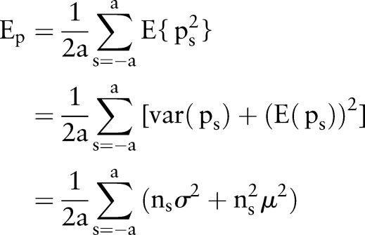
Its expected value is defined as . Then

rmA2

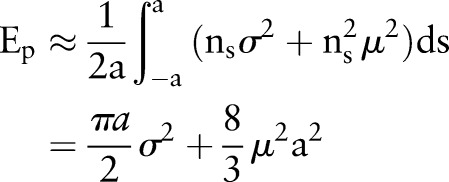
For a large we can get

rmA3

For the signal s, . For Gaussian white noise with zero mean and with a variance of , . The signal-to-noise ratio in the Radon domain can be calculated as

rmA4

In the original MR image, the signal-to-noise ratio can be defined as .

rmA5

In real MR images , hence ,

rmA6

In high-resolution MR images, we assume .

rmA7

rmA8

Since , . Hence, after Radon transformation, is increased by a factor of .

References

- 1.Sauter AW, Wehrl HF, Kolb A, et al. Combined PET/MRI: one step further in multimodality imaging. Trends Mol Med 2010;16:508–15 [DOI] [PubMed] [Google Scholar]
- 2.Zaidi H, Montandon ML, Slosman DO. Magnetic resonance imaging-guided attenuation and scatter corrections in three-dimensional brain positron emission tomography. Med Phys 2003;30:937–48 [DOI] [PubMed] [Google Scholar]
- 3.Fei B, Yang X, Wang H. An MRI-based attenuation correction method for combined PET/MRI applications. SPIE medical imaging—biomedical applications: molecular, structural, and functional imaging. In: Hu XP, Clough AV, eds. Proceedings of SPIE; 2009:726208. [DOI] [PMC free article] [PubMed] [Google Scholar]
- 4.Schulz V, Torres-Espallardo I, Renisch S, et al. Automatic, three-segment, MR-based attenuation correction for whole-body PET/MR data. Eur J Nucl Med Mol Imaging 2011;38:138–52 [DOI] [PubMed] [Google Scholar]
- 5.Kops ER, Wagenknecht G, Scheins J, et al. Attenuation correction in MR-PET scanners with segmented T1-weighted MR images. In: Yu B, ed. 2009 IEEE Nuclear Science Symposium Conference Record; Vol 1–5, 2009:2530–3 [Google Scholar]
- 6.Montandon ML, Zaidi H. Quantitative analysis of template-based attenuation compensation in 3D brain PET. Comput Med Imaging Graph 2007;31:28–38 [DOI] [PubMed] [Google Scholar]
- 7.Hofmann M, Steinke F, Scheel V, et al. MRI-based attenuation correction for PET/MRI: a novel approach combining pattern recognition and atlas registration. J Nucl Med 2008;49:1875–83 [DOI] [PubMed] [Google Scholar]
- 8.Beyer T, Weigert M, Quick HH, et al. MR-based attenuation correction for torso-PET/MR imaging: pitfalls in mapping MR to CT data. Eur J Nucl Med Mol Imaging 2008;35:1142–6 [DOI] [PubMed] [Google Scholar]
- 9.Catana C, van der KA, Benner T, et al. Toward implementing an MRI-based PET attenuation-correction method for neurologic studies on the MR-PET brain prototype. J Nucl Med 2010;51:1431–8 [DOI] [PMC free article] [PubMed] [Google Scholar]
- 10.Keereman V, Fierens Y, Broux T, et al. MRI-based attenuation correction for PET/MRI using ultrashort echo time sequences. J Nucl Med 2010;51:812–18 [DOI] [PubMed] [Google Scholar]
- 11.Berker Y, Franke J, Salomon A, et al. MRI-based attenuation correction for hybrid PET/MRI systems: a 4-class tissue segmentation technique using a combined ultrashort-echo-time/dixon MRI sequence. J Nucl Med 2012;53:796–804 [DOI] [PubMed] [Google Scholar]
- 12.Tsai C, Manjunath BS, Jagadeesan B. Automated segmentation of brain MR images. Pattern Recognit 1995;28:1825–37 [Google Scholar]
- 13.van Ginneken B, Frangi AF, Staal JJ, et al. Active shape model segmentation with optimal features. IEEE Trans Med Imaging 2002;21:924–33 [DOI] [PubMed] [Google Scholar]
- 14.Grau V, Mewes AUJ, Alcaniz M, et al. Improved watershed transform for medical image segmentation using prior information. IEEE Trans Med Imaging 2004;23:447–58 [DOI] [PubMed] [Google Scholar]
- 15.Poynton C, Chonde D, Sabunca M, et al. Atlas-based segmentation of T1-weighted and Dute MRI for calculation of attenuation correction maps in PET-MRI of brain tumor patients. J Nucl Med 2012;53(MeetingAbstracts):2332 [Google Scholar]
- 16.Wang H, Feyes D, Mulvihil J, et al. Multiscale fuzzy C-means image classification for multiple weighted MR images for the assessment of photodynamic therapy in mice. In: Josien PW, Pluim JMR, eds. SPIE Medical Imaging: Image Processing; Proceedings of SPIE; Vol. 6512, 2007:65122W. [DOI] [PMC free article] [PubMed] [Google Scholar]
- 17.Wang HS, Fei BW. A modified fuzzy C-means classification method using a multiscale diffusion filtering scheme. Med Image Anal 2009;13:193–202 [DOI] [PMC free article] [PubMed] [Google Scholar]
- 18.Yang XF, Fei BW. A multiscale and multiblock fuzzy C-means classification method for brain MR images. Med Phys 2011;38:2879–91 [DOI] [PMC free article] [PubMed] [Google Scholar]
- 19.Segonne F, Dale AM, Busa E, et al. A hybrid approach to the skull stripping problem in MRI. NeuroImage 2004;22:1060–75 [DOI] [PubMed] [Google Scholar]
- 20.Atkins MS, Mackiewich BT. Fully automatic segmentation of the brain in MRI. IEEE Trans Med Imaging 1998;17:98–107 [DOI] [PubMed] [Google Scholar]
- 21.Cox RW. AFNI: software for analysis and visualization of functional magnetic resonance neuroimages. Comput Biomed Res 1996;29:162–73 [DOI] [PubMed] [Google Scholar]
- 22.Lemieux L, Hagemann G, Krakow K, et al. Fast, accurate, and reproducible automatic segmentation of the brain in T1-weighted volume MRI data. Magn Reson Med 1999;42:127–35 [DOI] [PubMed] [Google Scholar]
- 23.Rifa H, Bloch I, Hutchinson S, et al. Segmentation of the skull in MRI volumes using deformable model and taking the partial volume effect into account. Med Image Anal 2000;4:219–33 [DOI] [PubMed] [Google Scholar]
- 24.Dale AM, Fischl B, Sereno MI. Cortical surface-based analysis. I. Segmentation and surface reconstruction. NeuroImage 1999;9:179–94 [DOI] [PubMed] [Google Scholar]
- 25.Smith SM. Fast robust automated brain extraction. Hum Brain Mapp 2002;17:143–55 [DOI] [PMC free article] [PubMed] [Google Scholar]
- 26.MacDonald D, Kabani N, Avis D, et al. Automated 3-D extraction of inner and outer surfaces of cerebral cortex from MRI. NeuroImage 2000;12:340–56 [DOI] [PubMed] [Google Scholar]
- 27.Shattuck DW, Sandor-Leahy SR, Schaper KA, et al. Magnetic resonance image tissue classification using a partial volume model. NeuroImage 2001;13:856–76 [DOI] [PubMed] [Google Scholar]
- 28.Baillard C, Hellier P, Barillot C. Segmentation of brain 3D MR images using level sets and dense registration. Med Image Anal 2001;5:185–94 [DOI] [PubMed] [Google Scholar]
- 29.Ghadimi S, Abrishami-Moghaddam H, Kazemi K, et al. Segmentation of scalp and skull in neonatal MR images using probabilistic atlas and level set method. Conf Proc IEEE Eng Med Biol Soc 2008:3060–3 [DOI] [PubMed] [Google Scholar]
- 30.Zhuang AH, Valentino DJ, Toga AW. Skull-stripping magnetic resonance brain images using a model-based level set. NeuroImage 2006;32:79–92 [DOI] [PubMed] [Google Scholar]
- 31.DeCarli C, Maisog J, Murphy DG, et al. Method for quantification of brain, ventricular, and subarachnoid CSF volumes from MR images. J Comput Assist Tomogr 1992;16:274–84 [DOI] [PubMed] [Google Scholar]
- 32.Shan ZY, Yue GH, Liu JZ. Automated histogram-based brain segmentation in T1-weighted three-dimensional magnetic resonance head images. NeuroImage 2002;17:1587–98 [DOI] [PubMed] [Google Scholar]
- 33.Lee C, Huh S, Ketter TA, et al. Unsupervised connectivity-based thresholding segmentation of midsagittal brain MR images. Comput Biol Med 1998;28:309–38 [DOI] [PubMed] [Google Scholar]
- 34.Stokking R, Vincken KL, Viergever MA. Automatic morphology-based brain segmentation (MBRASE) from MRI-T1 data. NeuroImage 2000;12:726–38 [DOI] [PubMed] [Google Scholar]
- 35.Huh S, Ketter TA, Sohn KH, et al. Automated cerebrum segmentation from three-dimensional sagittal brain MR images. Comput Biol Med 2002;32:311–28 [DOI] [PubMed] [Google Scholar]
- 36.Dogdas B, Shattuck DW, Leahy RM. Segmentation of skull and scalp in 3-D human MRI using mathematical morphology. Hum Brain Mapp 2005;26:273–85 [DOI] [PMC free article] [PubMed] [Google Scholar]
- 37.Chiverton J, Wells K, Lewis E, et al. Statistical morphological skull stripping of adult and infant MRI data. Comput Biol Med 2007;37:342–57 [DOI] [PubMed] [Google Scholar]
- 38.Kapur T, Grimson WE, Wells WM, III, et al. Segmentation of brain tissue from magnetic resonance images. Med Image Anal 1996;1:109–27 [DOI] [PubMed] [Google Scholar]
- 39.Xiaolan Z, Staib LH, Schultz RT, et al. Volumetric layer segmentation using coupled surfaces propagation. Proceedings of IEEE Computer Society Conference on Computer Vision and Pattern Recognition; 1998:708–15 [Google Scholar]
- 40.Aboutanos GB, Nikanne J, Watkins N, et al. Model creation and deformation for the automatic segmentation of the brain in MR images. IEEE Trans Biomed Eng 1999;46:1346–56 [DOI] [PubMed] [Google Scholar]
- 41.Duncan JS, Ayache N. Medical image analysis: progress over two decades and the challenges ahead. IEEE Trans Pattern Anal Mach Intell 2000;22:85–106 [Google Scholar]
- 42.Rehm K, Schaper K, Anderson J, et al. Putting our heads together: a consensus approach to brain/non-brain segmentation in T1-weighted MR volumes. NeuroImage 2004;22:1262–70 [DOI] [PubMed] [Google Scholar]
- 43.Rex DE, Shattuck DW, Woods RP, et al. A meta-algorithm for brain extraction in MRI. NeuroImage 2004;23:625–37 [DOI] [PubMed] [Google Scholar]
- 44.Pohl KM, Fisher J, Kikinis R, et al. Shape based segmentation of anatomical structures in magnetic resonance images. Lect Notes Comput Sc 2005;3765:489–98 [DOI] [PMC free article] [PubMed] [Google Scholar]
- 45.Carass A, Wheeler MB, Cuzzocreo J, et al. A joint registration and segmentation approach to skull stripping. I S Biomed Imaging 2007;2007:656–9 [Google Scholar]
- 46.Soltanian-Zadeh H, Windham JP. A multiresolution approach for contour extraction from brain images. Med Phys 1997;24:1844–53 [DOI] [PubMed] [Google Scholar]
- 47.Akahn Z, Acar CE, Gencer NG. Development of realistic head models for electromagnetic source imaging of the human brain. Proceedings of the 23rd Annual International Conference of the IEEE Engineering in Medicine and Biology Society; Vol. 1, 2001:899–902 [Google Scholar]
- 48.Kovacevic N, Lobaugh NJ, Bronskill MJ, et al. A robust method for extraction and automatic segmentation of brain images. NeuroImage 2002;17:1087–100 [DOI] [PubMed] [Google Scholar]
- 49.Tyler DJ, Robson MD, Henkelman RM, et al. Magnetic resonance imaging with ultrashort TE (UTE) PULSE sequences: technical considerations. J Magn Reson Imaging 2007;25:279–89 [DOI] [PubMed] [Google Scholar]
- 50.Fennema NC, Ozyurt IB, Clark CP, et al. Quantitative evaluation of automated skull-stripping methods applied to contemporary and legacy images: effects of diagnosis, bias correction, and slice location. Hum Brain Mapp 2006;27:99–113 [DOI] [PMC free article] [PubMed] [Google Scholar]
- 51.Boesen K, Rehm K, Schaper K, et al. Quantitative comparison of four brain extraction algorithms. NeuroImage 2004;22:1255–61 [DOI] [PubMed] [Google Scholar]
- 52.Amato U, Larobina M, Antoniadis A, et al. Segmentation of magnetic resonance brain images through discriminant analysis. J Neurosci Methods 2003;131:65–74 [DOI] [PubMed] [Google Scholar]
- 53.Yang XF, Fei BW. A wavelet multiscale denoising algorithm for magnetic resonance (MR) images. Meas Sci Technol 2011;22:025803. [DOI] [PMC free article] [PubMed] [Google Scholar]
- 54.Tomasi C, Manduchi R. Bilateral filtering for gray and color images. Sixth International Conference on Computer Vision 1998:839–46 [Google Scholar]
- 55.Elad M. On the origin of the bilateral filter and ways to improve it. IEEE Trans Image Process 2002;11:1141–51 [DOI] [PubMed] [Google Scholar]
- 56.Fattal R, Agrawala M, Rusinkiewicz S. Multiscale shape and detail enhancement from multi-light image collections. Acm Trans Graph 2007;26:51–9 [Google Scholar]
- 57.Yang XF, Wu SY, Sechopoulos I, et al. Cupping artifact correction and automated classification for high-resolution dedicated breast CT images. Med Phys 2012;39:6397–406 [DOI] [PMC free article] [PubMed] [Google Scholar]
- 58.Yang XF, Sechopoulos I, Fei BW. Automatic tissue classification for high-resolution breast CT images based on bilateral filtering. Proceedings of SPIE; Vol. 7962:79623H. [DOI] [PMC free article] [PubMed] [Google Scholar]
- 59.Pham DL, Xu CY, Prince JL. Current methods in medical image segmentation. Annu Rev Biomed Eng 2000;2:315. [DOI] [PubMed] [Google Scholar]
- 60.Yazgan B, Paker S, Kartal M. Image reconstruction with diffraction tomography using different inverse Radon transform algorithms. Proceedings of the International Biomedical Engineering Days; August 1992:170–3 [Google Scholar]
- 61.Horbelt S, Liebling M, Unser M. Discretization of the radon transform and of its inverse by spline convolutions. IEEE Trans Med Imag 2002;21:363–76 [DOI] [PubMed] [Google Scholar]
- 62.West J, Fitzpatrick JM, Wang MY, et al. Comparison and evaluation of retrospective intermodality brain image registration techniques. J Comput AssistTomogr 1997;21:554–66 [DOI] [PubMed] [Google Scholar]
- 63.Fei B, Lee S, Boll D, et al. Image registration and fusion for interventional MRI guided thermal ablation of the prostate cancer. In: Ellis RE, Peters TM, eds. Lecture Notes in Computer Science (LNCS) The 6th International Conference on Medical Image Computing and Computer-Assisted Intervention (MICCAI 2003), 2003;2879:364–72. [Google Scholar]
- 64.Fei B, Kemper C, Wilson D. Three-dimensional warping registration of the pelvis and prostate. In: Sonka M, Fitzpatrick JM, eds. SPIE Medical Imaging: Image Processing, Proceedings of SPIE; Vol. 4684, 2002:528–37 [Google Scholar]
- 65.Fei B, Wang H, Muzic RF, et al. Deformable and rigid registration of MRI and microPET images for photodynamic therapy of cancer in mice. Med Phys 2006;33:753–60 [DOI] [PubMed] [Google Scholar]
- 66.Fei B, Lee Z, Duerk JL, et al. Registration and fusion of SPECT, high resolution MRI, and interventional MRI for thermal ablation of the prostate cancer. IEEE Trans Nucl Sci 2004;51:177–83 [Google Scholar]
- 67.Fei BW, Duerk JL, Sodee DB, et al. Semiautomatic nonrigid registration for the prostate and pelvic MR volumes. Acad Radiol 2005;12:815–24 [DOI] [PubMed] [Google Scholar]
- 68.Bogie K, Wang X, Fei B, et al. New technique for real-time interface pressure analysis: getting more out of large image data sets. J Rehabil Res Dev 2008;45:523–35 [DOI] [PMC free article] [PubMed] [Google Scholar]
- 69.Fei B, Wang H, Muzic RF, Jr, et al. Deformable and rigid registration of MRI and microPET images for photodynamic therapy of cancer in mice. Med Phys 2006;33:753. [DOI] [PubMed] [Google Scholar]
- 70.Fei B, Yang X, Nye JA, et al. MR/PET quantification tools: registration, segmentation, classification, and MR-based attenuation correction. Med Phys 2012;39:6443–54 [DOI] [PMC free article] [PubMed] [Google Scholar]
- 71.Heiss WD. The potential of PET/MR for brain imaging. Eur J Nucl Med Mol I 2009;36:105–12 [DOI] [PubMed] [Google Scholar]