NP-MuScL: Unsupervised Global Prediction of Interaction Networks from Multiple Data Sources

Abstract

Inference of gene interaction networks from expression data usually focuses on either supervised or unsupervised edge prediction from a single data source. However, in many real world applications, multiple data sources, such as microarray and ISH (in situ hybridization) measurements of mRNA abundances, are available to offer multiview information about the same set of genes. We propose ISH to estimate a gene interaction network that is consistent with such multiple data sources, which are expected to reflect the same underlying relationships between the genes. NP-MuScL casts the network estimation problem as estimating the structure of a sparse undirected graphical model. We use the semiparametric Gaussian copula to model the distribution of the different data sources, with the different copulas sharing the same precision (i.e., inverse covariance) matrix, and we present an efficient algorithm to estimate such a model in the high-dimensional scenario. Results are reported on synthetic data, where NP-MuScL outperforms baseline algorithms significantly, even in the presence of noisy data sources. Experiments are also run on two real-world scenarios: two yeast microarray datasets and three Drosophila embryonic gene expression datasets, where NP-MuScL predicts a higher number of known gene interactions than existing techniques.

1. Introduction

With the prevalence of high-throughput technologies such as microarray and RNA-seq for measuring gene expressions, computational inference of gene regulatory or interaction networks from large-scale gene expression datasets has emerged as a popular technique to improve our understanding of cellular systems (Segal et al., 2003; Basso et al., 2005; Morrissey et al., 2010). In numerous studies, gene interactions reverse-engineered from analysis of such high-throughput data have been experimentally validated (Carro et al., 2010; Wang et al., 2009), demonstrating the credibility of such data-driven algorithmic approaches.

There have been two popular approaches to reverse-engineering gene networks. The first approach is to build a generative model of the data and learn a graphical model that captures the conditional independencies in the data. Learning the structure of a graphical model under a multivariate Gaussian assumption of the data has received wide attention in recent years (Meinshausen and Bühlmann, 2006; Banerjee et al., 2006; Friedman et al., 2007); various algorithms have been proposed (Meinshausen and Bühlmann, 2006; Banerjee et al., 2006; Friedman et al., 2007), many with theoretical analysis offering asymptotic guarantee of consistent estimation of the interactions between genes in the network. Empirically, these algorithms are computationally efficient, and the results obtained have been encouraging.

However, a limitation of this class of network inference approach is that it assumes data are identically and independently distributed (i.e., iid), which implicitly means that they are from a single experimental source. In reality, many real-world biological problems sit on multiple sources of information that can be used to predict interactions between genes. For example, there can be multiple microarray datasets from different laboratories available for the same organism, sometimes measured at the same conditions in which the main differences lie in the data-sampling strategy or measurement technologies. Biologically, it is often plausible to assume that multiple experimental means resulting in the different datasets may have captured the same information from different viewpoints, for example, both microarray and in situ hybridization can capture gene expression information, even though the technology used to measure mRNA abundances is different. It remains unclear how to integrate such multiple sources of data in a statistically valid and computationally efficient way to infer the underlying network. One may imagine inferring independently a network from each data source and then averaging across multiple resultant networks, but such an ad hoc method is not only unrobust (e.g., each view may have only a small amount of samples), but also lacks statistical justification and consistence guarantee (e.g., on the “average” operator). In this article, we address the question of inferring a network by analyzing multiple sources of information simultaneously.

An alternative approach to tackle this problem is via supervised learning methods, where a classifier (e.g., SVM) is trained by using examples of known gene interactions (edges in the network) as training data to learn the importance of each data source in predicting unknown interactions between other gene-pairs (Ben-Hur and Noble, 2005). This approach suffers from some intrinsic limitations that prevent it from being widely applicable. First, while such an approach works well for problems in which there are sufficient examples of known edges in the network, for example, in the form of a reference network or reference interactions obtained from reliable sources, it fails for problems in which few or no examples of known edges are available. Gene networks for humans or yeast may be learned by supervised methods in which reference interactions are available from extensive prior studies, but for organisms where prior research is limited, this approach cannot be used. Furthermore, one can argue that predicting gene networks is of high importance for such organisms with few known edges, to help biologists who are starting to research regulatory mechanisms of these organisms.

Secondly, using a classifier to predict edges implicitly utilizes the notion of marginal independence between nodes. To classify an edge as “positive,” that is to predict an edge between a given pair of nodes, the correlation between the data for these nodes must be high. Gene networks usually have pathways in which genes interact with each other in a sequential order, which results in high marginal correlation between all pairs of genes in the same pathway. Predicting each edge locally and independently of all other edges will often result in a non stringent prediction of a clique for all genes in the same pathway, leading to high false-positive rates. To reduce such false-positives and increase accuracy, we aim to analyze conditional independence between the genes instead, which must be done by building a global graphical model that captures simultaneously all the conditional independencies among genes. Thus, conditional independence predicts an interaction between two genes in the context of all the other genes in the network, unlike marginal independence, which takes into account only the localized interaction between the genes without taking into account the other genes that may also be interacting with the given pair of genes. Each edge resultant from such an estimator enjoys global statistical interpretability and consistency guarantee, and such an estimator does not require supervised training, although prior knowledge of interactions on the “reference gene pairs” can still be utilized via introducing a prior over the model, if desired. Thus, it is desirable to develop an unsupervised and global inference method that can incorporate multiple data sources to predict a consensus graphical model that explains all the data sources, without using any examples of known edges for training the model.

This article proposes NP-MuScL (nonparanormal multi-source learning), a machine-learning technique for estimating the structure of a sparse undirected graphical model that is consistent with multiple sources of data. The multiple data sources are all defined over the same feature space, and it is assumed that they share the same underlying relationships between the genes (nodes). We use the semiparametric Gaussian copula to model the distribution of the different data sources, where the copula for each data source has its own mean and transformation functions, but all data sources share the same precision matrix (that is, the inverse covariance matrix, which captures the topological structure of the network). We propose an efficient algorithm to estimate such a model in the high-dimensional scenario. The likelihood-related objective function used in NP-MuScL is convex and results in a globally optimal estimator. Furthermore, the implementation of our algorithm is simple and efficient, computing a network over 2000 nodes using three data sources in a matter of minutes. Results are reported on synthetic data, where NP-MuScL outperforms baseline algorithms significantly, even in the presence of noisy data sources. We also use NP-MuScL to estimate a gene network for yeast using two microarray datasets: one over time-series expression, and the other over knockout mutants. Finally, we run NP-MuScL on three datasets of Drosophila embryonic gene expression using ISH images and microarray. In both yeast and Drosophila, we find that NP-MuScL predicts a higher number of gene interactions, which are known in the literature to interact than existing techniques.

1.1. Related work

Previous work on analyzing multiple data sources for network prediction has either specifically taken time into account (Wang et al., 2006; Ahmed and Xing, 2009) or has different source and target organisms via transfer learning (Xu et al., 2012). Katenka and Kolaczyk (2012) and Kolar et al. (2013) propose a strategy to learn a network from multiattribute data, where aligned vector observations are made for each node. The NP-MuScL algorithm, on the other hand, works for data sources that are not aligned, hence each data source may have a different number of observations. Honorio and Samaras (2011) and Danaher et al. (2013) proposed techniques for multitask structure learning of Gaussian graphical models, to share knowledge across multiple problems, using multitask learning and fused lasso or group lasso penalties respectively. However, their method estimates a separate graphical model for each data source, unlike our problem, which requires a consensus network common to all data sources. To the best of our knowledge, the NP-MuScL algorithm is the first work that builds a consensus graphical model to explain the relationship between genes by combining information from multiple data sources without explicitly constraining the data to be time-series or about different organisms.

2. Nonparanormal Multi-Source Learning (NP-MuScL)

Let the k input data sources be defined as with total number of data samples . Each data source i may have a different number of measurements or samples n_i, but they all measure information about the same feature space of d genes. The goal of NP-MuScL is to learn the structure of a graphical model over the feature space, such that the graphical model will encapsulate global conditional independencies between the genes.

2.1. Glasso

Given a single source of data drawn from a Gaussian distribution , a Gaussian graphical model (GGM) may be estimated by computing the inverse covariance matrix Σ⁻¹ of the Gaussian. Zeros in the inverse covariance matrix imply conditional independence between the features, and thus the absence of an edge between them in the corresponding GGM. Given the empirical covariance matrix S of the data, the inverse covariance matrix may be computed by maximizing the log likelihood of the data, with an L₁ regularizer to encourage sparsity.

(1)

where λ is a tuning parameter that controls the sparsity of the solution; as λ increases, fewer edges are predicted in the GGM. Rothman et al. (2008) showed the consistence of such estimators in Frobenius and Operator norms in high dimensions when d ≫ n. Friedman et al. (2007) proposed a block coordinate descent algorithm for this objective, they named their technique glasso. The glasso algorithm uses a series of L₁ penalized regressions, called Lasso regressions (Tibshirani, 1996), that can be solved in time O(d³).

2.2. Joint estimation of the GGM

Given k data sources with corresponding sample covariances , a joint estimator of the underlying GGM may be computed as

(2)

where w_i defines the relative importance of each data source and must be defined by the user such that . Assuming the data in each data source is drawn i.i.d., an appropriate choice for the weights may be . It can be seen that if each data source is assumed to have mean 0, then for this choice of w_i

(3)

Thus, our objective function is equivalent to calling glasso with covariance matrix . We call this method “glasso-bag of data.” With an appropriate choice of weights, this model concatenates the data from all data sources into a single matrix and uses the second moment of the data to estimate the inverse covariance matrix.

Such a procedure highlights the underlying assumption of Gaussianity of the data. If we assume that all data is being drawn from the same Gaussian distribution, then it is reasonable to construct a single sample covariance matrix from the data to estimate the network. However, real data is not always Gaussian, and such an assumption can be limiting, especially when analyzing multiple data sources simultaneously, since non-Gaussianity in a single data source will result in the non-Gaussianity of the combined data. A lot of previous work has been done to drop the Gaussianity assumption in the solution to classic problems like sparse regression (Ravikumar et al., 2007), estimating GGMs (Liu et al., 2009), sparse CCA (Balakrishnan et al., 2012), etc., and propose nonparametric solutions to the same. We will also drop the assumption that the data is drawn from the same Gaussian distribution in the next section.

However, if the data is not drawn from the same Gaussian distribution, then how can we characterize the underlying network that generated the data? We propose a generative model in which we assume that each data source is drawn from a semi-parametric Gaussian copula, where the copulas for the different data sources share the same covariance matrix but have different functional transformations. To justify this model, we assume that for each data source, the data is sampled from a multivariate Gaussian, but this sample is not directly observed. Instead, due to nonlinearities introduced during data measurement, a transformed version of the data is measured. Each data source will have its own transformation; hence, the observed distribution of each data source will be different. The key idea of NP-MuScL is then to estimate the nonlinear transformation so that all data can be assumed Gaussian, and the network can be estimated using Equation 2.

2.3. Dropping the Gaussianity assumption

We model that each data source is drawn from an underlying Gaussian distribution with mean 0 and covariance matrix Σ, where the variance of each feature . However, the observed data may be some unknown transformation of the Gaussian data; thus, if , then the observed data is X⁽ⁱ⁾(j) = μ_ij + ρ_ijg_ij(y(j)), where μ_ij and ρ_ij is the mean and standard deviation respectively of feature j in data source i.

The function g_ij is some (unknown) transformation that depends on the data source; our task is to estimate from the data, so that is Gaussian. The data generation process is then described in Algorithm 1.

Algorithm 1: Data generation model for NP-MuScL

Input: True covariance matrix Σ with

Input: Transformation function gij, mean μij, and variance ρij for each feature j for each data source i.

fori = 1 to kdo

forl = 1 to nido

y ∼ N(0, Σ)

forj = 1 to ddo

X(i)(l, j) = μij + ρijgij(y(j))

endfor

endfor

endfor

return Observed data X(i)(l, j) from k data sources.

2.4. NP-MuScL algorithm

A random vector X has a nonparanormal distribution NPN(μ, Σ, f) if there exists a function such that f (X) has a multivariate Gaussian distribution (Liu et al., 2009). To preserve identifiability, we constrain each f_j to have mean 0 and standard deviation 1. The nonparanormal distribution is a Gaussian copula when the fs are monotone and differentiable. For our model, we assume that each data source X⁽ⁱ⁾ ∼ NPN(0, Σ, f_i); that is, while each data source has its own functional transformation, they all share the same underlying relationship between the nodes, represented by Σ. The mean of each copula is zero, since we constrain the estimated functions f_j to have zero means. Then, for nonparanormal data, it can be shown that conditional independence in the corresponding graph is equivalent to zero in the inverse covariance matrix Σ⁻¹ (Liu et al., 2009).

This suggests the following two-step algorithm. For each data source i and each feature j, we first estimate the sample mean μ_ij and sample variance ρ_ij.

(4)

The data in each data source is normalized by the appropriate μ and ρ to have mean 0 and standard deviation 1. Nonparametric functions f_ij are estimated for each data source i and feature j, so that . The details of estimating f are discussed in Section 2.6.

In the second step, the inverse covariance matrix is estimated jointly from the transformed f_is. We can define as

(5)

The distribution of Y⁽ⁱ⁾ is then Gaussian with covariance matrix Σ. The graphical model corresponding to all data sources can be jointly estimated as

(6)

where

(7)

Setting the weights is equivalent to the data in each data source being drawn i.i.d. from the corresponding Gaussian copula, while setting different weights suggests that the effective sample size of a data source is not the observed sample size.

2.5. Optimization

The objective function in Equation 6 can be rewritten as

(8)

Thus, by using as the covariance matrix, we can optimize the above objective by using efficient, known algorithms like glasso. The overall NP-MuScL algorithm is summarized in Figure 1.

FIG. 1.

The overall algorithm for NP-MuScL. Each data source is transformed into a Gaussian, using a nonparanormal, and the Gaussian data is then used to jointly estimate an inverse covariance matrix, giving the structure of the Gaussian graphical model underlying the data.

2.6. Estimating

For each feature j in data source i, we can compute the empirical distribution function (where II is the indicator function) as

(9)

The variance of such an estimate may be very large when computed in the high dimensional scenario d ≫ n. Liu et al. (2009) propose using a Windsorized estimator, for the same, where very small and large values of are bounded away from 0 and 1 respectively. Thus,

(10)

where δ_n is a truncation parameter. A value of δ_n chosen to be is found to give good convergence properties for estimating the network for a single data source (Liu et al., 2009), and we use the same estimate for NP-MuScL.

Now, for any continuous pdf f, the distribution of the cdf F(x) = P(X ≤ x) is uniform. Then, the distribution of Φ⁻¹(F(x)) is Gaussian with mean zero and standard deviation one, as required (where Φ is the cdf of the standard Gaussian). Thus, we can estimate the required function by using the marginal empirical distribution function defined above: .

3. Results

We first demonstrate that when multiple data sources have different distributions, NP-MuScL can extract the underlying network more accurately than other methods. Next, we show that NP-MuScL can identify the correct network, even when one of the data sources is noise. To analyze NP-MuScL on real data, we run NP-MuScL on two microarray yeast datasets and find that the network obtained by NP-MuScL predicts more known edges of the yeast interaction network than any other methods. Finally, we analyze NP-MuScL on Drosophila embryonic gene expression data from three datasets of ISH images and microarray.

3.1. Multiple data sources with different distributions

Data generation We construct an inverse covariance matrix with an equivalent random sparse Gaussian graphical model with a known structure and parameters. Data is sampled from the Gaussian and then transformed into non-Gaussian distribution using different transformations.

Synthetic network We generate synthetic data by first sampling a sparse inverse covariance matrix, as described in Meinshausen and Bühlmann (2006). Each node is associated with a point uniformly at random in the two-dimensional square [0, 1]², and an edge is included with probability , where y is the Euclidean distance between the two nodes. The maximum degree of a node is set to 4; if more than four edges are generated by the above procedure, they are discarded to maintain the maximum degree. The sparse inverse covariance matrix is generated by setting the diagonal elements to 1, the nondiagonal elements to 0.245 if an edge is present, and 0 otherwise (this value guarantees that the matrix is diagonal-dominant).

Transformations We use two transformations to generate non-Gaussian data (Liu et al., 2009):

• 1. Gaussian cdf: Let g₀ be the one-dimensional Gaussian cdf with mean μ₀ and std dev σ₀. The Gaussian cdf transformation function for the j^th dimension is then defined as

  (11)
• 2. Power transform: Let g₀ = sign(t)|t|^α be the symmetric transformation. Then the power transformation for the j^th dimension can be defined as

  (12)

For d = 50 and d = 200 with k = 2 data sources, we use the Gaussian cdf (μ₀ = 0.05, σ₀ = 0.4) and power transformation (α = 3) for the two data sources respectively. The task then is to jointly use the data from the two sources to extract the network. For k = 3 data sources, we use the identity transformation for the third data source so that the data sampled from the third source is truly Gaussian. For k = 4 data sources, the fourth data source is Gaussian noise—to test the performance of the algorithms in the presence of noise. We generate the same amount of data in each source (n) and run the experiment as n varies. Each result is reported as the average of 10 randomized runs of the experiment.

Metrics We report the F1 measure, which is the harmonic mean of precision and recall, as a measure of the accuracy of predicting the edges in the network. The maximum and minimum value are 1 and 0 respectively, with higher values representing better performance (Goutte and Gaussier, 2005).

Baselines We report three baselines. The first baseline is to report the best accuracy found by a single data source (Best Single Network). We assume that an oracle tells us which data source is most predictive. In our data experiments, we found that it was not possible to predict the most informative data source without using an oracle. Even when k = 3, the identity-transformed source was not always the most informative. The second baseline is the glasso-bag of data, described in Section 2.2. The third baseline is to compute a separate network for each data source using glasso and combine the networks to predict a single network (glasso-combine networks). An edge in the final network is present if it is present in m out of the k networks from the k data sources. We assume an oracle defines the best value of m for a given dataset; the best value of m varied with different datasets.

As can be seen in Figure 2, NP-MuScL outperforms all three baselines significantly in all three scenarios. Interestingly, using the best single source outperforms estimating separate networks and combining them in a second step. Note that an oracle is used for identifying the best source, as well as the optimal m used to combine networks. Hence, in a real world scenario, we may expect combining different data sources to perform as well as using only the best single data source for network prediction. When k = 4 (Fig. 2c and f), one of the data sources is Gaussian noise; however, the use of the oracle in the “Glasso-combine networks” and the “single best source” baselines allows these baselines to ignore the noise source completely. However, NP-MuScL is still able to identify more correct edges in the network. Using a paired t-test, we found that the difference in F1 scores between NP-MuScL and “glasso-bag of data” is significant in all conditions, with the P value as p = 10⁻⁴.

FIG. 2.

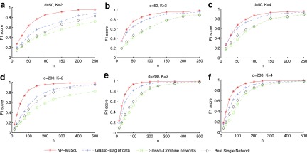
F1 score for predicting edges in simulated data, as n is varied, for (a) k = 2, (b) k = 3, and (c) k = 4 data sources for d = 50 dimensions, and for (d) k = 2, (e) k = 3, and (f) k = 4 data sources for d = 200 dimensions. The standard deviation in the results is small and almost constant across the different experiments; it ranges from (0.01-0.03), and is hence not displayed on the plot.

3.2. Effect of varying size of data sources

In the previous experiment, we assumed that each data source has an equal amount of data, that is, n_i is the same for each data source i. Next, we vary the amount of data available for different data sources and study the effects of the same on our results. For d = 200 dimensional data, we again generate simulated data for three data sources, with a total of 300 data samples across all three sources. Data source 1 has Gaussian data (identity transformed) with 100 i.i.d. data samples, data source 2 has CDF-transformed data with m samples, and data source 3 has power-transformed data with (200−m) samples. We vary m to study the effects of data sources having different amounts of data. Figure 3 shows that even when the three data sources are of different sizes, NP-MuScL performs significantly better than the other algorithms. When the amount of data in data source 2 is very small, a network learned from this data source alone has poor predictive performance, and the “Glasso-combine networks” method performs poorly since it incorporates this low-precision network in its predictions. “Glasso-bag of data” also drops its performance as m reduces, since this results in increasing importance to be placed on predictions from data source 3, which now has more data and hence a higher weight .

FIG. 3.

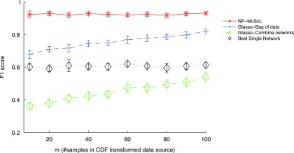
F1 score as the amount of data(m) in the data source with CDF transformation is varied. The total amount of data is kept constant by using (200 - m) samples in the data source with power transformation. The data source with an identity transformation has 100 fixed samples in all experiments.

3.3. Yeast data

In this experiment, we look at two different yeast microarray data sets and make joint predictions via NP-MuScL. Data source 1 is a set of 18 expression profiles from Cho et al. (1998), where each expression corresponds to a different stage in the cell cycle of the yeast. Data source 2 is a set of 300 expression profiles from Hughes et al. (2000), where each expression corresponds to a different knockout mutant of the yeast. Both datasets are processed using standard microarray processing algorithms (Hibbs et al., 2007).

We use a list of known interactions from BioGrid (Stark et al., 2011) to test how well the different algorithms predict the known edges. Note that since the known gene interactions are an incomplete set, predicted gene interactions may be interactions that have not yet been observed, and thus, have not been added to the BioGrid data base. Hence, measuring recall is no longer appropriate, and we report the improvement in accuracy over the random prediction of edges, as suggested by Liben-Nowell and Kleinberg (2003).

The total data is more than 6120 genes; we sample 1000 genes at a time and run the algorithms. Results are reported for 10 random subsamples of genes. Figure 4 shows the improvement over random prediction for edges predicted by each method. Because of the amount of data available, the knockout mutant expression profiles capture more information (and hence more known edges) than the time-series expression. Surprisingly, both methods of combining information without taking non-Gaussianity into account perform worse than using only data source 2. NP-MuScL is the only method where using both datasets increases the number of correctly predicted edges. The same results were found to hold true when the network is predicted over the entire set of 6120 genes—NP-MuScL did significantly better than all other methods, and both glasso-bag of data and glasso-OR did worse than using only dataset 2.

FIG. 4.

Performance of different methods of predicting edges in the yeast network. Only NP-MuScL is able to jointly use the two data sources to obtain better performance than using a single data source alone.

To test the effect of varying tuning parameter λ, Figure 5 plots the number of known edges predicted by each method versus the total number of edges predicted, as λ is varied. For very large values of λ when few edges are predicted, NP-MuScL and “glasso-bag of data” perform equally well, however, as the amount of predictions increase, NP-MuScL outperforms other methods significantly.

FIG. 5.

The effects of varying tuning parameters on different methods. For a fixed number of predicted edges, the NP-MuScL method predicts more known edges than the other methods.

Figure 6 shows the transformations learned for the two datasets by NP-MuScL for four random genes. A straight line corresponds to Gaussian data, and nonlinearities are clearly detected by the NP-MuScL algorithm. The transformations also seem to be damping extremely large values observed in the features.

FIG. 6.

Examples of the transformations made for data in source 1 (red) and source 2 (blue) for different features.

3.4. Drosophila embryonic data

We study three datasets of Drosophila embryonic gene expression for 146 genes (Tomancak et al., 2002). The first dataset measures spatial gene expression in embryonic stages 9–10 of Drosophila development via in situ hybridization (ISH) images (4.3 to 5.3 hours after fertilization), when germ band elongation of the embryo is observed. The second dataset also studies ISH images measuring spatial gene expression in stages 13–16 of embryonic development (9.3 to 15 hours after fertilization), when segmentation has already been established. The last dataset is of microarray expression at 12 time points spaced evenly in embryonic development.

The ISH images were processed to extract 311 data points for each dataset, as described in Puniyani and Xing (2012). The microarray data was processed using standard microarray processing algorithms. Since the number of data points extracted from the ISH data is dependent on the image processing algorithm used, using weights proportional to the number of data points is no longer suitable. We expect the microarray data to be as informative as the ISH data, hence we use w_i = 0.25 for each of the two ISH data sources and w_i = 0.5 for the microarray data. The results in Table 1 show that NP-MuScL outperforms using the data separately, as well as glasso-bag of data and glasso-combine networks (m = 1, called glasso-OR).

Table 1.

Improvement in Prediction over Random Guessing for Predicting Gene Interactions Using Drosophila embryonic Data

NP-MuScL	Glasso-bag of data	Glasso OR	ISH 13–16	ISH 9–10	Microarray
7.29	4.88	4.06	5.98	2.35	3.66

The bold value represents the best performance in all methods. NP-MuScL is our algorithm, OR is the OR operator (eg, OR, AND, etc.), and ISH is in situ hybridization.

We visualized the differences in edge prediction between the NP-MuScL network and the networks predicted by analyzing only one single data source at a time. The orange ellipse in Figure 7a highlights gene interactions predicted by NP-MuScL by analyzing all three data sources, which were not predicted by any single data source. Figure 7b highlights interactions predicted by microarray data that were not predicted either by the ISH data or the NP-MuScL network. The 9–10 ISH network is similar to the 13–16 ISH network, and hence, is not shown. A detailed analysis of the specific differences in the gene interactions predicted by the different methods is ongoing.

FIG. 7.

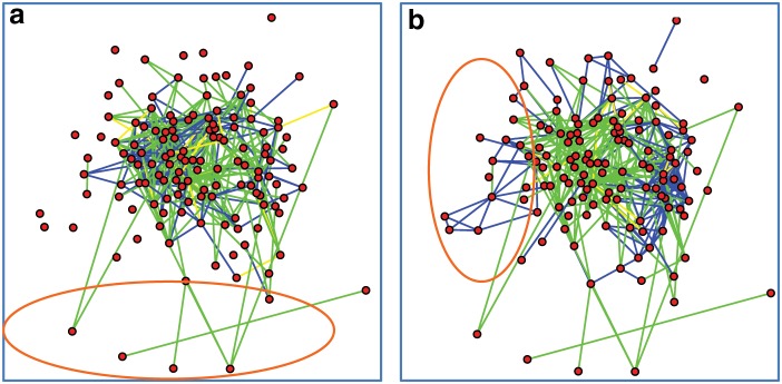
The differences between the NP-MuScL network and (a) the 13–16 ISH network alone and (b) the microarray network alone. Green edges are only predicted in the NP-MuScL network. Blue edges are only present in the (a) 13–16 ISH network and (b) the microarray network.

4. Conclusions

We proposed NP-MuScL, an algorithm that predicts gene interaction networks in a global, unsupervised fashion by jointly analyzing multiple data sources to capture the conditional independencies observed in the data. NP-MuScL models each data source as a nonparametric Gaussian copula, with all data sources having different mean and transformation functions but sharing the covariance matrix across the underlying copulas. The network can then be efficiently estimated in a two-step process of transforming each data source into Gaussian and then estimating the inverse covariance matrix of the Gaussian using all data sources jointly. We found that NP-MuScL significantly outperforms baseline methods in synthetic data as well as two experiments predicting a gene interaction network from two yeast microarray datasets and three Drosophila ISH images and microarray datasets.

One limitation of NP-MuScL is that the weights giving the importance of each data source must be assigned by the user. While a good estimate of the weights may be obtained if all data sources are truly drawn i.i.d. from their nonparanormal distributions, and have similar noise levels, in practice, some data sources may be known to be noisier than others, or known not to be i.i.d. (e.g., microarray experiments over time are not truly independent draws from the distribution). The question of automatically learning the weights from data remains an open challenge.

Acknowledgments

This research was made possible by National Institutes of Health grant (1R01GM093156) and a National Science Foundation career award (DBI 0546594) to E.P.X.

Disclosure Statement

All authors state that no competing financial interests exist.

References

- Ahmed A. Xing E.P. Tesla: Recovering time-varying networks of dependencies in social and biological studies. Proc. Natl. Acad. Sci. 2009;106:11878–11883. doi: 10.1073/pnas.0901910106. [DOI] [PMC free article] [PubMed] [Google Scholar]
- Balakrishnan S. Puniyani K. Lafferty J. Sparse additive functional and kernel cca. ICML.2012. [Google Scholar]
- Banerjee O. Ghaoui L.E. d'Aspremont A. Natsoulis G. Convex optimization techniques for fitting sparse Gaussian graphical models. ICML.2006. [Google Scholar]
- Basso K. Magolin A. Califano A. Reverse engineering of regulatory networks in human b cells. Nature Genetics. 2005;37:382–390. doi: 10.1038/ng1532. [DOI] [PubMed] [Google Scholar]
- Ben-Hur A. Noble W.S. Kernel methods for predicting protein–protein interactions. ISMB; 2005. pp. i38–i46. [DOI] [PubMed] [Google Scholar]
- Carro M.S. Califano A. Iavarone A. The transcriptional network for mesenchymal transformation of brain tumours. Nature. 2010;463:318–325. doi: 10.1038/nature08712. [DOI] [PMC free article] [PubMed] [Google Scholar]
- Cho R. Campbell M. Winzeler E. Davis R. A genome-wide transcriptional analysis of the mitotic cell cycle. Mol. Cell. 1998;2:65–73. doi: 10.1016/s1097-2765(00)80114-8. [DOI] [PubMed] [Google Scholar]
- Danaher P. Wang P. Witten D.M. The joint graphical lasso for inverse covariance estimation across multiple classes. J. R. Stat. Soc. Series B Stat. Methodol. 2013 doi: 10.1111/rssb.12033. [Epub ahead of print] [DOI] [PMC free article] [PubMed] [Google Scholar]
- Friedman J. Hastie T. Tibshirani R. Sparse inverse covariance estimation with the graphical lasso. Biostatistics. 2008;9:432–441. doi: 10.1093/biostatistics/kxm045. [DOI] [PMC free article] [PubMed] [Google Scholar]
- Goutte C. Gaussier E. A Probabilistic Interpretation of Precision, Recall and F-Score, with Implication for Evaluation, 345–359. Springer Berlin / Heidelberg. In: Losada D.E., editor; Fernández-Luna J.M., editor. Advances in Information Retrieval. Springer; Berlin/Heidelberg: 2005. [Google Scholar]
- Hibbs M. Hess D. Myers C. Troyanskaya O. Exploring the functional landscape of gene expression: directed search of large microarray compendia. Bioinformatics. 2007;23:2692–2699. doi: 10.1093/bioinformatics/btm403. [DOI] [PubMed] [Google Scholar]
- Honorio J. Samaras D. Multi-task learning of Gaussian graphical models. ICML.2011. [Google Scholar]
- Hughes T. Marton M. Jones A., et al. Functional discovery via a compendium of expression profiles. Cell. 2000:102. doi: 10.1016/s0092-8674(00)00015-5. [DOI] [PubMed] [Google Scholar]
- Katenka N. Kolaczyk E.D. Inference and characterization of multi-attribute networks with application to computational biology. Arxiv. 2012 1109.3160. [Google Scholar]
- Kolar M. Liu H. Xing E. Markov network estimation from multi-attribute data. 30th International Conference on Machine Learning; 2013. [PMC free article] [PubMed] [Google Scholar]
- Liben-Nowell D. Kleinberg J. The link prediction problem for social networks. CIKM.2003. [Google Scholar]
- Liu H. Lafferty J. Wasserman L. The nonparanormal: Semiparametric estimation of high dimensional undirected graphs. Journal of Machine Learning Research. 2009;10:2295–2328. [PMC free article] [PubMed] [Google Scholar]
- Meinshausen N. Bühlmann P. High-dimensional graphs and variable selection with the lasso. Annals of Statistics 2006 [Google Scholar]
- Morrissey E.R. Juárez M.A. Denby K.J. Burroughs N.J. On reverse engineering of gene interaction networks using time course data with repeated measurements. Bioinformatics. 2010;26:2305–2312. doi: 10.1093/bioinformatics/btq421. [DOI] [PubMed] [Google Scholar]
- Puniyani K. Xing E.P. Inferring gene interaction networks from Ish images via kernelized graphical models. 13th ECCV.2012. [Google Scholar]
- Ravikumar P. Liu H. Lafferty J. Wasserman L. Spam: Sparse additive models. NIPS.2007. [Google Scholar]
- Rothman A.J. Bickel P.J. Levina E. Zhu J. Sparse permutation invariant covariance estimation. Electronic Journal of Statistics. 2008;2:494–515. [Google Scholar]
- Segal E. Koller D. Friedman N. Module networks: identifying regulatory modules and their condition-specific regulators from gene expression data. Nature Genetics. 2003;34:166–176. doi: 10.1038/ng1165. [DOI] [PubMed] [Google Scholar]
- Stark C. Breitkreutz B. Chatr-Aryamontri A., et al. The biogrid interaction database: 2011 update. Nucleic Acids Res. 2011;39:698–704. doi: 10.1093/nar/gkq1116. [DOI] [PMC free article] [PubMed] [Google Scholar]
- Tibshirani R. Regression shrinkage and selection via the lasso. J. R. Statist. Soc. B. 1996;58:267–288. [Google Scholar]
- Tomancak P. Beaton A. Weiszmann R., et al. Systematic determination of patterns of gene expression during drosophila embryogenesis. Genome Biol. 2002;3:14. doi: 10.1186/gb-2002-3-12-research0088. [DOI] [PMC free article] [PubMed] [Google Scholar]
- Wang K. Saito M. Califano A. Genome-wide identification of post-translational modulators of transcription factor activity in human b-cells. Nature Biotechnology. 2009;27:829–839. doi: 10.1038/nbt.1563. [DOI] [PMC free article] [PubMed] [Google Scholar]
- Wang Y. Joshi T. Zhang X.-S., et al. Inferring gene regulatory networks from multiple microarray datasets. Bioinformatics. 2006;22:2413–2420. doi: 10.1093/bioinformatics/btl396. [DOI] [PubMed] [Google Scholar]
- Xu Q. Hu D.H. Yang Q. Xue H. Simpletrppi: A simple method for transferring knowledge between interaction networks for ppi prediction. Bioinformatics and Biomedicine Workshops.2012. [Google Scholar]