Considering Unknown Unknowns: Reconstruction of Nonconfoundable Causal Relations in Biological Networks

Abstract

Our current understanding of cellular networks is rather incomplete. We over look important but so far unknown genes and mechanisms in the pathways. Moreover, we often only have a partial account of the molecular interactions and modifications of the known players. When analyzing the cell, we look through narrow windows leaving potentially important events in blind spots. Network reconstruction is naturally confined to what we have observed. Little is known on how the incompleteness of our observations confounds our interpretation of the available data. Here we ask which features of a network can be confounded by incomplete observations and which cannot. In the context of nested effects models, we show that in the presence of missing observations or hidden factors a reliable reconstruction of the full network is not feasible. Nevertheless, we can show that certain characteristics of signaling networks like the existence of cross-talk between certain branches of the network can be inferred in a nonconfoundable way. We derive a test for inferring such nonconfoundable characteristics of signaling networks. Next, we introduce a new data structure to represent partially reconstructed signaling networks. Finally, we evaluate our method both on simulated data and in the context of a study on early stem cell differentiation in mice.

1. Introduction

In February 2002, Donald Rumsfeld, then the U.S. Secretary of Defense, stated at a Defense Department briefing that: “There are known knowns. There are things we know that we know. There are known unknowns. That is to say, there are things that we now know we don't know. But there are also unknown unknowns. There are things we do not know we don't know” (Rumsfeld, 2002). The concept of unknown unknowns is eminent to many fields of research. In the context of biological networks, known knowns make up our literature knowledge on physical and functional interactions of signaling molecules. Known unknowns might be what our current research projects are about, but unknown unknowns are those cellular mechanisms that we do not even anticipate today. They can be best appreciated in a historic perspective: Today, the role of many micro RNAs and epigenetic modifications of chromatin structure are known known mechanisms in many pathways. For other instances, they are still in the realm of known unknowns. But going back 15 years in history, they were unknown unknowns. Models of signaling pathways did not include them, and the vast majority of molecular biologists did not anticipate the important role they play.

Once unknown unknowns become known, two different scenarios can occur: (i) The new observations can add to our understanding of a network or (ii) they can fundamentally change our perspective of the networks. In scenario (i), the network becomes more nodes and edges, but the already existing parts of the network do not change. In scenario (ii), we learn that our old working hypothesis of the network was confounded by the mechanisms of which we were not aware. The hidden effects of unknown unknown players made the interplay of the known players appear different than they really are.

This raises the question, what of our current understanding of biological networks can be confounded by hidden mechanisms and what cannot. We believe the question can only be addressed meaningfully in the context of a formal statistical network reconstruction framework, like Bayesian networks (Friedman et al., 2000), Gaussian graphical networks (Schfer and Strimmer, 2005), Boolean networks (Saez-Rodriguez et al., 2009), or nested effects models (Markowetz et al., 2005).

In these frameworks, unknown unknowns are a set of hidden nodes. Together with the observed nodes they form a directed large biological network. The edges of the network encode causal relations. This means that if there is a directed edge from A to B, then perturbing A leads to changes in B. We call this large network the ground truth network (GTN). In practice, it is almost always unknown. Observed and modeled is only a subset of the GTN nodes, resulting in a “current state-of-the-art network” (CSAN). This network only connects observed nodes. Importantly, in the GTN the hidden nodes can affect the observed nodes. A CSAN is reconstructed correctly if it is identical to the subnetwork that the observed nodes form in the GTN. However, such a subnetwork does not need to exist (Elidan et al., 2002). Clearly, in such a case every network built exclusively from observed nodes is incorrect.

The problem of hidden nodes in network analysis has been recognized for a long time, for example, in causal inference theory (Pearl, 2000). In the context of Bayesian network reconstruction, the structural expectation maximization (EM) algorithm can be used (McLachlan and Krishnan, 1997) to account for some missing observations. Moreover, the concept of structural signatures facilitates the detection and approximate location of a hidden variable in a network (Elidan et al., 2002). However, latent variable approaches are only practical if the number of hidden nodes is small, an assumption that is questionable, and it is often violated in the domain of molecular biology.

The reconstruction of a correct subnetwork from very incomplete observations might be too ambitious. Alternatively, one can strive for deriving features of a network that are correct, no matter what is going on outside of the observation window. Colombo et al. (2011) introduced the concept of partial ancestral graphs (PAG), extending the work in Richardson and Spirtes (2002). A PAG describes the common causal features of all directed acyclic graphs (DAGs) that cannot be reliably distinguished if one accounts for possible effects of hidden nodes. The PAG is not a fully resolved network. Its information content lies in the features of the networks it excludes, since this exclusion is guaranteed not to be an artifact caused by hidden nodes. The inference is not confoundable. Colombo et al. (2011) describe a computationally efficient algorithm that allows for the asymptotically consistent estimation of sparse high-dimensional PAGs. A charming feature of the method is that it works exclusively using observational data. Practical drawbacks are the limited biological interpretability of general Bayesian networks learned on gene expression data and missing to exploiting functional information revealed in cell perturbation experiments. In fact, applications to molecular biology have not been reported to date.

Here we consider the concept of a partial but not confoundable network reconstruction in the context of nested effects models (NEMs) (Markowetz et al., 2005). NEMs differ from the more general networks designed by Colombo et al. in two ways: (i) They are learned from interventional data, and (ii) all edges except for those involving leaf nodes encode deterministic information flow, for example, local transition probabilities are zero or one. NEMs assume that the cellular information flow is deterministic; stochasticity only comes in via noisy observations (Zeller et al., 2009). These features make nonconfoundable network inference simpler and allow for straightforward applications in systems biology.

This article is organized as follows. In the context of nested effects models, we show that in the presence of unknown unknowns, network reconstruction can be flawed. We introduce a simple edge-by-edge partial network reconstruction algorithm called nonconfoundable network analysis (No-CONAN) to derive nonconfoundable network properties. In analogy to PAGs, we define a data structure that encodes the partially resolved networks (pNEM, for partial nested effects model). On simulated data, we demonstrate the performance of our algorithm, and in a first application to embryonic stem cell differentiation in mice, we demonstrate that taking unknown unknowns into account changes our account of real biological networks.

2. Methods

2.1. Nested effects models

For self-containedness, we briefly review nested effects models as introduced in Markowetz et al. (2005). NEMs learn upstream/downstream relations in nontranscriptional signaling pathways from the nesting of transcriptional downstream effects when perturbing the signaling genes. In a nutshell, NEMs infer that gene A operates upstream of gene B in a pathway if the downstream effects resulting from silencing gene B are a noisy subset of those resulting from silencing gene A. Following Markowetz et al. (2005), we call the perturbed genes in the signaling pathway S-genes and the genes that show expression changes in response to perturbation E-genes.

An NEM is a directed and possibly cyclic network that connects the S-genes representing the flow of information in the underlying signaling pathway. E-genes can be linked to single S-genes forming leaf nodes of the network. The directed edges linking E-genes to S-genes can be estimated together with the S-gene network (Tresch and Markowetz, 2008), or they can be taken by Bayesian maximum a posteriori approach (Niederberger et al., 2012), or they can be treated as nuisance parameters that are integrated out (Markowetz et al., 2005, 2007; Anchang et al., 2009).

The underlying data consists of gene expression profiles of gene silencing assays and corresponding controls. Typically, a pathway is stimulated both in cells where it is intact (controls) and in cells where it is partially disrupted by silencing one of its S-genes. If the silencing of an S-gene blocks the flow of information from the pathway initiating receptors to the E-gene, the E-gene no longer changes expression in response to stimulation. In the language of nested effects models the E-gene shows a silencing effect with respect to the S-gene, and the crucial assumption is that E-genes must attach to at most one S-gene. In each experiment, one S-gene is silenced by RNAi, and silencing effects on thousands of E-genes are measured. The expression data D_ij is assumed to be discretized to 0 and 1, with a 1 indicating that a silencing effect of S_j was observed on E_i. Signal propagation within the pathways is assumed to be deterministic, hence the silencing of S_j is expected to produce silencing effects in all E-genes downstream of S_j. Consequently, every network topology is associated with an expected data pattern across all silencing assays—the silencing scheme (Markowetz et al., 2005). If the network is acyclic, the silencing scheme defines a partial order relation on the S-genes reflecting the expected nesting of downstream effects. Noise comes into play at the level of observations. NEMs allow for both false positive and false negative observations, accounting for them by fixed rates α and β in the likelihood. Hence, NEMs aim to detect a noisy subset relation in the observations D_ij and represent it as a directed network, where the directed edges can be interpreted as upstream/downstream relations of genes in the pathway. Clearly if gene A is upstream of gene B, and B is upstream of gene C, then A must be upstream of C as well. This is reflected in the likelihood equivalence of all networks that have the same transitive closure. In other words, NEMs are a degenerate type of Bayesian network in which all non-leaf nodes are not observable and all edges between S-genes are associated with 0/1 local probabilities (Zeller et al., 2009). While the first property makes network reconstruction hard, the second is a simplification that renders network reconstruction practical again.

Several extensions of NEMs exist, including networks that distinguish activation and repression (Vaske et al., 2009), likelihoods allowing continuous silencing data (Tresch and Markowetz, 2008; Fröhlich et al., 2008b), dynamic models (Anchang et al., 2009; Fröhlich et al., 2011), and models including direct observations of S-gene activation (Bender et al., 2010). The methodology is implemented in a bioconductor package nem and cran package nessy (Fröhlich et al., 2008a). A comprehensive review and evaluation can be found in Fröhlich et al. (2009).

2.2. Hidden nodes compromise NEM-based network reconstruction

For general Bayesian networks, it is well known that hidden nodes can confound the reconstruction of networks (Colombo et al., 2011; Koller and Friedman, 2009). Here we show that this problem still exists for the more specialized NEM. We generated data for networks that include both observed and unobserved nodes and reconstruct the subnetwork of observed nodes: We generated 100 random networks of four nodes and extended them by n = 0,4,8,16 additional hidden nodes. Artificial silencing data was generated for the extended networks as described previously (Markowetz et al., 2005). Only the data for the four observable nodes was used to reconstruct four node networks. These were compared to the corresponding subnetworks of the larger networks. The extended networks represent the ground truth signaling pathway while the four node subnetworks represent the small window through which we observe it. Figure 1 shows positive predicted values of network reconstruction (y-axis) for different noise levels (x-axis). The red line corresponds to network reconstruction without hidden nodes, while the green, blue, and purple lines refer to 4, 8, and 12 additional hidden nodes respectively. We observe a marked decrease in network reconstruction performance when hidden nodes can confound the flow of information of the observed nodes.

FIG. 1.

In simulations, hidden nodes compromise network reconstruction: Shown is the accuracy of standard nested effects model (NEM)-based network reconstructions if hidden nodes are present. The x-axis shows the degree of noise used in the stimulations. The y-axis shows the positive predictive value of reconstructed edges of the subnetwork of observed nodes. The different lines correspond to different numbers of hidden confounders (red 0, green 4, blue 8, purple 12).

2.3. Alien silencing patterns are the clue to a non-confoundable network analysis

We analyze all pairs of S-genes S₁ and S₂ separately using only the data from silencing S₁ and S₂. Since our analysis will be nonconfoundble by genes outside of the observation window, it will also not be affected by the remaining S-genes that we Purposely did not take into account.

For a pair of genes S₁ and S₂, we distinguish five possible upstream/downstream relations summarized in Figure 2A. (R1) S₁ is upstream of S₂, (R2) S₁ is downstream of S₂, (R3) S₁ and S₂ lie in a feedback loop in which case they are both up and downstream from each other as indicated by the double arrow, (R4) S₁ and S₂ lie in independent modules of the network and do not interact with each other at all, and (R5) S₁ and S₂ are in different branches of a signaling network but jointly regulate at least one possibly hidden S-gene H. The five relations are encoded by the different edge types:

(1)

FIG. 2.

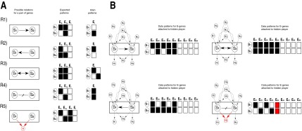
Pairwise upstream/downstream relations and their alien patterns: (A) Shown are the five possible possible relations together with their expected silencing patterns and their alien patterns. (B) Hidden nodes are introduced in all possible configurations, and the expected patterns of E-genes attached to the hidden nodes are shown. In (R4) the hidden node marked in red produces the alien pattern of (R4). Note that this constellation leads to the constellation in (R5).

With only two S-genes, an E-gene can show four different silencing patterns: It responds to both perturbations (1,1), only to one of them (1,0) and (0,1), or to none (0,0). Each upstream/downstream relation induces an expected subset of these four patterns. For example, in relation (R1) an E-gene can be unconnected to both S₁ and S₂ in which case it does not show a silencing effect neither when silencing S₁ nor when silencing S₂, yielding the expected pattern (0,0). It can be attached to S₁ in which case it is expected to show an effect when silencing S₁ but not when silencing the downstream gene S₂, yielding the expected pattern (1,0). And last, it can be linked to S₂ and show silencing effects both when silencing S₁ and S₂, yielding the pattern (1,1). Figure 2A gives the set of expected silencing patterns for all five upstream/downstream relations. Note that only relation R5 can produce all four possible silencing patterns. For the remaining relations, at least one pattern is not expected. We call these unexpected patterns alien patterns.

We next investigated the possible influence of hidden nodes on the sets of expected and alien patterns (Fig. 2B). There are nine possible positions of a hidden confounder. The silencing patterns associated with these positions are shown in Figure 2B. The most important observation is that any position of hidden confounders in the network does not change the sets of expected and alien silencing patterns (Fig. 2B). Note that in (R4) the hidden node marked in red produces the alien pattern of (R4). However, we have accounted for this problem by distinguishing the two relations (R4) and (R5) from the beginning. The conclusion that no alien patterns can occur through confounding facilitates our nonconfoundable analysis: If the observation of an alien pattern cannot be through confounding effects it must be due to noise in the observation. Note that the assumption of deterministic signal propagation is crucial here. In relation (R1) we assume that a perturbation of S₁ is deterministically propagated to S₂, which rules out the silencing pattern (0,1).

2.4. The accumulation of alien patterns is evidence against respective upstream/downstream relations

For a pair of S-genes, we can systematically consider all five upstream/downstream relations and see whether they conform to the observed data. Each of the relations (R1)–(R4) has at least one alien pattern. Every observation of an E-gene that displays this alien pattern is evidence against the respective relation. Few alien patterns can occur due to observation noise, but a large number of alien patterns is unlikely. We will set up a test to detect significantly high occurrences of alien patterns.

Binary NEMs (Markowetz et al., 2005) model observation noise by a false positive rate α, the probability that an observed effect is a noise artifact and a false negative rate β, and the probability that we miss a true silencing effect. Further, the occurrence of observation errors is assumed to be independent across E-genes. We can derive limits for the probability that a certain number k of alien patterns occur given a relation . This derives from the property of a binomial distribution(n, p) that its tail probability is monotonically increasing with the parameter p. A proof is provided for completeness. For given k, n, 0 ≤ k ≤ n, and , let . Define T(p;k, n) = P(x ≥ k ∣ n, p). Then we wish to show that T is monotonically increasing in p. Taking the derivative, we obtain

where the last equality can be proved by induction.

1. The equality clearly holds true for k = 0 since T(p;0, n) = 1, hence T′(p;0, n) = 0, and

for k = 0.

2. Assume now that it holds for k. For k + 1 one gets

which concludes the proof.

Consider now for example the case R = R1, then we have

(2)

where k is the observed number of alien patterns, n the total number of E-genes, and γ_R1 an upper bound for the probability of observing the alien pattern. If (R1) holds true, the alien pattern (0, 1) needs to be produced by noise from one of the three expected patterns (1,0), (1,1), and (0,0). Starting from (1,0) requires both a false positive and a false negative observation, which happens with probability γ₁ = α · β, starting from (1,1) we need one true positive and one false negative observation, which occurs with probability γ₂ = β · (1−β). Finally, generating the alien pattern (0,1) from (0,0) requires one true negative and one false positive observation and occurs with probability γ₃ = (1−α) · α. Setting γ_R1 = max(γ₁, γ₂, γ₃) yields the bound (2). Similarly we obtain:

(3)

for all . Here γ_R is a bound for the probability of observing the alien pattern of R. If some of the above probabilities become sufficiently small, we gather evidence against the respective relations. We exclude a relation R if and only if

(4)

where κ is a calibration parameter that is set to 0.05 in all applications below. Note that R5 cannot be rejected since it does not have an alien pattern.

2.5. Partial network reconstruction

If R5 is correct and we can reject relations R1–R4, leaving only relation R5 as compatible with the data, we have fully resolved the relation of S₁ and S₂. In cases where R5 is incorrect, the best we can achieve is that all but one relation from R1–R4 is rejected, leaving us with one edge type, and the always existing possibility that R5 is true. However, this does not need to be the case. It is possible that we cannot reject several relations, leaving us with higher uncertainties on the true structure of the signaling network. We do not further resolve the network but confine ourselves to describing what we know and what we don't know. To do this, we introduce the new data structure of a partial nested effects model (pNEM). A pNEM is a graph connecting all S-genes, however, using a variety of different edge types. Each edge type is describing a set of relations that could not be rejected. This language of edge types is summarized in Figure 3. For example, if we exclude all relations except (R5), there is no edge between S₁ and S₂. If we reject all relations except R3, R4, and R5, we draw a red double-sided edge, and so on. Sixteen different edge types are needed to encode our partial network knowledge. In the next section, we show an example of a pNEM.

FIG. 3.

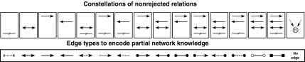
The partial nested effects model (pNEM) code: The top row of boxes shows combinations of relations, and the bottom boxes show the corresponding edge types we use to encode that none of the edges in the set could be excluded by nonconfoundable network analysis (No-CONAN).

Equation (4) has the form of a statistical test. When choosing κ sufficiently small, we bound the probability of excluding a correct relation. The null hypothesis is that the tested relation is correct and that all observed alien patterns are due to noise alone. However, a small κ also leads to poorly resolved networks with only few excluded relations. This raises the issue of the power of the test. An edge between two S-genes is well resolved if the true relation generates many E-genes with silencing patterns that are alien to many alternative relations. For example, if the relation S₁ → S₂ holds true, every E-gene that is attached to S₁ and produces the expected pattern (1,0) produces evidence against the competing relations S₁ ← S₂ and S₁ ↔ S₂, since (1,0) is alien to both these relations, but not against the relation S₁ · · S₂, since (1,0) is not alien to it. However, E-genes attached to S₂ with the expected pattern (1,1) produce evidence against S₁ · · S₂. If we have enough E-genes of both types, we will be able to reject all relations except the correct one and the not-rejectable relation R5. Inspecting Figure 2 points to a problem with edges that are of the type S₁ ↔ S₂, since in this constellation only the patterns (1,1) and (0,0) are produced but none of the alien patterns of the two directed relations R1 and R2. Since NEMs operate on transitively closed networks, the relation S₁ ↔ S₂ is indicative of genes involved in a feedback loop. In other words, our method is not capable of reliably detecting feedback loops; a noncircular constellation often can not be ruled out. Nevertheless, our method is valid also for biological networks with feedback loops. It does not produce spurious results in this case, but reports that it cannot resolve the loop reliably. If, in contrast, the true network is not cyclic, our method has the potential to exclude a loop reliably.

3. Simulation Experiments

We test the performance of No-CONAN in the context of simulation experiments using artificial data. In such simulations, the true state of the network is known, unlike in biological scenarios. Moreover, the artificial data fully conforms to all assumptions of NEMs, which is certainly not the case for real biological data.

3.1. Example

We start with an example to illustrate how No-CONAN works. Consider the GTN in Figure 4. Note that it has only one hidden node, but this node is in a central position of the network. We attach a total of 350 E-genes uniformly to the S-genes and generate artificial data using moderate noise levels of 0.15 for both false negative and false positive observations as described previously (Markowetz et al., 2005). Then, using only data for the observable nodes, we reconstruct the network using triplet search in a standard NEM approach (Markowetz et al., 2007) and using No-CONAN. Figure 4 compares the NEM to the pNEM. The NEM incorrectly predicts a feedback loop–like structure. The pNEM in contrast did not do this. It actually resolved the relation between S₅ and S₆ as R5, thus predicting the existence of the hidden node at that position. Also, all other predicted relations are correct, with the exception of S₆ and S₃, where the pNEM is undecided whether a directed relation exists (incorrect) or not (correct).

FIG. 4.

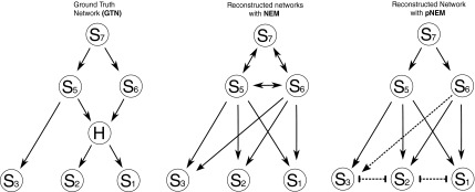
Performance comparison: The left part of the figure shows a GTN that has one hidden node. We attach a total of 350 E-genes uniformly to the S-genes and generate artificial data using a moderate noise level of 0.15 for both false negative and false positive observations. The plots in the middle and on the right side of the figure show the reconstructed network using triplet search in a standard NEM approach and pNEM, respectively, only for the observable nodes. The NEM incorrectly predicts a feedback loop–like structure. In contrast, the pNEM resolved the relation between S₅ and S₆ as R5, thus predicting the existence of the hidden node at that position. Also, all other predicted relations are correct, with the exception of S₆ and S₃, where the pNEM is undecided whether a directed relation exists (incorrect) or not (correct).

3.2. Evaluations

We generate 100 random networks of size eight and generate data for these networks using noise levels varying between 0.005 (very low) and 0.32 (very high). We attach a total of 100 E-genes uniformly to the S-genes of the network and add another 900 E-genes that are unrelated to the networks. These have an expected silencing pattern of (0,0) but display occasional silencing effects due to noise. We then run No-CONAN on every pair of nodes in each of 100 networks and reject all relations possible using κ = 0.05. The results are organized according to the true underlying relations in Figure 5A. Each of the five plots corresponds to one true relation. The x-axis shows the different noise levels while the y-axis shows the relative frequency of rejecting the different relations, which are marked by different colors. For example, the left-most plot corresponds to all situations in which the true relation between nodes is S₁- → S₂. Rejection rates for this relation are marked in blue, and we can see that the relation does not get falsely rejected even for very high noise levels. In contrast, the three competing relations marked in red, purple, and green are virtually always rejected except for very high noise levels, and even for maximal noise we reject them in about half the cases. We do similarly well for the next two relations. If the true relation is the feedback loop S₁ ↔ S₂, we still get hardly any false positive rejections but lose almost all power in rejecting the two directed relations. As described in the previous section, this is expected since a feedback loop does not produce the alien patterns of these relations.

FIG. 5.

(A) Small network simulations. Each of the five plots corresponds to one true relation. The x-axis shows the different noise levels. The y-axis shows the relative frequency of rejecting the relations (R1: blue, R2: purple, R3: green, R4: red, and R5: orange). (B) Simulations on a large network. Left: The ground truth network. Right: Performance plots that organized like in (A).

3.3. Large numbers of unrelated E-genes compromise the resolution of No-CONAN

E-genes that are not related to the modeled pathway produce the silencing pattern (0,0) for all perturbations of pathway genes. The pattern (0,0) is an expected pattern for all relations in (Fig. 2A). In noisy data some unrelated E-genes produce patterns different from (0,0), including alien patterns. With more unrelated E-genes, more alien patterns are expected due to noise, and it becomes more difficult for the true alien patterns to stand out. This compromises the power of our test. To quantify this effect, we generate 100 random networks of size eight and generate data for these networks with different numbers of unrelated E-genes. We attach a total of 100 E-genes uniformly to the S-genes of the network and add another {0, 100, 500, 1000} E-genes, which are unrelated to the networks. We run No-CONAN on every pair of nodes in each of the networks and reject relations on the level κ = 0.05. The results are organized according to the true underlying relations in Figure 6. As expected, the power of our test drops with increasing numbers of unrelated E-genes. However, even for the maximal number of 10 times unrelated to related genes, we still reject a considerable number of relations and hence still learn features of the network in a nonconfoundable way.

FIG. 6.

The number of unrelated E-genes might effect the power of the testing: Rows correspond to the number of unrelated E-genes in the simulated data sets (0, 100, 500, 1000), while columns represent true relations. In each plot, the x-axis shows the different noise levels while the y-axis shows the relative frequency of rejecting the different relations, which are marked by different colors (R1: blue, R2: purple, R3: green, R4: red, and R5: orange). Results show that the number of unrelated E-genes effect the power of the test. We still have hardly any false-positive rejections but gain power in rejecting the incorrect relations by decreasing the number of E-genes with (0,0) pattern.

3.4. Evaluations on a large network

We examine the performance of No-CONAN in the context of the larger 25-node network shown in Figure 5B. Note that the network contains two feedback loops, one toward the root and another one close to a leaf. The crucial difference from the smaller networks is the ratio of S-genes inside the observation window (two in both cases) and those outside of it (6 vs. 23). In fact, this unfavorable ratio of observed versus unobserved nodes compromises the resolution of the pNEMs generated by No-CONAN. Importantly, we still hardly ever falsely reject a correct relation. However, except for very low noise levels rejection rates of incorrect relations decrease. Nevertheless, except for very high noise levels, we reject substantial fractions of relations thus partially learning the structure of the network.

4. An Application to Murine Stem Cell Development

We test No-CONAN in a study on molecular mechanisms of self-renewal in murine embryonic stem cells (ESCs). Ivanova et al. (2006) down-regulated six factors (Nanog, Oct4, Sox2, Esrrb, Tbx3, and Tcl1) that need to be jointly expressed in murine ESCs to keep the cells in a self-renewal state. In response to the interventions the cells go into differentiation, and the resulting shifts in the transcriptome were monitored in time series of expression profiles. Differentiation includes the successive destruction of the self-renewal network. This process of differentiation has been previously modeled twice using nested effect models (Anchang et al., 2009; Fröhlich et al., 2011). Both models have in common that they are dynamic nested effects models exploiting the temporal information of the time series but differ in the likelihood functions used. None of them considered the possibility of unobserved factors.

In the NEM framework, Nanog, Oct4, Sox2, Esrrb, Tbx3, and Tcl1 are S-genes, whereas genes showing expression changes in response to silencing are E-genes. A silencing effect is observed if the expression of an E-gene is pushed from its level in self-renewing cells to its level in differentiated cells. We preprocess and discretize the data as described in Anchang et al. (2009). Then we run No-CONAN on the data of the last time point of all time series. Figure 7A shows the pNEM produced from No-CONAN while 7C and D are the transitive closures of the networks derived in Anchang et al. (2009) and Fröhlich et al. (2011).

FIG. 7.

Murine stem cell self-renewal network: (A) shows the partial nested effects model (pNEM) produced from No-CONAN. (B) shows prediction results from the observation that all relations except for R5 could be excluded for the respective pairs of genes. The pNEM predicts the existence of certain hidden nodes in positions marked in (B). (C) and (D) are the transitive closures of the networks derived in Anchang et al. (2009) and Fröhlich et al. (2011). Many edges of the pNEM are optimally resolved and often agree with those in the two previous models in (C) and (D).

Notably, many edges of the pNEM are optimally resolved and often agree with those in the two previous models, for example, the linear backbone of the network Nanog → Sox2 → Oct4 observed in the Anchang model (Anchang et al., 2009) could be resolved unambiguously even when taking hidden confounders into account.

In contrast, the role of the remaining genes Tcl1, Tbx3, and Esrrb could not be determined unambiguously with the available observations. For example, our pNEM proclaims that there is an interaction between Esrrb and Tbx3 but can not determine its nature. It could be a feedback loop as well as any directed edge depending on how a potential unknown gene is influencing the process. Moreover, the pNEM differs from the two NEMs in that it predicts the existence of certain hidden nodes in positions marked in Figure 7B. These predictions result from the observation that all relations except for R5 could be excluded for the respective pairs of genes. In summary, nonconfoundable analysis sustains a previous hypothesis on the role of Nanog, Sox2, and Oct4 interactions in stem cell differentiation but also points to possible ambiguities with respect to the role of Tcl1, Tbx3, and Esrrb.

5. Discussion

We introduced No-CONAN, a novel method that partially reconstructs the upstream/downstream relations of nontranscriptional signaling networks from interventional data. The method is set in the framework of nested effects models but has the additional feature that its inference cannot be confounded by hidden nodes. The key idea is the definition of alien silencing patterns that cannot be confounded by unobserved nodes. The output of No-CONAN is not a fully resolved network but a pNEM: A network of upstream/downstream relations in which for some pairs of nodes several relations remain conformable with the data. The information in a pNEM lies in the upstream/downstream relations that it excludes. A pNEM encodes what we know but also what we cannot know unless we can be sure that we have observed all nodes of a network. The uncertainties left with certain edges are the price we have to pay to ensure that our results are nonconfoundable by mechanisms outside the window of observations.

No-CONAN is reliable in that it does not produce false information by rejecting correct relations. By construction, No-CONAN has two limitations affecting its power in resolving the network. It can never reject the relation S₁ → H ← S₂, since this relation has no alien silencing patterns. Moreover, No-CONAN has very little power in resolving a true feedback loop since feedback does not produce the alien patterns of the two directed relations. Nevertheless, No-CONAN is generating new nonconfoundable insights into network structures by rejecting many, though not all, incorrect relations.

Partial network reconstruction is a relatively new concept in network analysis. It can be seen as a safeguard against possibly severe confounding effects caused by unobserved mechanisms. Clearly, such a nonconfoundable analysis is only valid within the formal context of a network model. In this article, we used the framework of nested effects models. The assumptions of nested effects models might be incorrect in certain applications as is true for every modeling framework. We believe that no formal analysis can safeguard against this. However, the concept of unknown mechanisms can be represented in many formal frameworks, and simulations can mimic our partial observation of a true underlying network. Here we represented all the unknown unknowns of biology as unobserved nodes of nested effects models and strived for extracting as much information on the full nested effects models from the incomplete data we obtained by looking through a narrow window.

Donald Rumsfeld continued his speech by saying, “If I know the answer I'll tell you the answer, and if I don't, I'll just respond, cleverly.” (Rumsfeld, 2002) We do not know whether a pNEM is a “clever” response, but it aims to be a realistic and an honest one. The partial network aims to encode what we know that we know, but it also encodes what we cannot know for certain, unless we are absolutely sure that we have a complete account of all biological mechanisms affecting cell signaling.

Acknowledgments

This work was supported by BMBF grants (EraSys:0315714B) and the Bavarian Genome Network BayGene. We thank Achim Tresch for fruitful discussions, and Florian Markowetz, Christian Hundsrucker, Julia C. Engelmann, and Claudio Lottaz for carefully proofreading the manuscript.

References

- Anchang B. Sadeh M.J. Jacob J., et al. Modeling the temporal interplay of molecular signaling and gene expression by using dynamic nested effects models. Proc. Natl. Acad. Sci. USA. 2009;106:6447–6452. doi: 10.1073/pnas.0809822106. [DOI] [PMC free article] [PubMed] [Google Scholar]
- Bender C. Henjes F. Fröhlich H., et al. Dynamic deterministic effects propagation networks: learning signalling pathways from longitudinal protein array data. Bioinformatics. 2010;26:i596–i602. doi: 10.1093/bioinformatics/btq385. [DOI] [PMC free article] [PubMed] [Google Scholar]
- Colombo D. Maathuis M. Kalisch M., et al. Learning high-dimensional directed acyclic graphs with latent and selection variables. Arxiv preprint. 2011 arXiv:1104.5617. [Google Scholar]
- Elidan G. Ninio M. Friedman N., et al. Data perturbation for escaping local maxima in learning. AAAI/IAAI. 2002:132–139. [Google Scholar]
- Friedman N. Linial M. Nachman I., et al. Using Bayesian networks to analyze expression data. J. Comput. Biol. 2000;7:601–620. doi: 10.1089/106652700750050961. [DOI] [PubMed] [Google Scholar]
- Fröhlich H. Beißbarth T. Tresch A., et al. Analyzing gene perturbation screens with nested effects models in r and bioconductor. Bioinformatics. 2008a;24:2549–2550. doi: 10.1093/bioinformatics/btn446. [DOI] [PMC free article] [PubMed] [Google Scholar]
- Fröhlich H. Fellmann M. Sültmann H., et al. Estimating large-scale signaling networks through nested effect models with intervention effects from microarray data. Bioinformatics. 2008b;24:2650–2656. doi: 10.1093/bioinformatics/btm634. [DOI] [PMC free article] [PubMed] [Google Scholar]
- Fröhlich H. Tresch A. Beißbarth T. Nested effects models for learning signaling networks from perturbation data. Biom. J. 2009;51:304–323. doi: 10.1002/bimj.200800185. [DOI] [PubMed] [Google Scholar]
- Fröhlich H. Praveen P. Tresch A. Fast and efficient dynamic nested effects models. Bioinformatics. 2011;27:238–244. doi: 10.1093/bioinformatics/btq631. [DOI] [PubMed] [Google Scholar]
- Ivanova N. Dobrin R. Lu R., et al. Dissecting self-renewal in stem cells with RNA interference. Nature. 2006;442:533–538. doi: 10.1038/nature04915. [DOI] [PubMed] [Google Scholar]
- Koller D. Friedman N. Probabilistic graphical models: principles and techniques. The MIT Press; 2009. [Google Scholar]
- Markowetz F. Bloch J. Spang R. Non-transcriptional pathway features reconstructed from secondary effects of RNA interference. Bioinformatics. 2005;21:4026–4032. doi: 10.1093/bioinformatics/bti662. [DOI] [PubMed] [Google Scholar]
- Markowetz F. Kostka D. Troyanskaya, et al. Nested effects models for high-dimensional phenotyping screens. Bioinformatics. 2007;23:i305–i312. doi: 10.1093/bioinformatics/btm178. [DOI] [PubMed] [Google Scholar]
- McLachlan G. Krishnan T. The EM algorithm and extensions. Vol. 274. Wiley New York; 1997. [Google Scholar]
- Niederberger T. Etzold S. Lidschreiber M., et al. Mc eminem maps the interaction landscape of the mediator. PLoS Comput. Biol. 2012;8:e1002568. doi: 10.1371/journal.pcbi.1002568. [DOI] [PMC free article] [PubMed] [Google Scholar]
- Pearl J. Causality: Models, Reasoning, and Inference. Vol. 47. Cambridge University Press; Cambridge, United Kingdom: 2000. [Google Scholar]
- Richardson T. Spirtes P. Ancestral graph Markov models. The Annals of Statistics. 2002;30:962–1030. [Google Scholar]
- Rumsfeld D. DOD news briefing—Secretary Rumsfeld and Gen. Myers. U.S. Department of Defense 2002 [Google Scholar]
- Saez-Rodriguez J. Alexopoulos L.G. Epperlein J., et al. Discrete logic modelling as a means to link protein signalling networks with functional analysis of mammalian signal transduction. Mol. Syst. Biol. 2009;5:331. doi: 10.1038/msb.2009.87. [DOI] [PMC free article] [PubMed] [Google Scholar]
- Schfer J. Strimmer K. An empirical bayes approach to inferring large-scale gene association networks. Bioinformatics. 2005;21:754–764. doi: 10.1093/bioinformatics/bti062. [DOI] [PubMed] [Google Scholar]
- Tresch A. Markowetz F. Structure learning in nested effects models. Stat. Appl. Genet. Mol. Biol. 2008;7:9. doi: 10.2202/1544-6115.1332. Article. [DOI] [PubMed] [Google Scholar]
- Vaske C.J. House C. Luu T., et al. A factor graph nested effects model to identify networks from genetic perturbations. PLoS Comput. Biol. 2009;5:e1000274. doi: 10.1371/journal.pcbi.1000274. [DOI] [PMC free article] [PubMed] [Google Scholar]
- Zeller C. Fröhlich H. Tresch A. A Bayesian network view on nested effects models. EURASIP J. Bioinform. Syst. Biol. 2009:195272. doi: 10.1155/2009/195272. [DOI] [PMC free article] [PubMed] [Google Scholar]