Segmentation, Feature Extraction, and Multiclass Brain Tumor Classification

Abstract

Multiclass brain tumor classification is performed by using a diversified dataset of 428 post-contrast T1-weighted MR images from 55 patients. These images are of primary brain tumors namely astrocytoma (AS), glioblastoma multiforme (GBM), childhood tumor-medulloblastoma (MED), meningioma (MEN), secondary tumor-metastatic (MET), and normal regions (NR). Eight hundred fifty-six regions of interest (SROIs) are extracted by a content-based active contour model. Two hundred eighteen intensity and texture features are extracted from these SROIs. In this study, principal component analysis (PCA) is used for reduction of dimensionality of the feature space. These six classes are then classified by artificial neural network (ANN). Hence, this approach is named as PCA-ANN approach. Three sets of experiments have been performed. In the first experiment, classification accuracy by ANN approach is performed. In the second experiment, PCA-ANN approach with random sub-sampling has been used in which the SROIs from the same patient may get repeated during testing. It is observed that the classification accuracy has increased from 77 to 91 %. PCA-ANN has delivered high accuracy for each class: AS—90.74 %, GBM—88.46 %, MED—85 %, MEN—90.70 %, MET—96.67 %, and NR—93.78 %. In the third experiment, to remove bias and to test the robustness of the proposed system, data is partitioned in a manner such that the SROIs from the same patient are not common for training and testing sets. In this case also, the proposed system has performed well by delivering an overall accuracy of 85.23 %. The individual class accuracy for each class is: AS—86.15 %, GBM—65.1 %, MED—63.36 %, MEN—91.5 %, MET—65.21 %, and NR—93.3 %. A computer-aided diagnostic system comprising of developed methods for segmentation, feature extraction, and classification of brain tumors can be beneficial to radiologists for precise localization, diagnosis, and interpretation of brain tumors on MR images.

Introduction

The process of brain tumor classification is one of the most challenging tasks as isointense (same signal intensity as that of brain tissues) to hypointense (darker than the brain tissues) property of brain tumors, heterogeneity, and associated perilesional edema creates ambiguity in tumor classification. Generally, contrast-enhanced T1-weighetd images are used for classification of primary tumors such as astrocytoma (AS), glioblastoma multiforme (GBM), medulloblastoma (MED), meningioma (MEN), and secondary tumors such as metastases (MET). These tumors are better visualized on contrast-enhanced T1-weighted images due to the induction of 0.15–0.20 mMol/kg of contrast material (gadolinium) in the patients. Radiologists visually analyze MR images, therefore, experience and expertise for accurate tumor prediction is required. However, to remove ambiguity and subjective variability and thereby to reach at concrete decision, radiologists seek help of computer-aided diagnosis (CAD) systems to reinforce their decision regarding brain tumor class. Pattern recognition methods in CAD systems retrieve various spatial and spectral features and find an accurate mapping between medical image features and tumor types. The generalization accuracy of the pattern classification systems can be further improved by feature selection.

While classifying brain tumors, features help in discriminating the tumors on the basis of their specific intensity or texture pattern. The complex structures of different tumors on brain MR images have lead to the extraction of useful features. Radiologists differentiate brain tumors on the basis of texture homogeneity or heterogeneity or on the basis of iso-, hypo-, or hyperintense criteria to differentiate among different tumors. These visually extractable features provide guidelines for finding the best suitable mathematical feature descriptors for designing a CAD to discriminate between brain tumors.

Tumor regions on the images are marked by computer-aided techniques, which consist of automatic and semi-automatic segmentation methods [1–6]. However, automatic segmentation methods require high computational time whereas segmented regions of interest (SROI) is user defined in the semiautomatic segmentation methods. Therefore, computational time is less for these methods.

Researchers have widely used the GLCM approach introduced by Haralick et al. [7] in 1973. Normal and abnormal slices are differentiated by Selveraj et al. [8] extracted five GLCM features from different offsets and two statistical features from the images. Kharrat et al. [9] discriminated between normal and a malignant tumor by extracting 44 GLCM features. Zarchari et al. [10] performed multiclass classification of brain tumors by extracting 100 features from GLCM, Gabor, intensity, shape, and statistical feature extraction techniques. Georgiadis et al. extracted four features from histograms, 22 features were extracted from the GLCM, and 10 features were extracted from the run-length matrices [11, 12]. Feature extraction methods presented in the literature for brain tumor images and medical images are extensively explored and are considered for this research study. Only those features are retained which hold effective discrimination capability of differentiating tumors from the normal tissues on the image.

The segmented ROIs (SROIs) are then classified by pattern recognition techniques. Some researchers have differentiated between two classes-normal (non-tumor) and abnormal (tumor) tissues [8, 13]. Selveraj et al. [8] classified 1,100 normal and abnormal regions of interests using least square support vector machine achieving an accuracy of 98 and 96 %, respectively. Similar experiment is performed by El Dashan et al. [13] who categorized normal and abnormal regions of 80 ROIs using principal component analysis (PCA) for feature reduction and FP-ANN classifier. An accuracy of 97 and 98 % is obtained.

Multiclass classification models for classifying brain tumors are proposed by [10–12]. Zacharaki et al. [10] performed the experiment on 98 images for classifying low-grade gliomas, glioblastoma multiforme, and metastases. Accuracy obtained for each class is: metastases—91.7 %, low-grade glioma—90.9 %, and glioblastoma multiforme—41.2 %. Similar studies were proposed by Georgiadis et al. [11, 12]. Metastases, meningiomas, and gliomas are classified in his two studies using least squares features transformed-probabilistic neural network (LSFT-PNN) classifier. This pattern recognition system uses textural features which improves brain tumor classification accuracy from routinely taken MR images. The probabilistic neural network is a non-parametric feed-forward neural network classifier having comparatively less computational load than other classifiers and is fast in training [14]. LSFT provides better classification as patterns of each class are clustered around pre-selected points; therefore, training patterns are transformed by non-linear least square function and are then fed to PNN [15]. In the first study, experiment is performed on 75 images achieving an accuracy of 87.50 % for metastases, 95.24 % for meningiomas, and 96.67 % for gliomas. In the second study, dataset of 67 images is considered. 95.24 and 93.48 %, respectively, is achieved between primary and secondary tumors. In the second stage, primary tumors are classified delivering an accuracy of 100 % for meningiomas and 88.89 % for gliomas.

Literature studies have revealed that there are very few studies for segmenting and classifying brain tumors along with normal regions. Generally meningiomas, gliomas, and metastatic tumors are classified which are distinctive in their features. Moreover, fewer features are explored and therefore, very low accuracy in glioma classes has been obtained, specifically in identification of glioblastoma multiforme (less than 50 %). There has been no attempt to classify child tumors (medulloblastoma) and to separate astrocytoma from glioblastoma multiforme due to their close resemblance in characteristics.

In this paper, an attempt has been made to overcome the above limitations by segmenting tumors (SROIs) by our own developed model—content-based active contour (CBAC) [16]. Two hundred eighteen intensity and texture features are extracted from 856 SROIs of 428 post contrast T1 MR images. The tumor classes are firstly classified by artificial neural network (ANN) approach. To make system more robust PCA is used with artificial neural network and is named as PCA-ANN approach. PCA is used for dimensionality reduction. Different set of experiments are performed to analyze the performance of the proposed system (PCA-ANN) for classifying six classes—five classes of brain tumors and a normal class. These classes are: primary tumors-AS, GBM, childhood tumor-MED, MEN, secondary tumor-MET, and normal region (NR). An interactive CAD system is developed to assist radiologists in multiclass brain tumor classification.

This paper is organized in the following main sections. Section “Proposed Method” provides the detail method used. In Section “Proposed Method”, marking of tumor boundaries by CBAC, feature extraction from SROIs, feature selection using principal component analysis, and the classifier (ANN) modules are discussed. Dataset is illustrated in Section “Dataset and Software Implementation”. In Section “Experimental Set Up”, experimental results and discussions are given. The paper is concluded in Section “Conclusion”.

Proposed Method

The proposed system is developed to assist radiologists in segmenting and classifying brain tumors on MR images as shown in Fig. 1. The system consists of four modules: (1) content-based active contour model—for marking tumor regions which are than saved as segmented ROIs, (2) feature extraction from SROIs, (3) feature reduction using PCA, and (4) classification module using ANN. The selected features are used as inputs to ANN.

Fig. 1.

CAD system for multiclass brain tumor classification

Content-based active contour model and marking of ROIs

In the proposed method, CBAC is used to segment tumors on the post-contrast T1-weighted images. This is a semi-automatic segmentation method in which the initial region of interest is marked by the radiologist in the tumor region. The tumor regions are saved as segmented regions of interest. CBAC is used as it searches for content in an image to drive the active contour rather than edge. It accounts for both intensity and texture inside the tumor and is thus capable of segmenting inhomogeneous tumors in MR images. Two types of motion fields, i.e., static and dynamic fields take care of acute concavities thus producing a fine tumor segment [16].

CBAC active contour is a discrete parametric contour defined as:

1.1

where s is the contour localization parameter. CBAC makes a unique combination of static and dynamic motion fields to guide the contour to cover the target region (tumor) and to reject non-target (benign matter) region in brain image I(x, y). CBAC makes use of initial contour to determine intensity and texture values inside and outside the target region. Using these values, CBAC generates object-specific binary tumor likelihood map, which after edge operation gives binary edge structure B_edge(x, y). The edge structure is processed with distance transform to give D_edge(x, y). This D_edge is used to calculate edge map E_edge which subsequently leads to generation of static motion field through gradient operation as shown below.

1.2

1.3

where, σ determines the decay in strength of static field as one moves away from edge in edge structure B_edge(x, y). Thus static motion field is generated only once and at each point on an image.

The dynamic motion field directs the active contour to cover or reject image regions on the basis of similarities and dissimilarities in intensity and texture with that of target region (tumor). If i_i and i_o are intensity values and t_i and t_o are texture values inside and outside the target region, respectively, then four local forces are defined as follows out of which F_ic and F_ic are contraction forces (directed radially inwards) and F_ie and F_te are expansion forces (directed radially outwards).

1.4

1.5

1.6

1.7

where s is the localization parameter on contour boundary. The terms I_IN (s), T_IN (s) are mean texture values and I_OUT (s), T_OUT (s), are the mean texture values in the neighborhood region of size r × r inside and outside the contour respectively about the point C(s) on contour. These forces are normalized to get final contraction (F_c) and expansion (F_e) forces.

1.8

1.9

The net force is directed along radially outward or inward direction depending on dominance of expansion or contraction forces, respectively. Therefore both static and dynamic forces contribute in contour deformation and segment the target region I_B(x, y) such that:

1.10

The radiologists were provided with a graphic user interface which included special features of loading image, marking ground truth, and initial ROI, and saving the ground truth and segmented regions of interest. In the experimentation, firstly whole tumor region was marked by the two expert radiologists. To get the observer variability estimates, the region common between the both marked segments is taken as the final tumor boundary and is named as the Ground Truth. The content-based active contour method developed is tested on these 428 images. The CBAC performance was evaluated in terms of Tanimoto Metric (TM) and Hausdroff Distance (HD). The high value of TM coefficients and low value of HD as compared to ground truth proved the efficient working of CBAC. The final area covered by CBAC is considered as final tumor boundary and is saved as final SROI. After confirmation that CBAC performs well for segmenting tumor regions, it is added as a segmentation tool for assisting the radiologists to mark tumor boundaries for the proposed CAD system. Radiologists marked the initial small contour in the center of the tumor region itself in each representative slice, the tumor area covered by CBAC is considered as SROI. SROIs of tumors and normal regions (in red) are marked by radiologists using CBAC as shown in Fig. 2.

Fig. 2.

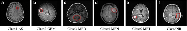
SROIs of tumors marked by radiologist using CBAC

Feature Extraction

Relevant set of 218 intensity and texture features are extracted from the SROIs. These features are: Laplacian of Gaussian (LoG), gray level co-occurrence matrix (GLCM), rotation invariant local binary patterns (RILBP), directional Gabor texture features (DGTF), intensity-based features (IBF), and rotation invariant circular Gabor features (RICGF). The features extracted are discussed below:

1. Laplacian of Gaussian (LoG): LoG filters at Gaussian widths of 0.25, 0.50, 1, and 2 are considered. These values are convoluted with the input image. Sixteen features are retrieved by calculating mean, standard deviation, skewness, and kurtosis for the LoG filter output in the SROI region.

2. Gray Level Co-occurrence Matrix (GLCM): Four textural features namely ‘Contrast’, ‘Homogeneity’, ‘Correlation’, and ‘Energy’ for four different offsets of GLCM are calculated, thereby contributing 16 features in the feature pool [7]. Assuming that is the GLCM of an image I(x, y) within the region I_B for an offset vector showing co-occurrence count of intensity pair i and j, the four features are defined as:

   • Contrast (C): Contrast of the image gives a measure of sudden change in intensity values in image which is calculated as given below:

     1.11
   • Correlation (S): It is a measure of correlation of a pixel to its neighbor within the selected region in the image.

     1.12
   • Homogeneity (H): It measures the closeness of the distribution of elements in the GLCM to the GLCM diagonal thereby showing uniformity in intensity values. The GLCM diagonal represents pixels having same intensity in their vicinity.

     1.13
   • Energy (E): It gives the sum of squared elements in the GLCM. More distributed is the GLCM, lower is its energy.

     1.14

3. Rotation Invariant Local Binary Patterns (RILBP): RILBP are used as they give measure of the irregularity and discontinuity within a SROI. Intensity pattern in the SROI is represented using histograms. Four intensity-statistical parameters namely: mean intensity, standard deviation, skewness, and kurtosis from the histogram of an image within the SROI are calculated. Nine filtered images are obtained by the use of range filter, standard deviation filter, and average filter with neighborhood of 7 × 7 on three LBP images of radii −1, 2, and 4 pixels. Four statistical features are calculated from these images and 36 features are added to the feature bank [17].

4. Intensity-Based Features (IBF): Intensity pattern in tumor region is modeled using histograms of target image and range filtered image. The histogram of an SROI image is represented byh(k). The brain tumor image intensity is represented as a function I (i, j) of two space variables I and j whereI (i, j) = 1, 2….N. The intensity I (i, j) can take k discrete values, where k is the total number of intensity levels in an image. Intensity-statistical parameters namely: mean intensity, standard deviation, skewness, and kurtosis from the histogram of an image within the tumor segment are calculated. The similar four parameters, for range filter output within the SROI contribute to four more features. Apart from these features, mean entropy of two image SROIs (original image and range filtered image) are also considered. Ten intensity features are added in the feature bank. These features are explained below:

   1.15

   • Mean (m): The mean (m) is defined as the sum of the intensity values of pixels divided by the number of pixels in the SROI of an image. Mean represents the first central moment and indicates the average level value of SROI where I (i, j) is the pixel intensity at position (i, j) and N represents the total number of pixels of SROI

     1.16
   • Standard Deviation (Std): The standard deviation is used to describe the spread of gray level around the mean.

     1.17
   • Skewness: The third central moment gives the skewness of the intensity distribution. It is the measure of symmetry and asymmetry of the gray level values around the mean.

     1.18
   • Kurtosis: The forth central moment gives kurtosis. It gives the measure of closeness of an intensity distribution to the normal Gaussian shape.

     1.19
   • Entropy: Entropy represents the amount of randomness in gray level intensity distribution of an image and corresponds to the grey levels which the individual pixels can adopt.

     1.20
5. Directional Gabor Texture Features (DGTF): Directional Gabor’s are used as they measure the heterogeneity in the SROI. Gabor filter is a Gaussian kernel function modulated by a sinusoidal plane wave. Therefore, it gives directional texture features at a specified Gaussian scale. Gabor kernel is defined as:

   1.21

   where

   In this equation, λ represents the wavelength of the sinusoidal factor, θ represents the orientation of the normal to the parallel stripes of a Gabor function, ψ is the phase offset, σ is the width of the Gaussian, and γ is the spatial aspect ratio, and specifies the ellipticity of the support of the Gabor function [18]. The value of γ is taken as 1.0, of is taken as ψ 0 and that of σ is taken as 0.56 λ. The θ (degrees) and λ (pixels) are varied for five different values viz. (2√2, 4, 4√2, 8, and 8√2) and (0°, 22.5°, 45°, 67.5°, and 90°) resulting in 25 different Gabor filter features. These features are then convoluted with the input image and the mean values of the output in the SROI are taken as 25 features in the feature bank. Mean, standard deviation, skewness, and kurtosis are the four statistical parameters extracted for each filter output in the marked SROI and are taken as 100 features in the feature bank.

6. Rotation Invariant Circular Gabor Features (RICGF): Gabor filter is a Gaussian kernel function modulated by a radially sinusoidal surface wave; therefore, it gives rotational invariant texture features which are given by:

   1.22

   where

   Here are coordinates of the center of Gaussian part in the filter, λ represents the wavelength of the sinusoidal factor, σ is Gaussian width, and ψ is the phase offset of the sinusoidal factor. Similar to directional Gabor filters, five values of λ viz. (2√2, 4, 4√2, 8, and 8√2) and two values of ψ, i.e., 0° and 90° are considered there by retrieving 10 features [19]. Mean, standard deviation, skewness, and kurtosis are the four statistical parameters which are extracted for each filter output in the marked SROI and are taken as 40 features in the feature bank.

The intensity and texture features summary is given in Table 1.

Table 1.

Summary of intensity and texture features

Feature category	Features	Number of features
LoG	Four statistical parameters for the LoG filter output in the SROI region are retrieved at σ = 0.25, 0.50, 1, and 2 thereby contributing 16 features in the feature pool. These parameters are: (1) mean intensity, (2) standard deviation, (3) Skewness, (4) Kurtosis
GLCM	Following GLCM features at 0°, 45°, 90°, and 135° are calculated: (1) contrast, (2) homogeneity, (3) correlation, (4) energy	4 × 4 = 16
RILBP	For LBP, LBP-range, and LBP standard deviation filter output for radii-1, 2, and 4 pixels are calculated. These features are: (1) mean intensity, (2) standard deviation, (3) Skewness, (4) Kurtosis	4 × 3 × 3 = 36
IBF	Following features for the histogram of an image and range filter output within the SROI are calculated: (1) mean intensity, (2) standard deviation, (3) Skewness, (4) Kurtosis, (5) entropy	5 + 5 = 10
DGTF	The λ for 2√2, 4, 4√2, 8, 8√2) and θ for 0°, 22.5°, 45°, 67.5°, and 90° are varied. Four statistical parameters are calculated for each filter output in the marked SROI and are taken as 100 features in the feature bank. These parameters are: (1) mean intensity, (2) standard deviation, (3) Skewness, (4) Kurtosis	25 × 4 = 100
RICGF	RICGFs are calculated at λ = 2√2, 4, 4√2, 8, 8√2) and two values of ψ, i.e., 0° and 90° four statistical parameters for each filter output in the marked SROI and are taken as 40 features in the feature bank. These features are: (1) mean intensity, (2) standard deviation, (3) Skewness, (4) Kurtosis	10 × 4 = 40
Total number of features:10 + 16 + 16 + 100 + 40 + 36 = 218

Feature selection using PCA

An optimal subset of features is extracted for producing best results. PCA is used for the reduction of dimensionality of the feature space in the proposed system. The complete dataset has been used to compute Eigen space for the features. Forty-nine Eigen features are selected. A linear transformation A_n^T is formed by PCA by transforming a random vector X ∊ R^m to a random vector of lower dimension of Y ∊ Rⁿ, m > n. The input random vectors X have zero mean and a covariance matrix ∑. The output (reduced dimensions) is obtained as Y = A_n^TX, where size of A_n^T is n × m. The whole training data set has been used for formation of covariance matrix. If the input data is initially of m dimensions, the covariance matrix is of size m × m. This covariance matrix is used to construct Eigen feature space and m Eigen vectors. The m dimensions are computed in decreasing order of their Eigen values. The transformation is obtained by retaining top n Eigen vector in terms of Eigen values thus forming transformation matrix A_n of size m × n. The values of m and n are significantly less than the number of samples where m is the number of total input features (m = 218) and n are the retained Eigen features (n = 49). The output feature vectors are obtained by projecting it to a new coordinate system and retaining the dimensions with maximum variations. The numbers of Eigen features retained are estimated by hit and trial method [20, 21].

Classification Module

In the artificial neural network, for solving regression problems, multi-layer perceptron supervised learning algorithm is used [20, 21]. As discussed in the previous section, the number of Eigen vectors retained for best classification capability is 49. Gradient descent back-propagation with momentum algorithm is used for estimating weights (training phase), momentum weight, and bias-based learning. The proposed network uses the momentum constant as 0.8 and learning rate of 0.02. Tenfold cross-validation is used during network training to avoid over-training and to improve generalization capability of the network. Hit and trial method is used to decide the network topology. It is observed that a reasonable tradeoff between accuracy and speed is achieved by the use of 18 neurons in the hidden layer.

Dataset and Software Implementation

The dataset used for the experimentation and the software implementation details are given in the next subsections.

Dataset

In the present study, 55 patients dataset constituting of −118 AS, 59 GBM, 97 MED, 88 MEN, 66 MET, and 428 NR are taken from 428 MR brain tumor slices and 856 SROIs are marked by the radiologists using CBAC. These images are collected from Department of Radiodiagnosis, Postgraduate Institute of Medical Education and Research (PGIMER), Chandigarh, India, over the time period of January 2010 to May 2011 and are acquired using MRI equipment (Siemens Verio, Erlangen, Germany, 3 Tesla MR Scanner). The number of SROIs for NRs is taken significantly larger than the malignant regions to well recognize highly varying anatomical regions. These tumors are graded and manually segmented by the radiologists based on their knowledge on visual image interpretation of brain tumors, clinical history of the patient, and disease confirmation by the biopsy/dynamic helical CT/MRI/pathological examinations. Percent of the dataset is used for training and 50 % is used for testing.

Software Implementation

Proposed method is implemented in MATLAB 8.0 and is tested on various brain tumor MR images of size 256 × 256. The experiments are performed on PC having Intel™ Core 2 Duo® 2.0 GHz processor with 3 GB RAM. The algorithm takes 25 min for training the samples. Testing time for both feature extraction as well classification of each SROI is 0.55 ms.

Experimental Set Up

Three set of experiments are performed to test the performance and robustness of PCA-ANN approach over ANN.

1. In the first experiment, six tumor classes are classified using ANN approach.

2. In the second experiment, random selection of data has been used. In random selection, SROIs from the same patient may appear in both training and testing simultaneously [22].

3. In the third experiment, to remove bias, the system is tested on a dataset which is completely unseen by the system. The basic data structure used for evaluation is confusion matrix. The performance of the proposed method is analyzed in terms of individual class accuracy and overall classification accuracy.

Given a confusion matrix as shown in Tables 2, 3, and 4 in context of brain tumor classification system the following parameters are defined:

1.23

1.24

where, TP(i) is correctly classified instances of class (i)

Table 2.

Confusion matrix for ANN approach

Class predicted	Ground truth class (assigned by radiologist)
	AS	GBM	MED	MEN	MET	NR
AS	42	8	1	4	0	8
GBM	10	20	1	0	0	10
MED	2	2	38	5	2	6
MEN	0	0	3	35	2	3
MET	5	0	2	5	30	5
NR	0	8	1	4	0	160
Individual class accuracy	71 %	66.67 %	84.4 %	71.4 %	88.2 %	83.3 %
Overall classification accuracy	77 %

Table 3.

Confusion matrix for PCA-ANN (random selection of SROIs)

Class predicted	Ground truth class (assigned by radiologist)
	AS	GBM	MED	MEN	MET	NR
AS	49	2	0	1	0	2
GBM	3	23	2	0	0	0
MED	0	0	34	0	0	6
MEN	0	0	0	39	0	3
MET	0	1	1	0	29	1
NR	2	0	3	3	1	181
Individual class accuracy (%)	90.74 %	88.46 %	85.00 %	90.70 %	96.67 %	93.78 %
Overall classification accuracy	91 %

Table 4.

Confusion matrix for PCA-ANN (SROIs are not common during training and testing)

Class predicted	Ground truth class (assigned by radiologist)
	AS	GBM	MED	MEN	MET	NR
AS	58	10	0	4	0	2
GBM	5	28	7	1	0	0
MED	0	4	14	0	4	6
MEN	4	1	1	54	4	3
MET	0	0	0	0	15	1
NR	0	0	0	0	0	160
Individual class accuracy (%)	86.15 %	65.1 %	63.36 %	91.5 %	65.21 %	93.3 %
Overall classification accuracy	85.23 %

Overall classification accuracy=

1.25

Results and Discussions

Experiments 1 and 2

In the first experiment, classification with ANN is performed. It is observed from Table 2 that overall classification accuracy of 77 % is obtained. Random sub-sampling has been used for testing the generalization ability of the proposed system. During random sampling, there may be a repetition of SROIs in testing data which may increase the accuracy of the proposed system. It is observed that the overall accuracy and individual class accuracy of PCA-ANN classifier is 91 % (Table 3). The proposed method has delivered a high accuracy for each class. The accuracy obtained for each class is: AS—90.74 %, GBM—88.46 %, MED—85.00 %, MEN—90.70 %, MET—96.67 %, and NR—93.78 %. Direct comparison with earlier methods has not been performed as dataset is not a standard one and has not been used by the existing methods. The accuracy obtained by earlier studies for class 2 lies in the range of 42 % whereas the proposed method has delivered an accuracy of 88.46 %. For class 4, i.e., MEN, PCA-ANN has delivered an accuracy of 90 %. It is observed from the previous studies that the accuracy obtained for class 5 lies is in the range of 87 to 95 % for class 5 (MET) whereas the proposed method has delivered an accuracy of 96.67 %. Class 1 (AS), class 3 (MED), and class 6 (NR) have not been considered in the earlier studies. It is also noticed from the experimentation that the selection of texture and intensity features by PCA and classification by ANN have given better classification results for all the classes.

Experiment 3

In the second experiment, data is partitioned in a manner such that the SROIs from the same patient are not common for training and testing sets. The proposed method has delivered an accuracy of 85.23 % (Table 4). It is observed that for class1 (AS), class 4 (MEN) and class 6 (NR), the accuracy obtained is 86.15 %, 91.5 % and 93.3 %. During testing, the number of SROIs for class 1, class 4 and class 6 are 67, 59 and 172 respectively. The number of data samples for these classes are higher in number during training and testing. Therefore, the accuracy obtained for class 6 is 93.3 %. Similarly, for other two classes, i.e., class 1 and class 4, the accuracy obtained lies in the range of 86 to 91 %. However, for other classes, i.e., class 2 (GBM), class 3 (MED), and for class 5 (MET), the accuracies lie in the range of 65 % as the number of SROIs for these three classes are very less 43, 22, and 23. Further, it is observed for class 2 (GBM) that this class is misclassified in class1 (AS; 10 samples out of 43 are misclassified in class 1). The possible reasons are GBMs are radiologically and pathologically similar to AS and secondly, lesser number of SROIs of GBMs during both training and testing time. It is noticed from the above discussion that the features extracted efficiently helps in discriminating the diseased tissues and the better results are obtained even on the unseen data. The generalization ability of this approach can be tested by analyzing larger datasets for each class. Larger samples taken during training will also further improve the performance of the proposed PCA-ANN approach.

For more crisp classification, dataset comprising of subclasses of a tumor, e.g., for astrocytoma class both low-grade and high-grade astrocytoma will be collected in the future and the proposed method will be tested on a wide diversified dataset. However, data collection may take a long span of time.

Conclusion

In this paper, CAD system is developed which includes segmentation, feature extraction, and multiclass classification of six classes of primary and secondary brain tumors along with normal region. These tumors may have similar characteristics in their intensity and texture pattern; however, these tumors differ in their location, size, and shape. CBAC is used for extracting tumor boundaries (SROIs). The performance of the system is evaluated using ANN and PCA-ANN approach on a dataset of 856 SROIs from 428 images. Two hundred eighteen texture and intensity features are extracted from the marked SROIs. PCA is use for reduction of dimensionality of the feature space and multiclass classification of brain tumors is performed using ANN. Three set of experiments are performed. In the first experiment, the SROIs selected are by random sampling process in which the SROIs of the same patient may get repeated during training and testing. From this experiment, it is observed that the high individual class accuracy and overall classification accuracy of 91 % is achieved (Table 3). The comparative analysis with ANN approach shows that PCA-ANN has increased the overall accuracy by 14 %. In the third experiment, the available patient data has been grouped into set of two data such that one set of SROIs is used for training and second set exclusive of SROIs of the patients in training are used for testing. This helps to remove the bias and test robustness and accuracy of the algorithm. It has been observed that even in this case higher overall accuracy (85.5 %) is achieved. Individual class accuracy nearing 65 % (Table 4) is observed of those classes which have lesser number of training and testing samples and in glioma classes such as AS and GBMs which have similar texture and intensity patterns and location. It is noticed that the proposed methodology has performed much better as compared to other state of art methods (even for AS and GBMs). However, inclusion of more number of patients per tumor class and addition of subclasses of astrocytomas—low-grade astrocytomas and high-grade astrocytomas will increase the generalization ability of the proposed approach. The performance of the proposed PCA-ANN approach can be further improved by extensive training. The developed methods for segmentation, feature extraction, and classification of brain tumors can be amalgamated to develop a CAD system. This system would be beneficial to radiologists for precise localization, diagnosis, and interpretation of brain tumors on MR images.

References

- 1.Caselles V. Geodesic active contours. Int J Comput Vision. 1997;22(3):61–79. doi: 10.1023/A:1007979827043. [DOI] [Google Scholar]
- 2.Clark MC, Hall LO, Goldgof DB, Velthuizen R, Murtagh FR, Silbiger MS. Automatic tumor segmentation using knowledge-based techniques. IEEE Trans Med Imaging. 1998;17(2):187–2011. doi: 10.1109/42.700731. [DOI] [PubMed] [Google Scholar]
- 3.Xu C, Prince JL. Snakes, shapes, and gradient vector flow. IEEE Trans Image Process. 1998;7(3):359–369. doi: 10.1109/83.661186. [DOI] [PubMed] [Google Scholar]
- 4.Lynn M, Lawerence OH, Demitry B, Goldgof RMF. Automatic segmentation of non-enhancing brain tumors. Artif Intell Med. 2001;21:43–63. doi: 10.1016/S0933-3657(00)00073-7. [DOI] [PubMed] [Google Scholar]
- 5.Dou W, Ruan S, Chen Y, Bloyet D, Constans J. A framework of fuzzy information fusion for the segmentation of brain tumor tissues on MR images. Image Vis Comput. 2007;25:164–171. doi: 10.1016/j.imavis.2006.01.025. [DOI] [Google Scholar]
- 6.Wang T, Cheng I, Basu A. Fluid vector flow and applications in brain tumor segmentation. IEEE Trans Biomed Eng. 2009;56(3):781–789. doi: 10.1109/TBME.2009.2012423. [DOI] [PubMed] [Google Scholar]
- 7.Haralick RM, Shanmugam K, Dinstein I. Textural features for image classification. IEEE Trans Systems Man Cybernet. 1973;3:610–621. doi: 10.1109/TSMC.1973.4309314. [DOI] [Google Scholar]
- 8.Selvaraj H, Thamarai Selvi S, Selvathi D, Gewali LB. Brain MRI slices classification using least squares support vector machine. J Intell Comput Med Sci. 2009;1:21–33. [Google Scholar]
- 9.Kharrat A, Gasm K. Hybrid approach for automatic classification of brain MRI using genetic algorithm and support vector machine. Leonardo Journal of Sciences. 2010;17:71–82. [Google Scholar]
- 10.Zacharaki EI, Wang S, Chawla S, Yoo DS, Wolf R, Melhem ER, Davatzikos C. Classification of brain tumor type and grade using MRI texture in a machine learning technique. Magn Reson Med. 2009;62:1609–1618. doi: 10.1002/mrm.22147. [DOI] [PMC free article] [PubMed] [Google Scholar]
- 11.Georgiardis P, Cavouras D, Kalatzis I, Daskalakis A, Kagadis GC, Malamas M, Nikifordis G, Solomou E. Improving brain tumor characterization on MRI by probabilistic neural networks on non-linear transformation of textural features. Comput Meth Prog Bio. 2008;89:24–32. doi: 10.1016/j.cmpb.2007.10.007. [DOI] [PubMed] [Google Scholar]
- 12.Georgiardis P, Cavouras D, Kalatzis I, Daskalakis A, Kagadis GC, Malamas M, Nikifordis G, Solomou E. Non-linear least square feature transformations for improving the performance of probabilistic neural networks in classifying human brain tumors on MRI. Lecture Notes on Computer Science. 2007;4707:239–247. doi: 10.1007/978-3-540-74484-9_21. [DOI] [Google Scholar]
- 13.El-Dahshan EA, Hosny T, Badeeh A, Salem M. Hybrid MRI techniques for brain image classification. Digital Signal Process. 2009;20:433–44. doi: 10.1016/j.dsp.2009.07.002. [DOI] [Google Scholar]
- 14.Specht DF. Probabilistic Neural Networks. 1990;3:109–118. doi: 10.1016/0893-6080(90)90049-Q. [DOI] [PubMed] [Google Scholar]
- 15.Ahmed NU, Rao R. Orthogonal transforms for digital signal processing. Heidelberg: Springer; 1975. [Google Scholar]
- 16.Sachdeva J, Kumar V, Gupta I, Khandelwal N, Ahuja CK. A novel content based brain tumor segmentation. Mag Reson Imaging. 2012;30(5):694–715. doi: 10.1016/j.mri.2012.01.006. [DOI] [PubMed] [Google Scholar]
- 17.Ojala T, Pietikäinen M, Mäenpää T. Multi resolution gray-scale and rotation invariant texture classification with local binary pattern. IEEE Trans Pattern Anal Machine Intell. 2002;24:971–998. doi: 10.1109/TPAMI.2002.1017623. [DOI] [Google Scholar]
- 18.Idrissa M, Acheroy M. Texture classification using Gabor filters. Pattern Recognition Lett. 2002;23:1095–1102. doi: 10.1016/S0167-8655(02)00056-9. [DOI] [Google Scholar]
- 19.Zhang J, Tan T, Ma L: Invariant texture segmentation via circular Gabor filters. In. Proc: Sixteenth International Conference on Pattern Recognition, Quebec City, Canada, 2: 901–904, 2002
- 20.Jain AK, Duin RPW, Jianchang M. Statistical pattern recognition. A review. IEEE Trans Pattern Anal Mach Intell. 2000;22:4–37. doi: 10.1109/34.824819. [DOI] [Google Scholar]
- 21.Duda RO, Hart PE, Stork DG. Pattern classification. New York: Wiley; 2001. [Google Scholar]
- 22.Kumar V, Sachdeva J, Gupta I, Khandelwal N, Ahuja C K: Classification of brain tumors using PCA-ANN. In Proceedings WICT, Mumbai, India, 1079–1083, 2011. doi:10.1109/WICT.2011.6141398